Methods and tools for synchronized visualization of evolving networks
Tam metin
Şekil
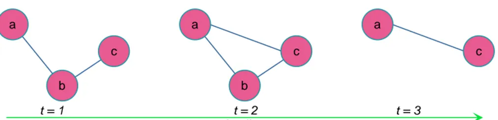
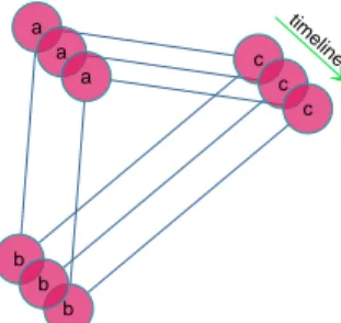
![Figure 3.1: A dynamic graph laid out with merged layout method [16]](https://thumb-eu.123doks.com/thumbv2/9libnet/5876709.121206/28.892.243.721.168.532/figure-dynamic-graph-laid-with-merged-layout-method.webp)
![Figure 3.2: A dynamic graph laid out with Foresighted layout algorithm [17]](https://thumb-eu.123doks.com/thumbv2/9libnet/5876709.121206/29.892.232.730.167.534/figure-dynamic-graph-laid-foresighted-layout-algorithm.webp)
![Figure 3.3: Screenshot of the user interface of GraphAEL [18]](https://thumb-eu.123doks.com/thumbv2/9libnet/5876709.121206/30.892.235.722.384.753/figure-screenshot-user-interface-graphael.webp)
![Figure 3.4: Screenshot of the user interface of Visone [19]](https://thumb-eu.123doks.com/thumbv2/9libnet/5876709.121206/31.892.235.727.165.536/figure-screenshot-user-interface-visone.webp)
![Figure 3.5: Screenshot of the user interface of Gevol [20]](https://thumb-eu.123doks.com/thumbv2/9libnet/5876709.121206/32.892.234.730.159.542/figure-screenshot-user-interface-gevol.webp)
Benzer Belgeler
McCaslin’in (1990), “Sınıfta Yaratıcı Drama” (Creative Drama in The Classroom) başlıklı çalışmasında, Meszaros’un (1999), “Eğitimde Yaratıcı Dramanın
Kilise ve devlet aynı kutsal otoritenin farklı yüzünü temsil etmektedir (s.. göre, çağdaş ulusal ve uluslararası siyasetin kaynağı ve arka planını oluşturduğunu
Örnek: Beceri Temelli
Son on ydda Türk Sinema sında büyük bir değişim olmuş, artan film sayısıyla birlikte renkli film tekniği yerleşmiş,. lâboratuvar işlemleri gelişmiş,
As far as the method and procedure of the present study is concerned, the present investigator conducted a critical, interpretative and evaluative scanning of the select original
For example; Codeine phosphate syrup, silkworm syrup, ephedrine hydrochloride syrup, paracetamol syrup, karbetapentan citrate syrup... General
The relationship between the location sequence characteristics of the hospital’s floor plan and wayfinding behavior performances was examined, and it was observed that there
When all data were merged, participants had an accuracy level that is significantly higher than 50% in detecting agreeableness (male and female), conscientiousness (male
