Original Research
Malignant-Lesion Segmentation Using 4D
Co-Occurrence Texture Analysis Applied to Dynamic
Contrast-Enhanced Magnetic Resonance Breast
Image Data
Brent J. Woods, MS,
1Bradley D. Clymer, PhD,
1,2* Tahsin Kurc, PhD,
3Johannes T. Heverhagen, MD, PhD,
4Robert Stevens, MD,
4Adem Orsdemir,
5Orhan Bulan,
5and Michael V. Knopp, MD, PhD
4Purpose: To investigate the use of four-dimensional (4D)
co-occurrence-based texture analysis to distinguish be-tween nonmalignant and malignant tissues in dynamic contrast-enhanced (DCE) MR images.
Materials and Methods: 4D texture analysis was
per-formed on DCE-MRI data sets of breast lesions. A model-free neural network-based classification system assigned each voxel a “nonmalignant” or “malignant” label based on the textural features. The classification results were com-pared via receiver operating characteristic (ROC) curve analysis with the manual lesion segmentation produced by two radiologists (observers 1 and 2).
Results: The mean sensitivity and specificity of the classifier
agreed with the mean observer 2 performance when com-pared with segmentations by observer 1 for a 95% confidence interval, using a two-sided t-test with␣ ⫽ 0.05. The results show that an area under the ROC curve (Az) of 0.99948, 0.99867, and 0.99957 can be achieved by comparing the
classifier vs. observer 1, classifier vs. union of both observ-ers, and classifier vs. intersection of both observobserv-ers, re-spectively.
Conclusion: This study shows that a neural network
clas-sifier based on 4D texture analysis inputs can achieve a performance comparable to that achieved by human ob-servers, and that further research in this area is warranted.
Key Words: texture analysis; DCE-MRI; neural network;
breast; cancer
J. Magn. Reson. Imaging 2007;25:495–501. © 2007 Wiley-Liss, Inc.
RADIOGRAPH MAMMOGRAPHY is currently regarded as the standard diagnostic tool for breast cancer detec-tion. Nevertheless, mammography has an associated 70% tumor detection rate (1), and only 10% to 33% of suspicious regions found in mammograms are deter-mined via biopsy to be cancerous (2). The sensitivity of mammography for breast cancer detection is reduced when dense fibroglandular breast tissue obscures the tumor. Since an estimated 30% of women are consid-ered to have dense breast tissue, mammography is not always considered reliable (1).
Dynamic contrast-enhanced magnetic resonance im-aging (DCE-MRI) is an alternative method for diagnos-ing breast cancer and can be used to monitor the effec-tiveness of cancer therapies on tumor growth. DCE-MRI can also be used to distinguish between tumor types and thus provide a “virtual biopsy.” Also, in con-trast to radiograph mammography, dense breast tissue does not interfere with the detection of tumors, and heterogeneous tumors are easily detectable. DCE-MRI has been shown to have a sensitivity of 85% to 100% and a specificity of 35% to 85% (3).
Although DCE-MRI has been shown to be effective in locating and classifying tumors, analysis of dynamic MRI data sets is time-consuming. Also, judgments as to the size, shape, and location of the tumor detected are influenced to some extent by intra- and interobserver variability. In this study, we propose a model-free, com-1
Department of Electrical and Computer Engineering, Ohio State Uni-versity, Columbus, Ohio, USA.
2
Department of Biomedical Engineering, Ohio State University, Colum-bus, Ohio, USA.
3
Department of Biomedical Informatics, Ohio State University, Colum-bus, Ohio, USA.
4
Department of Radiology, Ohio State University, Columbus, Ohio, USA.
5
Department of Electrical and Electronics Engineering, Bilkent Univer-sity, Ankara, Turkey.
Contract grant sponsor: National Institutes of Health (NIH), National Institute of Biomedical Imaging and Bioengineering (NIBIB) Biomedical Information Science and Technology Initiative (BISTI); Contract grant number: P20EB000591; Contract grant sponsor: National Science Foundation (NSF); Contract grant numbers: ACI-9619020 (UC subcon-tract 10152408); EIA-0121177; ACI-0203846; ACI-0130437; ANI-0330612; ACI-9982087; Contract grant sponsor: Lawrence Livermore National Laboratory; Contract grant number: B517095 (UC subcon-tract 10184497; Consubcon-tract grant sponsor: Ohio Board of Regents Bio-medical Research and Technology Transfer Consortium (BRTTC); Con-tract grant number: BRTT02-0003.
*Address reprint requests to: B.D.C, Department of Electrical and Com-puter Engineering, Ohio State University, 2015 Neil Ave., Columbus, OH 43210. E-mail: [email protected]
Received February 27, 2006; Accepted September 28, 2006. DOI 10.1002/jmri.20837
Published online 5 February 2007 in Wiley InterScience (www. interscience.wiley.com).
puter-aided diagnosis system for performing a voxel-by-voxel analysis of DCE-MRI data sets to detect ma-lignant tissues. Classification in this study was performed by 4D texture analysis along with a neural network.
Previous studies have applied texture analysis to medical imaging applications. Tourassi (4) discussed the role of texture analysis in the study of computer-aided diagnosis. Tourassi believes that texture analysis is a good means of extracting features from medical image data sets because radiologists rely on textures to make diagnostic decisions. Lerski et al (5) described how texture analysis can be used to classify tissues, and showed that texture analysis can be used to seg-ment brain regions from MR images. Gibbs and Turn-bull (6) applied co-occurrence-based texture analysis to postcontrast MR breast images. They were able to show that benign and malignant lesions differ in terms of the spatial variations in voxel intensities.
Tzacheva et al (7) proposed a method of detecting malignant tissues given an input-static, postcontrast, T1-weighted image slice. Static region descriptors are calculated, and a neural network classifier is then used to classify each region as malignant or nonmalignant. The classification system produced a reported 90% to 100% sensitivity and 91% to 100% specificity. Although good performance was reported, this system uses re-gion-based analysis rather than voxel-by-voxel analy-sis. Also, this system does not take advantage of the voxel signal intensity changes over the entire DCE-MRI time sequence.
Lucht et al (8,9) tested a model-free voxel-by-voxel tissue classification system. The system takes as input a 28-measurement point normalized time vs. signal in-tensity curve for a voxel. A neural network is used to assign one of three labels (carcinoma, benign lesion, or parenchyma) to the voxel. Discrimination between le-sion voxels (both malignant and benign) and paren-chyma voxels produced a performance of 96% sensitiv-ity and 90% specificity. Discrimination between malignant lesion voxels and benign lesion voxels pro-duced a performance of 84% sensitivity and 81% spec-ificity.
A recent paper by Twellmann et al (10) described a classifier that combines both supervised and unsuper-vised techniques, and takes as input the signal inten-sity vs. time information for a voxel. The classification results were compared with the results of manual le-sion segmentation done using the model-based three-time-point technique (11). A performance analysis showed that the classifier produced a receiver operating characteristics (ROC) curve with an area under the curve (Az) of 0.986 for malignant tissues. Although they reported good results, Twellmann et al (10) suggested that the addition of textural features may enhance the discriminative power of their classifier.
The work presented in this study uses four-dimen-sional (4D) co-occurrence-based texture analysis to dis-tinguish between nonmalignant and malignant tissues from DCE-MR images. With the use of texture analysis, statistical information regarding the change of voxel intensities over time is gathered. The textural features are the input to a model-free neural network-based
classification system that assigns each voxel a “nonma-lignant” or “ma“nonma-lignant” label on a voxel-by-voxel basis. The system’s classification results are compared via ROC analysis with the manual lesion segmentation per-formed by a radiologist using the two-compartment model. We recognize that interobserver variations occur during manual segmentation. Therefore, a second radi-ologist manually marked the lesion as well. We compare the lesion marked by the second radiologist with the lesion marked by the first radiologist using the first radiologist as the ground truth (gold standard). Using ROC analysis and comparing segmentations, we show that the neural network classifier achieves a perfor-mance comparable to that achieved by the second ra-diologist.
MATERIALS AND METHODS MRI Acquisition
In this study we retrospectively examined DCE-MRI data from four women with a total of four malignant invasive ductal carcinoma (IDC) lesions, and two women with a total of four benign (BEN) fibrocystic lesions. We performed all DCE-MRI data set acquisi-tions and analyses following the approved practices of our internal review board regarding the use of human subjects and data. The diagnosis of each lesion was histologically confirmed by biopsy of the lesion. All MRI acquisitions were performed on a 1.5 Tesla MR system (Magnetom Vision; Siemens, Erlangen, Germany). A dy-namic T1-weighted gradient-echo sequence (TR⫽ 8.1 msec, TE⫽ 4.0 msec, flip angle ⫽ 20°) was performed, and a total of 64 coronal slices (each slice consisting of 256 ⫻ 256 pixels) were obtained. Each slice had an effective slice thickness of 2.5 mm and a field of view (FOV) of 320⫻ 320 mm2. The dynamic image sequence
was acquired under the following protocol: Paramag-netic MultiHance Gd-BOPTA (Bracco Diagnostics Inc., Milan, Italy) was used as the contrast agent. A contrast agent dose of 0.2 mL/kg bodyweight was used, and the constant bolus injection duration was seven seconds. A total of six volumes per data set were acquired at six different time points. The first volume set was acquired to establish baseline intensity, and another five volume scans were taken 120 seconds apart to monitor the uptake and elimination of the contrast agent.
As is typically done in breast MRI, each patient lay prone in the breast coil with her arms extended above her head. The breasts were supported in order to re-duce motion caused by breathing, cardiac, and other movements. However, some motion due to voluntary, breathing, cardiac, and breast-settling motions is likely to occur in such examinations. Although algorithms (12,13) exist to correct for motion, no registration algo-rithms were used in this study.
Manual Segmentation by Radiologists
In order to train the neural network-based classifier and test the efficacy of the classifier, two trained radi-ologists (observers 1 and 2) performed manual segmen-tation of the lesions. The segmensegmen-tations performed by observer 1 served as the gold standard, and those made
by observer 2 were used to establish and quantify in-terobserver variability. Neither radiologist had knowl-edge of the segmentations made by the other observer. Manual segmentation was performed using a phar-macokinetic two-compartment-based analysis tool (14,15) implemented in IDL (Interactive Data Language, Boulder, CO, USA). The estimated pharmacokinetic pa-rameters A and kepwere color-coded and superimposed on the precontrast MR image. The radiologists then manually outlined the lesions using a computer mouse. Each lesion was assigned an “IDC” or “BEN” label de-pending on whether the lesion was malignant or be-nign. We recognize that some lesions are inhomoge-neous and have both malignant and benign characteristics (16,17); however, each lesion was as-signed only one label by the radiologist.
Texture Analysis
The goal of texture analysis is to quantify the depen-dencies between neighboring pixels and patterns of variations in image brightness within a region of inter-est (ROI) (4,18). In texture analysis, one can obtain useful information by examining local variations in im-age brightness. Haralick texture analysis (19) is a form of statistical texture analysis that utilizes co-occur-rence matrices to relay the joint statistics of neighbor-ing spatial or temporal voxels. A second-order joint con-ditional histogram (also called a co-occurrence matrix) is computed given a specific distance between pixels and a specific direction. The two random variables are the gray level of one pixel (g1) and the gray level of its
neighboring pixel (g2), and the neighborhood between
two pixels is defined by a user-specified distance and direction. Once a co-occurrence matrix is computed, statistical parameters can be calculated from the ma-trix. The 14 textural features described by Haralick et al (19) provide a wide range of parameters that can be used in medical imaging analysis.
In medical images, many localized texture changes denoting tumors, vessels, and different tissues may ex-ist. Thus, it is often necessary to apply a series of tex-ture calculations with each calculation performed on a localized region. 4D texture analysis begins with the selection of a 4D scanning window. The voxels within this window are used to generate a co-occurrence ma-trix, and the matrix is used to generate the Haralick textural features. For example, a 5⫻ 5 ⫻ 3 ⫻ 2 (x, y, z,
t) scanning window would cover a 5⫻ 5 in-slice region
spread across three coronal slices and two time sam-ples. The scanning window is moved throughout the 4D DCE-MRI data set, and textures are computed at each movement of the window. The window is first moved along the x-dimension, which is from the left to the right of the patient. The window is then moved along the
y-dimension (inferior to superior) and then along the z-dimension (posterior to anterior). Finally, the window
is moved in the t-dimension from precontrast to the final acquisition in the temporal sequence. Although texture analysis is a computationally intensive process, it can be performed quickly and efficiently with the use of parallel computing (20).
Features Used
Given an input DCE-MRI data set, features may be extracted that depend on the Haralick feature parame-ter, scanning window size, and voxel neighbor direction and distance used for co-occurrence matrix calcula-tions. First, we always use the direction (0x, 0y, 0z, 1t) and a distance value of one to generate the co-occur-rence matrices. Using the (0, 0, 0, 1) direction allows us to generate co-occurrence matrices based on variations in image brightness that occur between the same voxel location at different time samples. This direction is use-ful for classification because our DCE-MRI data sets are assumed to be only time-varying. This assumption is not always accurate, however, since patient motion can create spatial voxel intensity variations in addition to the temporal variations.
Next we use our knowledge of the time vs. voxel in-tensity curves to decide which Haralick textures, scan-ning windows, and range of time segments to use. A 5⫻ 5 ⫻ 1 ⫻ 2 (x, y, z, t) scanning window is used to calculate the Haralick contrast parameter from consec-utive time samples. For malignant tissues, the contrast parameter at time windows starting at t1and t2
corre-sponds to contrast agent uptake, and the contrast pa-rameter starting at t3, t4, and t5corresponds to contrast
agent elimination. For malignant tissues, these time windows should have different contrast levels com-pared to nonmalignant tissues. A 5⫻ 5 ⫻ 1 ⫻ 3 scan-ning window is used for the difference variance and inverse different moment parameters to gather statis-tics for contrast agent uptake at the time window start-ing at t1. A 3⫻ 3 ⫻ 1 ⫻ 6 scanning window is used for
the sum of squares (SOS) and difference entropy pa-rameters. This scanning window accounts for all tem-poral variations within the scanning window.
In our classification system, we vary the scanning window size depending on the Haralick parameter used, which is typically not done in other tissue classi-fication applications. However, this allows us to focus the scanning window on a chunk of data that is most beneficial for classification purposes while maintaining a scanning window size that does not violate the law of large numbers when producing a co-occurrence matrix. The result is a statistically valid co-occurrence matrix produced by a region of data in which we are specifically interested. This feature-selection process yields nine total features that are inputs to the neural network used to detect malignant tissues.
Training and Classification
The classifier developed in this project is a neural net-work-based classifier implemented in Matlab (Math-Works Inc., Natick, MA, USA). A four-layer feed-forward back-propagation neural network was created using the Matlab Neural Network Toolbox. The first three lay-ers each contained nine nodes, and the last layer con-tained a single node. The network used pure linear transfer functions and was batch-trained using the Levenberg-Marquardt algorithm.
The training set consisted of a collection of malignant (IDC) and nonmalignant (parenchymal and BEN) vox-els. The IDC training voxels were randomly chosen from
two IDC lesions as segmented by observer 1. The first lesion had a higher than average level of enhancement as compared to the baseline intensity, and the second lesion had a lower than average level of enhancement. Therefore, voxels from these two lesions offer a wide variation of texture parameters corresponding to the “malignant” label. The “nonmalignant” training voxels were chosen from a single BEN lesion as segmented by observer 1. Approximately 10% of the voxels within the lesions were used for training. Additional nonmalignant training voxels were taken randomly from the paren-chymal breast tissue that was not marked as lesion by observer 1. An approximately equal number of malig-nant and nonmaligmalig-nant voxels were used for training. Once trained, the classifier can be presented with a pattern of textures for a given voxel. The voxel is then assigned either a “malignant” or “nonmalignant” label.
Evaluation of Results
After the neural network is trained and a data set is tested, it is useful to present the results in a fashion that allows for easy analysis. One approach is to create a series of output images that depict how the neural network-classified voxels compare with the radiologist-marked images. Color-coded output images provide the user with a quick visual means of determining the per-formance of the neural network. However, it is often beneficial to see how voxel classification relates to an-atomical structures. Thus, when we present classifier output image results, we superimpose the classifier re-sults on the anatomical images taken from the DCE-MRI baseline scan. For our output images we employ the following color scheme: yellow⫽ true positive (TP), black/grayscale⫽ true negative (TN), green ⫽ false pos-itive (FP), and red⫽ false negative (FN).
In addition to a visual analysis, a statistical analysis can also be used to quantify classifier performance. The TP fraction (TPF) and FP fraction (FPF) are two condi-tional probabilities that can be calculated for analysis purposes (21). We define the TPF as the rate at which the neural network flagged the voxel as being tumor tissue, when the radiologist marked the voxel as being tumor tissue (which is similar to sensitivity). Similarly, we define the FPF (or false-alarm rate) as the rate at which the neural network flagged the voxel as being tumor tissue, when the radiologist did not mark the
voxel as being tumor tissue (which is similar to the inverse of specificity).
We sample the output at various thresholds between 0 and 100. At each threshold, we produce a collection of output images and statistics that are useful for choos-ing a good threshold and evaluatchoos-ing the performance of the neural network training. The TPF (sensitivity) and the FPF (1-specificity) can be plotted. The resulting plot is an ROC curve. An optimal classifier maximizes the area under the ROC curve, and therefore the area under the curve (Az) is a measure of classifier performance. We note that voxels used for training are excluded from statistical analysis because they may bias the results.
RESULTS
Table 1 shows the size of each IDC lesion as indicated by manual segmentation of the lesion by two separate radiologists. Using observer 1 as the gold standard, we determined the percent difference between the two le-sion volumes reported by the radiologists. On a study-by-study basis, we found that the percent difference varied from 6.74% to 34.56% depending on the size, irregularity in shape, and overall enhancement of the tumor. We note that the largest percent difference be-tween the two observers occurred in the smallest lesion, where small variations led to large percent differences. We also found that there was only a 1.56% difference between the average volumes. Thus, on average we can-not say that one particular radiologist was more con-servative than the other in marking the lesions.
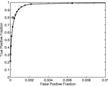
After we trained the neural network as described above, we tested the classifier using voxels that were not used for training. Figure 1 shows the ROC curve produced by comparing the neural network output with the manual segmentation by observer 1 for the six stud-ies. Each data point (x) on the curve corresponds to a Table 1
Volume of Each IDC Tumor as Reported by Manual Lesion Segmentations by Two Separate Radiologists*
Lesion number Lesion volume (observer #1) (cm3) Lesion volume (observer #2) (cm3) Percent difference (%) IDC1 27.39 30.94 ⫹12.96 IDC2 24.88 22.27 –10.49 IDC3 1.36 0.89 –34.56 IDC4 7.71 8.23 ⫹6.74 Average 15.34 15.58 ⫹1.56
*The percent difference in volume is shown for each lesion using observer #1 as the gold standard. The average lesion volume was computed for each observer and the percent difference was found.
Figure 1. The ROC performance curve produced by
compar-ing the neural network output with the manual segmentation by observer 1. The circle (E) denotes the performance of ob-server 2 as compared to the gold standard (obob-server 1). Sta-tistics were gathered by testing all IDC, BEN, and normal voxels that were not used for training.
sampling of the neural network output at a certain threshold. The data point denoted by a circle (E) indi-cates the average FPF vs. TPF derived by comparing the results of observer 2 with the gold standard of ob-server 1.
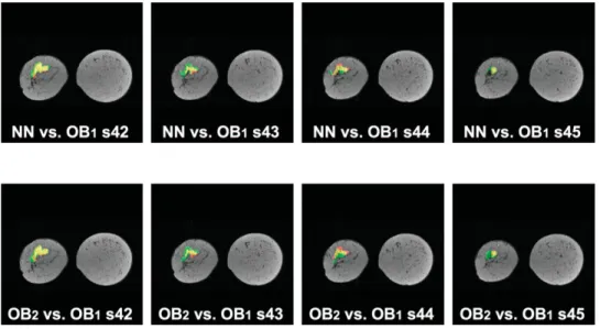
The vast majority of slices had good agreement be-tween the neural network classifier and observer 1, and agreement between observers 1 and 2. In Figs. 2– 4 we note some of the key differences. Figure 2 (top) provides a visualization of the performance of the neural network as compared to lesion segmentation by observer 1 for four selected slices of the IDC1study. Figure 2 (bottom)
illustrates the segmentation performance of observer 2 compared to segmentation by observer 1 for the same lesion. Figure 3 illustrates a similar comparison for selected slices of the IDC2study. Figure 4 shows neural
network classification errors (FPs) that arose due to incorrect classification of benign lesions, blood vessels, and patient motion.
In practice, the ground-truth segmentations used for training the classifier may be derived from a combina-tion (i.e., union or interseccombina-tion) of segmentacombina-tions pro-vided by several radiologists. Figure 5 shows the
per-formance of the classifier when it was trained and tested using the union of the segmentations provided by the two radiologists as the ground truth, and using the intersection of the segmentations as the ground truth. In Table 2 we list the area under the ROC curve
Azfor the neural network vs. segmentations by observer
1, neural network vs. union of segmentations by ob-servers 1 and 2, and neural network vs. intersection of segmentations by observers 1 and 2.
DISCUSSION
The results of this study show that texture analysis can be used to quantify variations in voxel intensities over time, and can be used along with a neural network to segment malignant lesions from DCE-MRI data sets. The system allows for adjustable thresholds, which gives the radiologist the option of choosing which sen-sitivity and specificity range to use for evaluation. For example, a threshold of 45 produces a sensitivity of 78.77% and a specificity of 99.96%, and a threshold of 25 produces a sensitivity of 96.22% and a specificity of 99.85%. We show in Fig. 1 that a threshold of 45 yields
Figure 2. Performance results
superimposed on anatomy for the IDC1 study. Yellow ⫽ TP,
black/grayscale⫽ TN, green ⫽ FP, red⫽ FN. Top: Neural net-work classification results us-ing a threshold of 45 compared with segmentation by observer 1. Bottom: Segmentation by observer 2 compared with seg-mentation by observer 1.
Figure 3. Performance results
superimposed on anatomy for the IDC2 study. Yellow ⫽ TP,
black/grayscale⫽ TN, green ⫽ FP, red⫽ FN. Top: Neural net-work classification results us-ing a threshold of 45 compared with segmentation by observer 1. Bottom: Segmentation by observer 2 compared with seg-mentation by observer 1.
a performance closest to that achieved by the human experts. Statistically, the mean TPF and FPF at a threshold of 45 agree with the mean observer 2 perfor-mance for a 95% confidence interval using a two-sided t-test with significance level␣ ⫽ 0.05.
The majority of FPs and FNs occur in the vicinity of the lesion, especially around the border of the lesion. During manual segmentation, the radiologist must out-line the lesion by hand using a computer mouse, which will likely cause some errors in the gold-standard data set. Also, voxels along the border of the tumor likely suffer from partial-volume effects because the tumor is spreading to neighboring tissues, which causes some (albeit not significant) enhancement. Such effects lead to reported misclassifications along the lesion’s border, and may also contribute to intra- and interobserver variations. For these reasons, we compare the manual segmentation by a second radiologist with the gold-standard segmentation. In Fig. 2 (top) we notice that a significant amount of FPs occur in slice 41. However, in Fig. 2 (bottom) we notice that segmentation by observer 2 also had FPs in the same region of slice 41. Thus, the classifier agrees more with observer 2 than with ob-server 1. Similar results are clearly shown in slice 26 of Fig. 3.
FPs also occur away from the malignant lesions and are caused by enhancing tissues and patient motion. Certain tissues, such as benign fibrocystic lesions and
blood vessels, experience contrast enhancement. Nor-mally, the neural network classifies benign lesions and blood vessels as nonmalignant tissue; however, in some cases benign lesions and blood vessels are misclassified as malignant, as shown in Fig. 4 (left) and (middle). Patient motion can also cause misclassifications, espe-cially around the edge of the breast, as shown in Fig. 4 (right). Future studies will examine whether texture analysis can be used to detect patient motion and hence alert the radiologist to possible data corruption. Texture analysis may also allow for motion correction since the co-occurrence matrix used to derive the tex-tures is direction-sensitive through a 4D hyperspace.
From Fig. 5 and Table 2 we notice that segmentations produced by the neural network have very good agree-ment with the segagree-mentations produced by taking the intersection of the segmentations by observers 1 and 2. That is, the neural network, observer 1, and observer 2 reach a consensus on which regions should be marked as malignant. When we compare the segmentations made by the neural network with those produced by taking the union of the segmentations by observers 1 and 2, there is less agreement. This is because we are now considering more of the border regions of the tu-mor, where more variations in segmentations are likely to occur. We note that the areas under all three ROC curves shown in Table 2 are an improvement over the average ROC curve area presented by Twellmann et al (10).
In conclusion, texture analysis along with a neural network classifier has the potential to aid radiologists in the detection and marking of malignant lesions. Our goal is not to replace the radiologist in malignant-lesion detection, but rather to offer the radiologist a tool for detecting tumors faster and more consistently. This study shows that manual segmentation methods suffer from interobserver variations, and the classifier pre-sented in this paper can be used to draw the radiolo-gist’s attention to questionable regions. The classifier achieves a performance comparable to that achieved by
Figure 4. Neural network FP
errors due to incorrect classifi-cation of (left) benign fibrocys-tic lesion, (middle) blood ves-sel, and (right) patient motion.
Table 2
Area Under the ROC Performance Curve Is Measured According to the Segmentations Used for Training and Testing of the IDC, BEN, and Normal Voxels
Gold standard segmentations Area under ROC curve
Observer #1 0.99948
Union of observers #1 and #2 0.99867 Intersection of observers #1 and #2 0.99957
Figure 5. The ROC performance curve produced by
compar-ing the neural network output with manual segmentation by observers 1 and 2.
human manual analysis using the pharmacokinetic two-compartment model. Although some misclassifica-tions can occur in areas away from the tumor, these FPs account for only a small fraction of the FPs. The majority of FPs occur near the border of the lesion. It is important to note that the classifier never failed to iden-tify the malignant lesions in our test cases. The results presented in this paper suggest that further study us-ing 4D co-occurrence-based texture analysis would be worthwhile, and we plan to extend our research to in-clude more studies and analyses by additional radiolo-gists.
REFERENCES
1. Kawashima H, Matsui O, Suzuki M, et al. Breast cancer in dense breast: detection with contrast-enhanced dynamic MR imaging. J Magn Reson Imaging 2000;11:233–243.
2. Feig SA. Breast masses: mammographic and sonographic evalua-tion. Radiol Clin N Am 1992;30:67–92.
3. Rankin SC. MRI of the breast. Br J Radiol 2000;73:806 – 818. 4. Tourassi GD. Journey toward computer-aided diagnosis: role of
image texture analysis. Radiology 1999;213:317–320.
5. Lerski RA, Straughan K, Schad LR, Boyce D, Bluml S, Zuna I. MR image texture analysis—an approach to tissue characterization. Magn Reson Imaging 1993;11:873– 887.
6. Gibbs P, Turnbull LW. Textural analysis of contrast-enhanced MR images of the breast. Magn Reson Med 2003;50:92–98.
7. Tzacheva AA, Najarian K, Brockway J. Breast cancer detection in gadolinium-enhanced MR images by static region descriptors and neural networks. J Magn Reson Imaging 2003;17:337–342. 8. Lucht R, Delorme S, Brix G. Neural network-based segmentation of
dynamic MR mammographic images. Magn Reson Imaging 2002; 20:147–154.
9. Lucht R, Knopp M, Brix G. Classification of signal-time curves from dynamic MR mammography by Neural Networks. Magn Reson Im-aging 2001;19:51–57.
10. Twellmann T, Lichte O, Nattkemper T. An adaptive tissue charac-terization network for model-free visualization of dynamic contrast-enhanced magnetic resonance image data. IEEE Trans Med Imag-ing 2005;24:1256 –1266.
11. Weinstein D, Strano S, Cohen P, Fields S, Gomori JM, Degani H. Breast fibroadenoma: mapping of pathophysiologic features with three-time-point, contrast-enhanced MR imaging pilot study. Ra-diology 1999;210:233–240.
12. Lucht R, Knopp M, Brix G. Elastic matching of dynamic MR mam-mographic images. Magn Reson Med 2000;43:9 –16.
13. Kerwin WS, Cai J, Yuan C. Noise and motion correction in dynamic contrast-enhanced MRI for analysis of atherosclerotic lesions. Magn Reson Med 2002;47:1211–1217.
14. Brix G, Semmler W, Port R, Schad L, Layer G, Lorenz W. Pharma-cokinetic parameters in CNS Gd-DTPA enhanced MR imaging. J Comput Assist Tomogr 1991;15:621– 627.
15. Taylor JS, Tofts PS, Phil D, Port R, Evelhoch J, Knopp M. MR imaging of tumor microcirculation: promise for the new millenium. J Magn Reson Imaging 1999;10:903–907.
16. Kuhl CK, Mielcareck P, Klaschik S, et al. Dynamic Breast MR imaging: are signal intensity time course data useful for differential diagnosis of enhancing lesions? Radiology 1999;211:101–110. 17. Collins D, Padhani A. Dynamic magnetic resonance imaging of
tumor perfusion: approaches and biomedical challenges. IEEE Eng Med Biol 2004:65– 83.
18. Conners RW, Harlow CA. A theoretical comparison of texture algo-rithms. IEEE Trans Patt Anal Machine Intell 1980;PAMI-2:204 –222. 19. Haralick RM, Shanmugam K, Dinstein I. Textural features for image
classification. IEEE Trans Syst Man Cybernet 1973;3:610 – 621. 20. Woods BJ, Clymer B, Saltz J, Kurc T. A parallel implementation of
4Dimensional Haralick texture analysis for disk-resident image datasets. In: Proceedings of the ACM/IEEE SC2004 Conference, Pittsburgh, PA, USA, 2004.
21. Rosner B. Fundamentals of biostatistics. 5th ed. Duxbury: Thom-son Learning; 2000.