Γ Η i:.... - .
H6' ,
Sf-Oé-5
•18
С 58
1933
С·!
L ѴТ' ' ''Ѵ - Ni -, ' ''· i f и / ·'* ; -^ :r¡v .;AN INVESTIGATION OF ANOMALIES
AT ISTANBUL SECURITIES EXCHANGE:
SIZE AND E/P EFFECTS
A THESIS
Submitted to the Faculty of Management
and the Graduate School of Business Administration
of Bilkent University
in Partial Fulfillment of the Requirements
For the Degree of
Master of Business Administration
By
HAKAN CiVELEKOÖLU
July, 1993
H G
5
^
-
Ъ
T z
c 'Эc-l
ß022925
I certify that I have read this thesis and in my opinion it is fully adequate, in scope and quality, as a thesis for the degree of the Master of Business Administration.
Assoc. Prof. Kür$at Aydogan
I certify that I have read this thesis and in my opinion it is fully adequate, in scope and quality, as a thesis for the degree of the Master of Business Administration.
Assist. Prof. Gülnur Muradoğlu Şengül
I certify that I have read this thesis and in my opinion it is fully adequate, in scope and quality, as a thesis for the degree of the Master of Business Administration.
Assist. Prof. Haluk Akdoğan
Approved for the Institute of Management Sciences
\ / V , .
ABSTRACT
AN INVESTIGATION OF ANOMALIES AT ISTANBUL SECURITIES EXCHANGE:
SIZE AND E/P EFFECTS
HAKAN CiVELEKOGLU M.B.A. in Management
Supervisor: Assoc. Prof. Kur?at Aydogan July 1993, 50 pages
This study investigates the presence of 'size- effect' and 'E/P effect' at Istanbul Securities Exchange for the period January 1990-December 1992.
24 months of monthly return data prior to test year are used to estimate the market risk of each stock. Each ear, portfolios are formed according to the previous year's E/P ratio and market value and than the average monthly returns of the current year are compared. In addition, to determine which of the variables significantly explain the average return of stocks, cross-sectional regression approach of Fama-MacBeth (1973) is applied.
The results reveal that there exists a weak 'E/P effect' in the years 1991 and 1992. However, a significant 'size effect' is not encountered at ISE as opposed to the case in developed capital markets.
K e y w o r d s :
anomaly
ÖZET
İSTANBUL MENKUL KIYMETLER BORSASINDA b i r ANOMALİ ARAŞTIRMASI:
FİRMA BÜYÜKLÜĞÜ VE K/F ETKİSİ
HAKAN CİVELEKOĞLU
Yüksek Lisans Tezi, İşletme Enstitüsü Tez Yöneticisi: Doç. Dr. Kürşat Aydoğan
Temmuz 1993, 50 sayfa
Bu çalışma İstanbul Menkul Kıymetler Borsasında firma büyüklüğü etkisi ve kazanç/fiyat (K/F) oranı etkisi olup olmadığını Ocak 1990 - Aralık 1992 döneminde
araştırmaktadır. ,
Ele alınan dönemde her sene için, o seneden önceki 24 aylık getiri miktarları çalışmaya dahil edilen her
hisse senedinin pazar riskini hesaplamak için
kullanılmıştır. Her sene, hisse senetleri bir önceki senenin firma büyüklüğü ve K/F oranı değerlerine göre sıralanarak pörtföyler oluşturulmuş ve portföylerin o seneki aylık getirileri mukayese edilmiştir. Bundan başka,
hangi değişkenlerin hisse senedi getirilerini
istatistiksel olarak açıkladığını tespit etmek için Fama- MacBeth'in kesit regresyonu metodu tatbik edilmiştir.
Sonuçlar 1991 ve 1992 senelerinde zayıf bir K/F oranı etkisi tespit etmiştir. Bununla beraber, gelişmiş sermaye piyasalarında rastlanan firma büyüklüğü etkisi IMKB de rastlanmamıştır.
Anahtar Kelimeler: Pazar etkinliği, piyasa değeri etkisi, kazanç/fiyat (K/F) oranı etkisi, anomali
ACKNOWLEDGEMENTS
I wish to express my gratitude to Associate Professor Kürşat Aydoğan for his invaluable supervision during the preparation of this thesis. I also wish to express my thanks to Assistant Professor Gülnur Muradoğlu Şengül and Assistant Professor Halûk Akdoğan for their helpful comments.
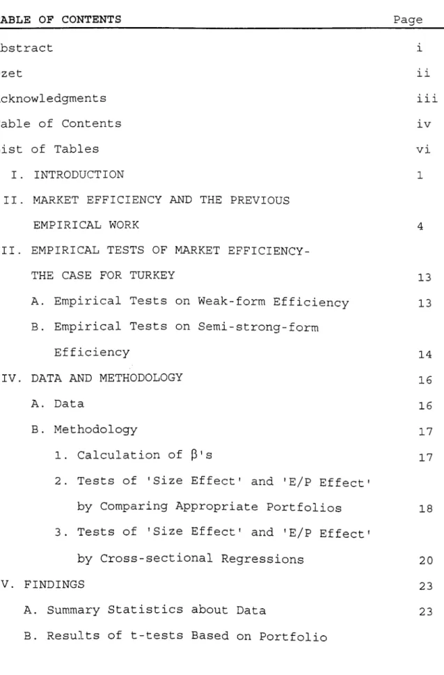
TABLE OF CONTENTS
Page Abstract Özet Acknowledgments Table of Contents List of Tables I . INTRODUCTIONII. MARKET EFFICIENCY AND THE PREVIOUS EMPIRICAL WORK
III. EMPIRICAL TESTS OF MARKET EFFICIENCY- THE CASE FOR TURKEY
A. Empirical Tests on Weak-form Efficiency B. Empirical Tests on Semi-strong-form
Efficiency
IV. DATA AND METHODOLOGY A. Data
B . Methodology
1. Calculation of (3's
2. Tests of 'Size Effect' and 'E/P Effect by Comparing Appropriate Portfolios 3. Tests of 'Size Effect' and 'E/P Effect
by Cross-sectional Regressions V. FINDINGS
A. Summary Statistics about Data
B. Results of t-tests Based on Portfolio
11 111 I V V I 1 13 13 14 16 16 17 17 18 20 23 23 IV
Formation Method
C. Results of t-tests Based on Cross-sectional Regressions Method
VI. CONCLUSIONS
VII. LIST OF REFERENCES APPENDICES 25 33 36 39 44
LIST OF TABLES
Table lA. Summary Statistics of E/P Value Quintiles, 1990.
and Market
26 Table IB. Summary Statistics of E/P
Value Quintiles, 1990.
and Market
27 Table 1C. Summary Statistics of E/P
Value Quintiles, 1990.
and Market
28 Table 2A. Comparison of High and Low
E/P Ratio Portfolios
Market
Value-30 Table 2B . Comparison of High and Low
E/P Ratio Portfolios
Market
Value-31 Table 2C. Comparison of High and Low
E/P Ratio Portfolios
Market
Value-32 Table 3 . Results of Cross-sectional Regressions 34
I . INTRODUCTION
According to market efficiency hypothesis, security prices reflect all relevant information in an efficient market. A vast amount of research has been conducted on market efficiency tests in capital markets. Research on market efficiency has been divided into three categories; weak-form tests, semi-strong- form tests and strong-form tests. Instead of weak-form tests which are traditionally concerned with only the forecast power of past returns, this category has been recently covering the more general area of tests of return predictability (Fama (1991)).
Due to joint hypothesis problem, market efficiency per se is not testable. It must be tested jointly with some model of equilibrium, an asset pricing model. This statement suggest that we can only test whether information is properly reflected in the context of the equilibrium pricing model (Fama (1970)). Since market efficiency and equilibrium- pricing issues are inseparable, the concept of predictability also considers the cross-sectional predictability of returns, that is, tests of asset pricing models and the anomalies discovered in the tests.
Among the other asset-pricing models, model of Sharpe (1964) , Lintner (1965) and Blaclc (1972) has substantial effect on how academics and practitioners think about average returns and risk. Recent studies indicate several empirical contradictions of the Sharpe-Lintner-Black (SLB) model such as size effect, dividends/price (D/P) ratio effect, leverage effect,
book/market value (B/M) effect and finally
earnings/price (E/P) ratio effect. Among the other types of anomalies, size effect and E/P effect are of particular interest among the researchers. Size effect refers to average returns of stocks with low market value are substantially higher than that of the stocks with high market value and E/P effect refers to stocks with high E/P ratio outperform the ones with lower E/P ratio.
In an efficient market, if SLB model is correct, we do not expect E/P or size to explain the variation
in cross-sectional returns. Only systematic risk, measured by the (3 coefficient should be able to explain the returns.
Although there has been considerable amount of studies about the presence of weak and semi-strong form efficiency at Istanbul Securities Exchange, there has been no published research about the cross-sectional predictability of returns with an asset pricing model and the anomalies.
The aim of this study is to jointly test the market efficiency with an asset pricing model by investigating the presence of a size effect and E/P effect anomalies at Istanbul Securities Exchange for the period January 1990-December 1992.
The rest of this thesis proceeds in the following manner. In Chapter 2, a review of literature about market efficiency and the empirical studies on
'anomalies' is presented. In Chapter 3, empirical studies about the efficiency at ISE are reviewed. In Chapter 4, the data used in this study are explained and the methodology to be followed is discussed. In chapters 5 and 6 , I present my findings and conclude with a summary of the model and the results.
II.MARKET EFFICIENCY AND THE PREVIOUS EMPIRICAL WORK:
Market efficiency hypothesis was discussed by Fama in his well-known 1970 article. As Fama (1970) pointed out, a market at which security prices fully reflect all available information is called efficient. Fama suggested that market efficiency can be divided into three categories: the "weak form", the "semi-strong form" and the "strong form".
In a weakly efficient market present prices reflect all information contained in the record of past prices, that is, investors cannot consistently earn abnormal returns by observing the past prices.
In a semistrongly efficient market, prices reflect all available information, that is, security prices adjust rapidly and correctly to the announcement of all publicly available information.
In a strongly efficient market, present prices reflect all information , both privately held and insider information together with publicly available information.
Jensen (1978) suggests a weaker and economically more sensible version of the efficient market hypothesis: prices reflect information to the point where the marginal benefits of acting on information to
make profits do not exceed the marginal costs. The extreme version of the market efficiency hypothesis is false because there are surely information and trading costs.
Although there is ambiguity about information and trading costs, the joint hypothesis problem is more serious obstacle to inferences about market efficiency. Hence, market efficiency per se is not testable. It must be tested jointly with a model of equilibrium, an asset pricing model According to the 1970 review (Fama (1970)), what can be only tested is whether information is properly reflected in prices in the context of an asset pricing model. As a result, if an anomalous evidence is found on the behavior of security returns, it is ambiguous that market is inefficient or the model of equilibrium, the asset pricing model is bad (Fama (1991)).
Early research on weak-form efficiency only concerns with the forecast power of past returns. However for the last decade, researchers have been
interested in the area of tests for return
predictability which also includes the work on forecasting returns with variables like dividend yield, earnings/price ratios (E/P), and term structure
variables. Because efficiency of markets and
equilibrium pricing issues can not be separated, the discussion of predictability also considers the cross
sectional predictability of returns, that is, tests of asset pricing models and the anomalies discovered in the tests (Fama (1991)).
The central prediction of the asset pricing model of Sharpe(1964), Lintner(1965), and Black(1972) is that the market portfolio of invested wealth is mean- variance efficient in the sense of Markowitz(1959). Market portfolio's efficiency implies that (a) there is a simple linear relationship between the expected returns on securities and their P (the slope in the regression of a security's return on the market return) , and (b) market Ps are sufficient to describe the cross-section of expected returns.
There are several empirical contradictions of the Sharpe-Lintner-Black (SLB) model. Recent evidence suggests the existence of additional factors which are relevant for asset pricing.
Black, Jensen and Scholes (1972) and Fama and MacBeth (1973) find that, there is a positive simple relationship between average stock returns and P during pre-1969 period as predicted by the SLB model. However, Reinganum (1981a), Lakonishok and Shapiro (1986) and Fama and French (1992) find that the relation between average returns and P disappears during the 1963-1990 period, even when P is used to explain the average returns.
Bhandari (1988) finds that there is a positive relation between leverage and average return. It is plausible that leverage is associated with risk and expected return, but Bhandari finds that leverage helps explain the cross-section of average stock returns in tests that include size as well as |3.
Stattman (1980) and Rosenberg , Reid and Lanstein (1985) find that average returns on US stocks are positively related to the ratio of a firm's book value of common equity, BE, to its market value, ME. Chan Hamao and Lakonishok (1991) find that book-to-market equity , BE/ME is also significant in explaining the cross-section of average returns on Japanese stocks.
Fama and French (1988) use D/P to forecast returns on the value-weighted and equally weighted portfolios of NYSE stocks from 1 month to 5 years. They find that D/P explains small fractions of monthly and quarterly return variances. However, fractions of variance explained grow with the return horizon and are around 25% for 2 to 4 year returns.
DeBondt and Thaler (1985-1987) find that the NYSE stocks identified as the most extreme losers over a 3- to 5- year period tend to have strong returns relative to the market during the following years, especially in January of the following years. On the contrary, the stocks that are extreme winners tend to have weak returns relative to the market in subsequent years.
According to them, these results are due to market overrreaction to extreme bad or good news about firms.
Zarowin (1989) finds no evidence for the DeBondt- Thaler hypothesis that the winner-loser results are because of overreaction to extreme changes in earnings. He argues that the winner loser effect is related to the size effect of Banz (1981).
Banz uses a methodology similar to Fama and MacBeth (1973) and finds a negative association between the market value of the stocks and the average returns of the stocks. The t-statistic whether the "size effect" coefficient equals zero is -2.54 for the 1936- 75 period and it is -1.88 and -1.91 for the 1936-55, and 1956-75 periods respectively.
Reinganum (1981) finds " After controlling returns for any E/P effect, a strong firm size effect still emerged. But, after controlling returns for any market value effect, a separate E/P effect was not found". Hence, Reinganum's conclusion is that "size effect" subsumes the evidence of Basu (1977) , who finds that stocks with high earnings/price (E/P) ratios have higher risk adjusted returns than that of with low E/P ratios.
Several papers have analyzed the statistical tests of Banz (1981) and Reinganum (1981) . In particular. Roll (1981) says that the stocks of the small firms are traded less frequently than the stocks of large firms
leading estimates of systematic risk from daily stock returns will be biased downward. Both Roll (1981) and Reinganum (1982) , however, find that the bias in risk estimates due to non-synchronous trading cannot explain the magnitude of the risk-adjusted average returns found by Reinganum (1981).
Christie and Hertzel (1981) argue that the "size effect" could be present because of non-stationarity in the risk measures. The risk of the stock of a levered firm increases as the stock value decreases.
Chan and Chen (1988) make use of a model that uses long time periods to estimate the unconditional portfolio P's. The authors find that, after controlling for the betas thus estimated, a firm size proxy, such as the logarithm of the firm size, does not have explanatory power for the averaged returns across the size-ranked portfolios. They also find that when portfolios are formed on size, the estimated P's of the portfolios are almost perfectly correlated with the average size of stocks in the portfolios.
Chan and Chen (1991) find that a small firm portfolio contains a large proportion of marginal firms-firms with low production efficiency and high financial leverage. They construct two size -matched return indices designed to observe the return behavior of marginal firms and find that these return indices are important in explaining the time-series return
difference between small and large firms. They argue that relative distress is an added risk factor in returns, not captured by P, that is priced in expected returns.
The study made by Stoll and Whaley (1983) demonstrates that total market value of common stock equity varies inversely with risk-adjusted returns and finds that transaction cots at least partially account for the abnormality.
Keim (1983) examines in his study, month-by-month, the empirical relation between abnormal returns and market value of NYSE and AMEX common stocks. He finds that the relation between abnormal returns and size is always negative and more pronounced in January than in any other months.
Chan, Hamao and Lakonishok (1991) and Fama and French (1991) find that size and book-to-market equity are related. Bad times cause many stocks to become small, in terms of market value, and so to have high book-to-market ratios. Fama and French also find that leverage and book-to-market equity are highly correlated.
Basu (1983) re-examines Reinganum's (1981b) results using a different sample period and a different procedure for creating portfolios of stocks ranked on both size and earnings/price ratios. Basu also uses a procedure to control for risk and concludes that the
stocks of low market value are riskier than that of high market value.
In one of his tests, Basu sorts stocks into portfolios with different E/P ratios but similar market value and concludes that high E/P stocks earn statistically significant positive risk-adjusted returns. On the other hand, when he sorts the stocks into portfolios with different market value but similar E/P ratios, no significant risk-adjusted returns are found for 1963-80 period. Thus, results of Basu contradicts the conclusion of Reinganum (1981b) that the "size effect" subsumes the "E/P effect". Basu also notes that there is some interaction between size and E/P ratios in the sense that the magnitude of the risk adjusted returns is largest for small firms with high E/P ratios. Basu's conclusion is that the "E/P effect" and the "size effect" probably are an indication of a bad capital asset pricing model, not a sign of market inefficiency.
Ball (1978) argues that E/P is a catch-all proxy for omitted factors in asset pricing tests. Thus, if two stocks having the same earnings but different risks, the riskier stock has a higher expected return, and it is likely to have a lower price and higher E/P.
Campbell and Schiller (1988) find that especially when past earnings (E) are averaged over 10-30 years.
E/P ratios have reliable forecast power also increasing with the return horizon.
The relations between expected returns and size, book-to-market equity, E/P, D/P and leverage are usually interpreted as confusions about the Capital Asset Pricing Model, or the way it is tested (wrong estimates of |3) rather than as an evidence for market inefficiency. The reason is that expected return effects persist (Fama (1991)).
III. EMPIRICAL TESTS OF MARKET EFFICIENCY- THE CASE FOR
TURKEY
A. Empirical Tests on Weak-Form Efficiency
Alparslan (1989) carried out a study in which the weak-form efficiency tests were applied to Istanbul Securities Exchange (ISE) first common stock market's adjusted price data. He used statistical tests of independence (autocorrelation and run tests) and tests of trading rules (filter rules) in these tests.
Runs and autocorrelation tests could not reject the weak-form efficiency. However, the results of the filter tests shows that for some stocks the market could have been beaten by an investor. Because of the large differences between the buy and hold filter returns, Alparslan demonstrates that the market is inefficient in the weak sense. However, it is useful here to notice that the results of Alparslan belongs to a period when ISE was very young.
Basci (1989) carried out a study which investigates distributional and time series behavior of common stock returns at ISE for the period 1986-1988. He finds that published past price information cannot be used to obtain better forecasts of future prices. This observation is parallel with the random walk
behavior, that is the weak form efficiency. However, the test of variance-time function indicate significant long term dependence for most stocks which is against the weak-form efficiency hypothesis. The comments for the study of Alparslan is applicable to the study of Basel as well.
Ünal (1992) uses daily adjusted closing prices of twenty major stocks for the period 1986-1991. He tests independence (serial correlation analysis), randomness ( Runs analysis), distribution of daily prices (Test of normality). He also tests whether some mechanical
trading rules (filtering) consistently and
significantly profitable over a buy-and-hold policy by trade rules tests. All his results are against weak- form efficiency at ISE.
B. Empirical Tests on Semistrong-Form Efficiency
In the study carried out by Çadirci (1990), market adjustment to the release of stock dividend/rights offering information for the stocks listed at ISE first market for the period 1986-1989 is investigated.
She analyses the adjustment of security prices in the context of a market model that takes market related factors into account.
The results of her study demonstrates that the adjustment process is slow and positive cumulative abnormal returns are observed after the event date.
Consequently, she rejects the market efficiency in semi-strong sense at ISE.
IV. DATA AND METHODOLOGY:
A. Data
The data used in this study consist of the monthly returns of the stocks quoted at the Istanbul Securities Exchange (ISE) with their earnings/price ratios and market values over the period January 1988 to December 1992. The data to be used in this study are chosen by the following condition: At the beginning of each year T (T=1990. . . 1992) all stocks with 36 consecutive monthly returns starting 24 months before and ending 12 months after the beginning of year T are used as the test data.
In order to satisfy this condition, not all stocks listed on ISE can be used. For the tests in 1990, while total number of stocks traded during the year is 114 , 40 of them satisfy this condition. For the year 1990, 49 stocks out of 142 , and for the year 1991, 67 stocks out of 152 satisfy the condition.
Market Value (which can also be referred to as 'size') of a stock for the year T is computed as price times the total number of shares outstanding of the stock as of the last trading day of the year T.
Earnings/price ratio (E/P) for the year T is computed as the net earnings per share for year T
divided by the price of the stock at the last trading day of the year T. This ratio can also be calculated as the total net earnings of the stock divided by its total market value.
The data of monthly returns, total earnings for year T and the total market value as of the last trading day of the year T of all stocks are obtained from the monthly bulletins of ISE.
For monthly 'risk-free rate' , monthly returns of the treasury bonds with three months of maturity are used. This data is taken from the monthly bulletins of Central Bank of Turkey.
B. Methodology
1. Calculation of 0s:
For the calculation of (3 coefficients for individual stocks, the 24 months of data prior to T are used to estimate the market model regression,
Rjt - Rft = ^jT PjT^^mt " ^ft) + Sjt' t=T-24,....,T-1 (1)
where
Rj^ = Return on stock j in month t
Rj^^ = Return on equally weighted 'market' portfolio in month t
= Return on 'risk free' asset in month t;
measured as monthly return of quarterly treasury bonds.
(3jT = Stock j's relative risk for year T (estimated OLS slope)
aj-j- = Differential or abnormal return for stock j
2. Tests of 'size-effect' and 'E/P effect' by comvarincr
appropriate portfolios
The methodology applied in this section of the study is similar to the procedures that Basu (1983) and Reinganum (1981) employ in their studies.
For each year T (T=1990...1992), the computed E/P ratios for year T-1 are sorted in ascending order. The distribution of annual E/P ratios are than divided into quintiles and each stock is assigned to one of five E/P portfolios, that is, lowest quintile to portfolio EPl, next lowest to portfolio EP2 and so forth. As such portfolio EPl contains the stocks with lowest E/P ratios, whereas EP5 contains the stocks with highest E/P ratios.
These sorting and portfolio formation procedures are repeated but in this instance for the market values of the common stocks to form five market value (size) portfolios. The firms that have the lowest market value are included in MVl and that with the highest market value are assigned to MV5.
combined to form the low E/P portfolio EP]_q w
The procedures used to form portfolios on the basis of E/P ratios and market values are repeated each year from 1990 to 1992. Therefore, the compositions of
the portfolios change every year.
Unfortunately the number of stocks in each of these portfolios (the minimum is 8 for year 1990 and the maximum is 14 for year 1992 per portfolio) is not adequate to make meaningful statistical inferences from these data. Therefore portfolios EPl and EP2 are
and portfolios EP4 and EP5 are combined to form the high E/P portfolio EPj^j_g]^. Similarly, portfolios MVl and MV2 are combined to form low market value portfolio MV][ow and portfolios MV4 and MVS are combined to form high market value portfolio Portfolios EP3 and MV3 are discarded from the test.
With this data, the null hypothesis that whether there exists a difference in average returns between high and low 'E/P' portfolios and between high and low 'size' portfolios is tested with a t-test. In addition, whether the abnormal returns of the portfolios formed are different than zero or not is also tested with a t- test. Abnormal return can be defined as the difference between average monthly return of a portfolio formed based on E/P or market value and average monthly return of the equally weighted market portfolio.
3 . Tests of 'size-effect' and 'E/P effect' by Cross- sectional Regressions:
Asset-pricing test conducted in this section of the study use the cross-sectional regression approach of Fama and MacBeth (1973) . A linear relationship of the form,
E(Ri) = Yo + YiPi + Y2 [ (MVi-MVm)/MV„,] + Y3 (EPi) (2) is assumed, where
E(Rj_) = expected return on stock i,
Yq = expected return on zero-beta portfolio, Y]_ = expected market risk premium,
MV^ = market value of stock i, MVjn = average market value,
E/PjL = earnings-price ratio of stock i,
Y2 = constant measuring the contribution of MV^ to the expected return of a stock , and
Y3 = constant measuring the contribution of EPj_ to the expected return of a stock.
Since expectations are not observable, the parameters in (2) must be estimated from historical data.
To generate minimum variance portfolios with mean returns Yj_, i=0,....,3, a constrained optimization procedure is used {Fama (1976, ch. 9) . As shown by
Fama, this constrained optimization can be performed
by running a cross-sectional regression of the form
Rit = YOt + YltPit + Y2t [(MVit-MVmt)/MVmt] +
Yst ^^^it^ ^it' i = . . . . ,N
on a period-by-period basis.
Accordingly, each month, the cross-section of returns on stocks are regressed on the stock
(3,
market value and E/P ratio which are hypothesized to explain the expected returns. At the beginning of each year T (T=1990. . . 1992) , the hypothesized factors[3,
market value and E/P ratios are updated. As in the previous test, P is the slope of the regression line of the most recent 24 months time series monthly return data of each stock on the monthly return data of equally weighted market portfolio. In addition, for each year T, E/P ratio is the ratio of earnings per share to price of the stock and market value is the price times the number of shares outstanding as of the last trading day of year T-1.For each month between January 1990 and December 1992, the time series mean of the monthly regression slopes then provides standard Fama-MacBeth tests of which explanatory variables, namely 3, size and E/P ratio, on average have non-zero expected premiums during the January 1990 to December 1992 period. For this purpose, null hypothesis that mean of the time
series regression coefficient (y) is zero is tested for each Yj_ i = l , 2,3.
V. FINDINGS
A. Summary Statistics about Data
Not all stocks traded at ISE are used in tests. As described in the data and methodology chapter, for a stock to be taken in the sample, it should have 3 6 consecutive monthly returns starting 24 months before and ending 12 months after the beginning of year T (T=1990,1991,1992). Number of securities that satisfy this condition is 40 for the year 1990. This number is 49 and 67 for the years 1991 and 1992 respectively.
For each stock in the sample, descriptive statistics about their monthly returns are given in Appendix 1. They consist of mean, standard deviation, median, minimum and maximum of the monthly returns for each stock. In 1990, mean of monthly returns is 6.02%. Minimum return is realized as -41.2% for Erdemir and maximum is observed as 244% for the same stock. In 1991, mean of monthly returns is 5.5%. Minimum return is -73.6% (Deva Holding) and maximum return is 152.9% (Metas) . In 1992, mean of monthly returns is 5.1%. Minimum monthly return is -56.9% (Pinar Un) and maximum monthly return is 103.7% (Kepez Elektrik).
Results of the regressions for each test year T (T=1990...1992) to determine the market risk of each security are presented in Appendix 2. The data used for
the computations consist of 24 monthly returns of stocks before the year T, adjusted for any stock-split, rights offering and dividend payments. Appendix 2 includes a and (3 coefficients together with R squared values, F values and their t-statistics. Among the stocks included in the test for 1990, average |3 coefficient is 1.04 with the average regression r2 value of 0.60. In 1991, average P is 1.04 with average r2 value of 0.56. These numbers are 1.04 and 0.53 for P
and r2 values respectively in 1992. We would expect average P coefficient as 1.00, however, the above result (average P is 1.04 for all years) is because, while computing market risk of the stocks, the monthly returns of the stocks are regressed on equally weighted market portfolio that also includes the stocks not used in the tests conducted.
All the t-ratios for P coefficients are found to be significant, t-ratios for a coefficients are found to be insignificant revealing that the stocks are neither underpriced nor overpriced. Furthermore, the calculated F values are greater than the critical F value indicating that the regression is significant.
R squared values are between 0.12 and 0.86 in 1990 and between 0.16-0.83 and 0.07-0.83 for the years 1991 and 1992.
B. Results of t-tests based on portfolio formation
method
In each test year T (T=1990. . . . 1992) , ten portfolios (MV1...MV5 and EP1....EP5) are formed based on market value and E/P ratio of stocks as described in the methodology section. Summary statistics about those portfolios are presented in Table 1. They include the average P coefficients, market values and E/P ratios for the year T-1 and the average monthly returns for the year T.
Minimum number of stocks in the portfolios are 8 (in year 1990) and the maximum number is 14 (in year 19 92) . These numbers are quite inadequate for making statistical inferences about any 'size effect' or 'E/P effect' if present. Therefore, in each test year portfolios MV]_ow“l^'^high ^PloW^^high formed as described in the methodology section. Table 2 shows some statistics about those portfolios for the each test year T (T=1990....1992) . They include average Ps, average monthly returns for year T, average E/P ratio and market value for the years T-1. t-statistics indicating of whether the mean returns of the portfolios MViow"'^"'^high ^Piow'^^high equal or not and the t-statistics showing whether the abnormal returns of the portfolios (average monthly portfolio return minus average return on equally weighted market
SUMMARY STATISTICS OF E/P AND MARKET VALUE QUINTILES
1 9 9 0
S O R T E D O N E a r n in g s M a r k e t v a l u e E/P Ratio P A v e r a g e
M V (Mill ion TL) (Million TL) Re turn
M V 1 2 , 0 4 7 . 1 3 2 , 7 9 8 . 4 0 . 0 5 4 0 . 9 8 6 0 . 0 5 6 M V 2 4 , 9 4 6 . 7 9 7 , 4 5 6 . 9 0 . 0 5 0 0 . 8 7 4 0 . 0 4 9 M V 3 1 1 , 7 4 6 . 1 1 5 8 , 0 8 4 . 3 0 . 0 7 9 1 . 1 9 0 0 . 0 4 3 M V 4 1 8 , 2 6 8 . 9 2 8 3 , 7 4 6 . 7 0 . 0 6 5 1 . 0 9 7 0 . 0 3 1 M V 5 1 3 0 , 3 7 8 . 1 1 , 2 1 3 , 5 0 7 . 1 0 . 0 9 7 0 . 9 7 9 0 . 1 3 4 S O R T E D O N E a r n in g s M a r k e t v a l u e E/P Ratio P A v e r a g e
E/P (Mill io n T L ) (Million TL) Re turn
EP1 1 , 1 3 5 . 2 1 9 4 , 7 9 0 . 5 - 0 . 0 1 2 1 . 0 1 4 0 . 0 6 0 E P 2 7 , 8 6 6 . 4 1 4 4 , 2 2 9 . 7 0 . 0 5 2 1 . 0 7 0 0 . 0 4 0 E P S 1 6 , 0 4 0 . 4 2 0 7 , 5 8 5 . 0 0 . 0 7 7 1 . 0 2 0 0 . 0 5 0 E P 4 4 2 , 1 8 7 . 8 4 4 7 , 1 7 4 . 5 0 . 0 9 3 0 . 9 6 4 0 . 0 7 8 E P 5 1 0 0 , 1 5 7 . 2 7 9 1 , 8 1 3 . 6 0 . 1 3 5 1 . 0 5 8 0 . 0 8 6 T A B L E 1 A
26
SUMMARY STATISTICS OF E/P AND MARKET VALUE QUINTILES
1991
S O R T E D O N E a rn in g s M a r k e t V a l u e E/P P A v e r a g e
M V (M ill ion TL) (Million TL) Ret ur n
M V 1 ( 1 , 6 8 3 . 9 ) 2 9 , 4 8 6 . 0 - 0 . 0 4 3 0 . 9 7 6 0 . 0 2 9 M V 2 5 , 1 8 9 . 9 8 6 , 2 9 0 . 0 0 . 0 4 9 1 . 0 0 8 0 . 0 4 1 M V 3 6 , 6 0 0 . 7 1 5 6 , 5 4 8 . 2 0 . 0 3 5 1 . 0 0 6 0 . 0 9 6 M V 4 2 2 , 3 4 6 . 0 2 9 9 , 2 8 3 . 9 0 . 0 7 5 0 . 9 8 1 0 . 0 7 7 M V 5 1 5 2 , 9 8 9 . 7 1 , 7 8 3 , 2 9 6 . 7 0 . 1 0 1 1 . 2 1 5 0 . 0 3 8 S O R T E D O N E a rn in g s M a r k e t V a l u e E/P P A v e r a g e
E/P (Million TL) (Million T L ) Re turn
EP1 ( 7 , 2 6 7 . 7 ) 3 2 1 , 8 7 5 . 1 - 0 . 1 7 8 1 . 0 8 9 0 . 0 3 3 E P 2 3 9 , 4 3 7 . 4 9 0 5 , 2 7 4 . 4 0 . 0 4 2 1 . 0 9 3 0 . 0 2 6 E P 3 2 4 , 6 8 7 . 4 3 3 4 , 9 2 1 . 0 0 . 0 6 8 0 . 9 6 7 0 . 0 5 6 E P 4 1 8 , 7 6 4 . 5 1 6 7 , 8 2 2 . 8 0 . 1 1 0 0 . 9 2 7 0 . 0 6 9 E P 5 1 1 1 , 6 2 9 . 4 6 4 2 , 8 4 8 . 8 0 . 1 7 9 1 . 1 0 6 0 . 0 9 4 T A B L E I B
27
SUMMARY STATISTICS OF E/P AND MARKET VALUE QUINTILES
1 9 9 2
S O R T E D O N E a rn in g s M a r k e t V a l u e E/P P A v e r a g e
M V (Million T L ) (M illion TL) R eturn
M V 1 2 , 1 3 4 . 9 1 9 , 1 9 8 . 2 0 . 0 3 2 1 . 1 1 4 0 . 0 0 6 M V 2 3 , 2 1 2 . 2 5 6 , 4 3 2 . 4 0 . 1 1 3 1 . 0 4 8 0 . 0 0 9 M V 3 2 3 , 9 0 3 . 1 1 9 1 , 9 5 3 . 1 0 . 1 2 1 0 . 9 5 9 - 0 . 0 0 7 M V 4 5 9 , 8 2 7 . 2 4 8 2 , 7 9 9 . 2 0 . 1 3 6 0 . 9 3 1 0 . 0 0 4 M V 5 2 0 6 , 8 7 5 . 6 1 , 6 9 3 , 8 7 7 . 8 0 . 1 0 1 1 . 1 4 9 0 . 0 1 3 S O R T E D O N E a rn in g s M a r k e t V a l u e E/P P A v e r a g e
E/P (Million TL) (Million TL) R eturn
EP1 ( 6 , 5 3 9 . 9 ) 1 6 1 , 5 2 9 . 1 - 0 . 2 4 5 1 . 0 0 6 - 0 . 0 0 9 E P 2 2 0 , 8 1 7 . 2 4 9 1 , 7 8 1 . 2 0 . 0 4 2 1 . 0 0 7 - 0 . 0 1 5 E P S 6 3 , 9 2 6 . 5 7 7 8 , 1 0 9 . 8 0 . 0 8 1 0 . 9 3 3 0 . 0 1 8 E P 4 5 0 , 7 1 4 . 6 4 3 3 , 5 1 9 . 2 0 . 1 1 6 1 . 2 1 8 0 . 0 3 4 E P 5 1 7 0 , 5 0 0 . 1 6 4 8 , 7 6 6 . 2 0 . 4 9 9 1 . 0 5 2 - 0 . 0 0 0 T A B L E 1 C
28
portfolio) are different from zero or not are presented in Table 2. Comparison of the market risks (|3s) of the high and low market value and E/P ratio portfolios with t-statistics are also given in Table 2.
Examining these results, it can be concluded that the mean [3s of high and low market value portfolios are not different from each other. The same conclusion is also applicable to high and low E/P portfolios.
Other t-statistics suggest that there is no 'size effect' for the stocks traded at ISE, that is the stocks with low market value do not outperform the stocks with high market value. However, for years 1991 and 1992 there exists a significant 'E/P effect', that is the stocks with high E/P ratio outperform the stocks with low E/P ratio. In 1991, high E/P stocks earned average monthly return of 8.2% while the average monthly return of low E/P stocks was only 2.6%. In 1992, average return of low E/P stocks was -1.2%, while high E/P stocks earned an average monthly return of 1.6%. t-statistics for testing whether the mean returns of high and low E/P ratio portfolios equal are -2.93 and -2.14 for the years 1991 and 1992 respectively and they are significant within 95% confidence interval.
Average abnormal return data reveals that in 1991, high E/P stocks earned average monthly abnormal return of 3.5% while this number is only -1.8% for high E/P
COMPARISON OF HIGH AND LOW MARKET VALUE- E/P RATIO PORTFOLIOS 1 9 9 0 S O R T E D O N M V E a r n in g s M a r k e t v a l u e (Mill ion TL) (Million TL )
E/P A v e r a g e Re tur n A v e r a g e A b n o rn n al Return t-s ta t L O W M V H I G H M V 3 , 4 9 6 . 9 7 4 , 3 2 3 . 5 6 5 , 1 2 7 . 6 7 4 8 , 6 2 6 . 9 0 . 0 5 2 0 0 . 0 8 0 9 0 . 9 2 9 7 1 . 0 3 8 1 t = ( - 1 . 0 9 ) 0 . 0 5 2 7 0 . 0 8 2 4 t = ( - 1 . 2 0 ) - 0 . 0 2 0 . 0 0 - 2 . 3 7 0 . 0 1 S O R T E D O N E/P E a rn in g s (M ill ion TL) M a r k e t V a l u e (Million T L ) E/P P A v e r a g e R eturn A v e r a g e A b n o r m a l R et u r n t-s ta t L O W E R 4 , 5 0 0 . 8 1 6 9 , 5 1 0 . 1 0 . 0 2 0 3 1 . 0 4 1 8 0 . 0 4 9 8 - 0 . 0 3 - 2 . 3 1 H I G H E R 7 1 , 1 7 2 . 5 6 1 9 , 4 9 4 . 0 ■ 0 . 1 1 3 8 1 . 0 1 1 0 t = ( 0 . 2 9 ) 0 . 0 8 1 8 t = ( - 1 . 3 3 ) - 0 . 0 0 - 0 . 0 1 T A B L E 2 A N o t e : ,
t - s t a t i s t i c s f o r p a n d a v e r a g e return o f p o r t fo l io s are f o r th e null h y p o t h e s i s th at m e a n (3
a n d re tu r n o f hi gh a n d l o w m a r k e t va l u e - E / P ratio p o r t f o l i o s are e q u a l,
t - s t a t i s t i c s f o r a v e r a g e e x c e s s return o f p o r t f o l i o s are fo r th e null h y p o t h e s i s th at m e a n
e x c e s s re tu rn o f th e p o r t fo l io s are z e r o .
COMPARISON OF HIGH AND LOW MARKET VALUE- E/P RATIO PORTFOLIOS 1991 S O R T E D O N M V E a rn in g s {Mill ion TL) M a r k e t V a l u e (Million TL) P E/P A v e r a g e Re turn A v e r a g e A b n o r m a l Ret ur n t-te s t L O W M V 5 , 1 8 9 . 9 8 6 , 2 9 0 . 0 1 . 0 0 8 0 . 0 4 9 0 . 0 4 1 - 0 . 0 1 1 - 1 . 0 4 H I G H M V 8 7 , 6 6 7 . 9 1 , 0 4 1 , 2 9 0 . 3 t = 1 . 0 9 8 ( - 0 . 8 8 ) 0 . 0 8 8 0 . 0 5 8 t = ( - 1 . 3 2 ) 0 . 0 1 1 0 . 8 4 S O R T E D O N E a rn in g s M a r k e t V a l u e P E/P A v e r a g e A v e r a g e t- t e s t E/P (Million TL) (Million TL) Ret ur n A b n o r m a l
R eturn L O W E P 3 9 , 4 3 7 . 4 9 0 5 , 2 7 4 . 4 1 . 0 9 3 0 . 0 4 2 0 . 0 2 6 - 0 . 0 1 8 - 1 . 3 9 H I G H E P 6 5 , 1 9 6 . 9 4 0 5 , 3 3 5 . 8 1 . 0 1 6 0 . 1 4 4 0 . 0 8 2 0 . 0 3 5 2 . 7 6 t = ( 0 . 6 4 ) t = ( - 2 . 9 3 ) T A B L E 2 B N o t e : t - s t a t i s t i c s f o r p a n d a v e r a g e return o f p o r t f o l i o s ar e f o r t h e null h y p o t h e s i s th at m e a n p a n d re tu r n o f hi gh a n d l o w m a r k e t v a lu e - E / P ratio p o r t f o l i o s a r e e q u a l , t - s t a t i s t i c s f o r a v e r a g e e x c e s s return o f p o r t f o l i o s ar e f o r th e null h y p o t h e s i s th at m e a n e x c e s s re tu r n o f th e p o r t f o l io s ar e z e ro .
31
COMPARISON OF HIGH AND LOW MARKET VALUE- E/P RATIO PORTFOLIOS 1 9 9 2 S O R T E D O N M V L O W M V H I G H M V E a r n in g s (Mill ion TL) 2 , 6 5 3 . 6 1 3 6 , 0 7 4 . 6 M a r k e t V a l u e (Mill ion TL) 3 7 , 1 2 5 . 8 1 , 1 1 0 , 7 6 5 . 9 E/P 0 . 0 7 1 0 . 1 1 8 P 1 . 0 8 2 1 . 0 4 4 t = ( 0 . 2 4 ) A v e r a g e R eturn 0 . 0 0 7 0 . 0 0 9 t = ( - 0 . 0 1 1 ) A v e r a g e A b n o r m a l Re turn - 0 . 0 0 9 - 0 . 0 0 7 t- s t a t - 1 . 1 4 - 0 . 8 4 S O R T E D O N E a rn in g s M a r k e t V a l u e E/P P A v e r a g e A v e r a g e t- s t a t E/P (M ill ion TL) (M ill ion TL) R eturn A b n o r m a l
Ret ur n L O W E P 6 , 6 3 2 . 0 3 2 0 , 5 3 9 . 3 - 0 . 1 0 7 1 . 0 0 6 - 0 . 0 1 2 - 0 . 0 0 3 - 2 . 9 4 H I G H E P 1 1 2 , 8 2 5 . 6 5 4 5 , 1 2 8 . 7 0 . 3 1 4 1 . 1 3 2 0 . 0 1 6 0 . 0 0 0 0 . 0 3 t = ( - 0 . 8 0 ) t = ( - 2 . 1 4 ) T A B L E 2 C N o t e : t - s t a t is t i c s f o r p a n d a v e r a g e return o f p o r t f o l i o s ar e f o r th e null h y p o t h e s i s th at m e a n p a n d re tu r n o f hi gh a n d l o w m a r k e t v a l u e - E / P ratio p o r t f o l i o s ar e e q u a l , t - s t a t is t i c s f o r a v e r a g e e x c e s s return o f p o r t f o l i o s ar e f o r t h e null h y p o t h e s i s t h a t m e a n e x c e s s re tu rn o f t h e p o r t f o l i o s a r e z e ro .
32
stocks. In 1992, average abnormal monthly return of high E/P and low E/P portfolios are 0% and -2.8% respectively, t-statistics testing the null hypothesis that abnormal returns for low and high E/P ratio portfolios (EP]_q^ and EPj^j^g]^) equal zero in 1991 are - 1.39 and 2.76 respectively. These numbers are -2.94 and O. 03 for the corresponding low and high portfolios of 1992 .
C. Results of t-tests based on Cross-sectional
Regressions Method
For each month of test year T (T=1990. . . . 1992) , cross-section of monthly stock returns are regressed on P, size and E/P ratios as described in the methodology section. P, market value and E/P ratio data for each stock are updated every year.
Average slopes of each monthly cross-sectional regressions with value of the regressions are presented in Appendix 3. Mean of each monthly Fama- MacBeth coefficients (ys) together with their t-statistics testing whether they are equal to zero or not are presented in Table 3. Diagnostic checks are performed and no non-constancy of error terms are observed. The results reveal that none of the variables, P, market value or E/P ratio, are found to be significant.
RESULTS OF CROSS-SECTIONAL REGRESSIONS
MEAN STANDARD T-VALUE
DEVIATION
Y1 (P) -0 .0 0 3 6 0 .0 9 2 8 -0 .2 3 0 0
Y2 (MV) 0 .0 0 5 3 0 .0 3 2 0 1.000
Y3 (E/P) 0 .0 1 6 6 0 .4 9 7 8 0 .2 0 0 0
T A B L E 3
On the other hand, while making inferences from the results of this approach, one should keep in mind some important shortcomings of this approach. Due to insufficiency of the number of stocks, individual stocks are used in this test rather than portfolios which, in fact, give better results. (Fama and French (1992)) . Therefore, values are quite low in each monthly cross-sectional regression.
A major shortcoming of using Fama-MacBeth approach is that this approach assumes that the coefficients estimated every period are drawn from a stationary distribution. Changes over time in the levels of the explanatory variables will invalidate this assumption. Another point is that estimated |3s rather than true Ps are used in the cross-sectional regressions.
It is important to notice that even P is found to be insignificant. For this reason, the findings of this approach do not match with earlier findings of Fama and MacBeth (1973) and Black, Jensen and Scholes (1972). On the other hand, it is consistent with more recent studies of Fama and French (19 92) , and Lakonishok and Shapiro.
The existence of size effect and E/P effect is investigated for common stocks traded in Istanbul Stock Exchange for the period January 1990-December 1992. Two different methods are implemented for this purpose.
First method makes use of a comparison of the average return and other characteristics of portfolios of common stocks based on their market value and earnings/price ratios. Due to insufficient number of stocks that meet the criteria to be included in the test sample in each year, only two portfolios EP^ow EPhigh formed each year where EP^q w consists of low E/P ratio stocks and EP^igh consist of high E/P ratio stocks. This procedure is repeated for the market value variable and accordingly, MV]_q^ and MV^igh are formed. The average returns of these portfolios are compared in each year from 1990 to 1992 and the null hypothesis of the mean difference in returns is zero is tested.
The findings of the comparison of portfolios with different E/P ratio and market value shows no evidence for the presence of a size effect at ISE, however, in years 1991 and 1992 a significant E/P effect is observed. That is, the average monthly return of the portfolio composed of stocks with high E/P ratio is
V I . CONCLUSIONS
substantially higher than that of the portfolio with low E/P ratio stocks.
The second method implemented is the procedure of Fama-MacBeth (1973) applied to the stocks for the same period. Each month from January 1990 to December 1992, monthly stock returns are regressed on the hypothesized variables of estimated 3s, market value and E/P ratio of the common stocks. Than, the average of the slopes of these regressions form a time series data that indicates which variables are significant in explaining the average monthly returns of the common stocks.
As opposed to the findings of the first method applied, the results of the application of Fama-MacBeth procedure reveals that non of the variables (3, market value and E/P ratio) are significant in explaining the average monthly returns of the common stocks.
Comparing these two results, it is difficult to reject the hypothesis that there is no E/P effect at ISE by simply taking into account the results of tests by cross-sectional regressions. It is important to notice here that most previous tests use portfolios while estimating betas of individual stocks because estimates of market betas are more precise for portfolios (Fama and French 1992). Unfortunately, this procedure cannot be applied to tests conducted in this study due to insufficient number of stocks to be tested each year. Therefore, values of each monthly cross
sectional regression turned out to be quite small. Even P cannot explain the monthly returns of the stocks according to the findings of the second method.
Hence, it can be concluded that there exists a weak E/P effect on the average monthly returns of common stocks traded at ISE.
In addition to possible errors in estimating the market risks of individual stocks due to reasons explained above, it is ambiguous that this evidence of such an E/P effect found is a sign of market inefficiency at ISE or a bad model of equilibrium due to joint-hypothesis problem.
V I I . L IS T OF REFERENCES
Alparslan, S.M. (1989) "Tests of weak form efficiency in Istanbul Stock Exchange", Thesis submitted to the Department of Management and the Graduate School of Business Administration of Bilkent University.
Ball, Ray. (1978) "Anomalies in relationships between securities' yields and yield-surrogates". Journal of Financial Economics 6, 159-178.
Banz, Rolf W. (1981) "The relationship between return and market value of common stocks". Journal of Financial Economics 9, 3-18.
Basci, E. (1989) "The behavior of stock returns in Turkey: 1986-1988", Thesis submitted to the Department of Management and the Graduate School of Business Administration of Bilkent University.
Basu, Sanjoy. (1983) "The relationship between earnings yield, market value, and return for NYSE common stocks: Further evidence". Journal of Financial Economics 12, 129-156.
Bhandari, Laxmi Chand. (1988) "Debt/Equity ratio and expected common stock returns: Empirical evidence". Journal of Finance 43, 507-528.
Black, Fischer. (1972) "Capital market equilibrium with restricted borrowing", Journal of Business 45, 444-455.
Black, Fisher, Michael C. Jensen, and Myron Scholes. (1972) "The capital asset pricing model: Some empirical tests, in M. Jensen, ed. " Studies in the Theory of Capital Markets (Praeger, New York, NY)
Campbell, John Y., and Robert Schiller. (1988) "Stock prices, earnings and expected dividends". Journal of Finance 43, 661-676.
Cadirci, Begum, prices to the offering
(1990) "The adjustment of security release of stock dividend/rights information". Thesis submitted to the Department of Management and the Graduate School of Business Administration of Bilkent University.
Chan, Louis K. , Yasushi Hamao and Josef Lakonishok. (1991) "Fundamentals and stock returns in Japan", Journal of Finance 46, 1739-1789.
Chan, K. C., and Nai-fu Chen. (1988) "An unconditional asset-pricing test and the role of firm size as an instrumental variable for risk". Journal of Finance 43, 309-325.
Chan, K. C., and Nai-fu Chen. (1991) "Structural and return characteristics of small and large firms". Journal of Finance 46, 1467-1484.
Christie, Andrew A. and Michael Hertzel. (1981) "Capital asset pricing 'anomalies': Size and other correlations". Manuscript (University of Rochester, Rochester, NY)
DeBondt, Werner F.M., and Thaler, Richard H. (1985) "Does the stock market overreact", Journal of Finance, 40, 793-805.
DeBondt, Werner F.M., and Thaler, Richard H. (1987), "Further evidence on investor overreaction and stock market seasonality". Journal of Finance, 42, 557-581.
Fama, Eugene F. (1970) "Efficient capital markets; A review of theory and empirical work", Journal of Finance 25, 383-417.
Fama, Eugene F. (1991) "Efficient capital markets: II", Journal of Finance 46, 1575-1617.
Fama, Eugene F., and Kenneth R. French. (1992) "The cross-section of Expected Stock Returns", Journal of Finance 47, 427-465.
Fama, Eugene F., and Kenneth R. French. (1988) "Dividend yields and expected stock returns". Journal of Financial Economics 25, 23-49.
Jensen, Michael C. (19780 "Some anomalous evidence regarding market efficiency". Journal of Financial Economics 6, 95-101.
Lakonishok, Josef and Alan C. Shapiro. (1986) "Systematic risk, total risk and size as determinants of stock market returns", Journal of Banking and finance 10, 115-132.
Lintner, John. (1965) "The valuation of risk assets and the selection of risky investments in stock
portfolios and capital budgets", Review of Economics and Statistics 47, 13-37.
Markowitz, Harry. (1959) Portfolio Selection: Efficient Diversification of Investments (Wiley, New York N Y ) .
Reinganum, Marc R. (1981) "Misspecification of capital asset pricing: Empirical anomalies based on earnings yields and market values". Journal of Financial Economics 12, 89-104.
Reinganum, Marc R. (1982) "A direct tests of Roll's conjecture on the firm size effect". Journal of Finance 37, 27-35.
Roll, Richard. (1981) "A possible explanation of the small firm effect". Journal of Finance 36, 879-888.
Rosenberg, Barr, Kenneth Reid an Ronald Lanstein. (1985) "Persuasive evidence of market inefficiency". Journal of Portfolio Management 11, 9-17.
Sharpe, William F. (1964) "Capital asset prices: A theory of market equilibrium under conditions of risk". Journal of Finance 19, 425-442.
Stattman, Dennis. (1980) "Book values and stock returns". The Chicago MBA: A Journal of Selected Papers 4, 25-45.
Unal, Mustafa. (1992) "Weak form efficiency tests in Istanbul Stock Exchange" Thesis submitted to the Department of Management and the Graduate School of Business Administration of Bilkent University.
Zarowin, Paul. (1989) "Does the overreact to corporate earnings Journal of Finance, 44, 1385-1399.
stoc)c market information?",
MONTHLY STOCK RETURN STATISTICS 1 9 9 0 a v e r a g e re tu rn s t a n d a r d d e v i a t i o n m e d i a n m i n i m u m m a x i m u m 1 A K C I M E N T O 2 A N A D O L U C A M 3 A R C E L I K 4 B A G F A S 5 B O L U Ç İ M E N T O 6 B R I S A 7 C E L I K H A L A T 8 C I M S A 9 Ç U K U R O V A E L E K T R İK 1 0 D O K T A S 11 E C Z . Y A T I R I M 1 2 E G E B İ R A C I L I K 1 3 E G E G Ü B R E 1 4 E R E G L İ D E M İ R Ç E L İK 1 5 G O O D Y E A R 1 6 G Ü B R E F A B R İ K A L A R I 1 7 G Ü N E Y B İ R A C I L I K 1 8 H E K T A S 1 9 İ Z M İ R D E M İ R Ç E L İK 2 0 I Z O C A M 21 K A R T O N S A N 2 2 K A V 2 3 K E P E Z E L E K T R İ K 2 4 К О С H O L D İ N G 2 5 К О С Y A T I R I M 2 6 K O R D S A 2 7 K O R U M A T A R I M 2 8 M E T A S 2 9 N A S A S 3 0 O L M U K S A 31 O T O S A N 3 2 P I N A R S U T 3 3 P I M A S 3 4 S A R K U Y S A N 3 5 T . D E M I R D O K U M 3 6 T I B 3 7 T I C 3 8 T . S I E M E N S 3 9 T . S İ S E C A M 4 0 Y A S A S 0 . 0 4 8 0 . 0 0 8 0 . 0 6 2 0 . 0 7 2 0 . 0 7 4 0.020 0 . 0 3 2 0 . 0 1 9 0 . 0 4 5 0 . 0 5 6 0 . 1 6 4 0 . 0 9 9 0 . 0 6 5 0 . 1 5 0 0 . 0 1 9 0 . 0 3 5 0 . 0 5 0 0 . 0 2 4 - 0 . 0 5 4 0 . 0 4 5 0 . 0 2 7 -0.002 0 . 1 4 6 0.201 0.100 - 0 . 0 0 6 - 0 . 0 1 7 0 . 0 4 9 0.100 - 0 . 0 0 6 0 . 0 3 8 - 0 . 0 0 3 0 . 0 7 0 0 . 0 2 4 0 . 0 7 5 0 . 1 2 5 0 . 1 7 9 0 . 0 5 5 0 . 1 9 6 0 . 0 2 9 0 . 1 9 0 0.200 0 . 2 2 5 0 . 2 7 9 0 . 2 9 4 0 . 2 2 6 0 . 2 8 2 0 . 1 9 0 0 . 2 4 1 0 . 2 3 1 0 . 5 1 0 0 . 2 6 9 0 . 4 0 7 0 . 7 3 5 0 . 3 0 3 0 . 3 7 6 0 . 1 5 4 0 . 1 9 8 0.222 0 . 2 3 7 0.211 0.222 0 . 4 9 7 0 . 5 1 4 0 . 2 0 8 0 . 1 8 5 0 . 2 5 9 0 . 5 1 7 0 . 7 2 9 0.212 0 . 2 6 4 0 . 2 2 4 0 . 3 6 2 0 . 1 7 9 0 . 3 1 6 0 . 3 0 9 0 . 3 8 7 0 . 3 2 2 0 . 5 2 3 0 . 2 8 2 0 . 0 3 1 - 0 . 0 7 0 - 0 . 0 4 8 - 0 . 0 2 6 0 . 0 3 6 0 . 0 0 6 - 0 . 0 6 0 - 0 . 0 1 6 - 0 . 0 0 9 0 . 0 7 7 0.000 0.011 0 . 0 1 8 0.000 -0.021 - 0 . 1 0 5 0.022 0 . 0 0 9 - 0 . 0 4 7 0 . 0 0 6 -0.022 - 0 . 0 5 7 - 0 . 0 1 4 0 . 0 5 0 0.112 - 0 . 0 5 7 - 0 . 1 0 5 - 0 . 0 8 5 - 0 . 1 5 7 - 0 . 0 7 4 0 . 0 0 9 - 0 . 0 0 5 - 0 . 0 2 8 0 . 0 0 9 - 0 . 0 1 7 0 . 0 8 3 0 . 0 9 3 - 0 . 0 3 2 0 . 0 5 4 - 0 . 0 4 4 - 0 . 2 4 4 - 0 . 1 2 7 - 0 . 2 0 5 - 0 . 2 8 1 - 0 . 3 1 1 - 0 . 2 6 6 - 0 . 2 0 6 - 0 . 2 1 9 - 0 . 2 1 8 - 0 . 3 8 7 - 0 . 3 4 5 - 0 . 3 0 0 - 0 . 3 4 0 - 0 . 4 1 2 - 0 . 3 0 6 - 0 . 2 5 0 - 0 . 1 4 9 - 0 . 2 7 4 - 0 . 3 6 7 - 0 . 2 9 0 - 0 . 1 6 7 - 0 . 3 3 9 - 0 . 1 8 0 - 0 . 3 2 5 - 0 . 2 1 7 - 0 . 1 8 4 - 0 . 2 7 3 - 0 . 3 4 0 - 0 . 3 3 9 - 0 . 2 8 6 - 0 . 4 0 8 - 0 . 3 0 0 - 0 . 4 0 0 - 0 . 1 6 9 - 0 . 2 8 6 - 0 . 3 0 8 - 0 . 2 7 4 - 0 . 3 3 8 - 0 . 3 5 1 -0.211 0 . 5 1 1 0 . 5 9 1 0 . 4 8 0 0 . 6 7 7 0 . 7 3 8 0 . 5 9 4 0 . 8 0 4 0 . 4 7 8 0 . 7 6 7 0 . 4 1 3 1 . 6 8 5 0 . 6 1 3 1 . 1 1 4 2 . 4 4 0 0 . 8 1 4 1.000 0 . 3 3 7 0 . 5 4 1 0 . 4 5 5 0 . 6 0 5 0 . 6 4 4 0 . 3 7 8 1 . 6 5 2 1 . 5 9 1 0 . 4 8 2 0 . 4 7 1 0 . 5 3 8 1 . 6 3 6 2 . 2 6 3 0 . 4 1 9 0 . 4 8 7 0 . 5 6 7 0 . 7 7 5 0 . 3 1 3 0 . 8 3 6 0 . 7 8 9 1 . 0 4 0 0 . 7 3 2 1 . 6 5 0 0 . 8 5 3 APPENDIX 1A
44
MONTHLY STOCK RETURN STATISTICS 1991 a v e r a g e re tu rn s t a n d a r d d e v i a t i o n m e d i a n m i n i m u m m a x i m u m 1 AKCIMENTO 2 ANA DO LU CAM(ACS) 3 ARCELIK 4 BAGFAS 5 BOLU CIMENTO 6 BRISA 7 ÇELİK HALAT 8 CIMSA
9 ÇU KUR OVA ELEKTRİK 10 DOKTAS
1 1 ECZACIBASI YAT. 12 EGE GÜBRE
13 EREGLİ DEMİR çelik
14 GOOD-YEAR 15 GÜBRE FABRİKALARI 16 GÜNEY BİRACILIK 17 HEKTAS 18 İZMİR DEMİR ÇELİK 19 IZOCAM 20 KARTONSAN 21 KAV 22 KEPEZ ELEKTIRIK 23 KOC HOLDİNG 24 KOC YATIRIM 25 KORDSA 26 K O R U M A TARIM 27 KOYTAS 28 MAKINA TAKIM 29 MARET 30 MENSU CA T SANTRAL 31 METAS 32 NASAS 33 OL MUKSA 34 OT OS AN 35 PINAR SUT 36 PIMAS 37 RABAK 38 SARKUYSAN 39 TELETAS 40 T.DEMİR D O K U M 41 T.IS BANKASI(B) 42 T.SIMENS 43 T.sise c a m 44 YAPI KREDİ 45 YASAS 46 DEVA HOLDİNG 47 PINAR ET 48 MARMARİS A.YUNUS 49 PINAR SU 0.064 -0.049 0.135 0.008 0.051 0.002 0.027 0.082 0.024 0.164 0.123 -0.017 0.068 0.127 0 .0 1 0 0.148 0.011 0.137 0.156 0.027 0.067 -0.014 0.064 0.098 0.063 0.064 0.067 -0.036 0.118 0.055 0.112 -0.025 -0.021 0.125 0.019 -0.001 0.039 0.107 0.131 0.172 0.012 0.104 -0.047 -0.014 0.041 0.038 0.022 0.030 0.032 0.276 0.196 0.256 0.219 0.342 0.171 0.283 0.257 0.273 0.481 0.365 0.155 0.299 0.391 0.182 0.349 0.262 0.474 0.310 0.148 0.310 0.200 0.204 0.272 0.155 0.260 0.280 0.289 0.300 0.358 0.506 0.185 0.134 0.395 0.242 0.257 0.284 0.313 0.241 0.376 0.297 0.336 0.185 0.149 0.227 0.376 0.165 0.166 0.220 0.009 -0.077 0.078 -0.018 -0.032 0.011 -0.030 0.009 -0.059 0.127 -0.011 -0.014 -0.036 0.086 0.015 0.093 -0.017 -0.003 0.155 0.016 0.002 -0.024 0.031 0.013 0.062 -0.015 0.076 -0.131 0.047 -0.047 -0.049 -0.080 -0.045 0.013 -0.033 -0.044 0.012 0.047 0.097 0.144 -0.095 0.016 -0.020 -0.009 -0.037 0.045 -0.041 0.047 -0.044 -0.221 -0.325 -0.172 -0.397 -0.392 -0 .2 1 0 -0.250 -0.269 -0.288 -0.680 -0.327 -0.278 -0.247 -0.218 -0.262 -0.381 -0.365 -0.286 -0.217 -0.179 -0.320 -0.307 -0.158 -0.184 -0.200 -0.292 -0.375 -0.333 -0.250 -0.273 -0.275 -0.278 -0.298 -0.338 -0.308 -0.324 -0.352 -0.317 -0.306 -0.292 -0.296 -0.286 -0.275 -0.254 -0.242 -0.736 -0.154 -0.250 -0.258 0.617 0.286 0.660 0.333 0.909 0.255 0.736 0.489 0.467 1.298 1.023 0.238 0.746 1.303 0.333 0.882 0.598 1.333 0.655 0.310 0.831 0.316 0.489 0.619 0.333 0.566 0.426 0.712 0.714 1.000 1.529 0.294 0.208 0.885 0.447 0.500 0.514 0.667 0.578 1.069 0.528 0.850 0.410 0.206 0.536 0.840 0.360 0.310 0.444 APPENDIX 1B