Joint replenishment problem with truck cost structures

(1)

JOINT REPLENISHMENT PROBLEM WITH

TRUCK COST STRUCTURES

a thesis

submitted to the department of industrial engineering

and the institute of engineering and science

of bilkent university

in partial fulfillment of the requirements

for the degree of

master of science

By

Mehmet Mustafa Tanrıkulu

December, 2006

(2)

I certify that I have read this thesis and that in my opinion it is fully adequate, in scope and in quality, as a thesis for the degree of Master of Science.

Assist. Prof. Dr. Alper S¸en (Advisor)

Assist. Prof. Dr. Osman Alp (Co-advisor)

Prof. Dr. Ülkü Gürler

Assist. Prof. Dr. Se¸cil Sava¸saneril

Approved for the Institute of Engineering and Science:

Prof. Dr. Mehmet B. Baray Director of the Institute

(3)

ABSTRACT

JOINT REPLENISHMENT PROBLEM WITH TRUCK

COST STRUCTURES

Mehmet Mustafa Tanrıkulu M.S. in Industrial Engineering

Supervisor: Assist. Prof. Dr. Alper S¸en , Assist. Prof. Dr. Osman Alp December, 2006

We consider inventory systems with multiple items in the presence of stochastic demand and jointly incurred order setup costs. The problem is to determine the replenishment policy that will minimize the total expected ordering, inventory holding and backorder costs; the so–called stochastic joint replenishment prob-lem in the literature. In particular, we study the settings in which order setup costs reflect the transportation costs and have a step–wise cost structure, each step corresponding to an additional transportation vehicle. For this setting, we propose a new policy which we call the (s, Q) policy. Under this policy, a replen-ishment order of fixed size Q is triggered whenever the inventory position of one of the items drops to its reorder point s. The replenishment order is allocated to multiple items to equalize inventory positions of items to the extent possible. The policy is designed for settings in which the backorder and setup costs are high, as it allows the items to independently trigger replenishment orders and fully exploits the economies of scale by consistently ordering the same quantity. A numerical study is conducted to confirm that the policy works as designed and to compare its performance against the (Q, S) and (Q, s, S) policies that were suggested earlier in the literature. The study shows that the proposed (s, Q) policy outperforms the (Q, S) when the backorder and setup costs are high and when the vehicles are not capacitated. When the vehicles are capacitated, the new policy outperforms both other policies under the most settings considered.

Keywords: Inventory theory, stochastic joint replenishment problem, truck cost

structure.

(4)

¨

OZET

ARAC

¸ MAL˙IYET YAPILI TOPLU S˙IPAR˙IS¸ PROBLEM˙I

Mehmet Mustafa Tanrıkulu Endüstri Mühendisli˘gi, Yüksek Lisans

Tez Y¨oneticisi: Yrd. Do¸c. Dr. Alper S¸en , Yrd. Do¸c. Dr. Osman Alp Aralık, 2006

Bu tez ¸calı¸smasında rassal talep ve toplu sipari¸s maliyetlerini i¸ceren ¸cok ürünlü envanter sistemleri incelenmi¸stir. Ozellikle ilgilenilen problem, amacı toplam¨ beklenen sipari¸s verme, envanter tutma ve ardısmarlama maliyetlerini en aza indiren politikayı bulmak olan ve literatürde rassal toplu sipari¸s problemi adı verilen problemdir. Literatürden farklı olarak bu ¸calı¸smada her basama˘gı ilave ta¸sıt kapasitesine kar¸sılık gelen, basamaklı maliyet yapısı incelenmi¸stir. Böyle bir yapıda (s, Q) adı verilen yeni bir politika önerilmi¸stir. Bu politikada, bir ürünün envanter pozisyonu yeniden ısmarlama noktası s’e dü¸stü˘günde, sabit mik-tarlı sipari¸s tetiklenmektedir. Bu ısmarlanan miktar, ürunler arasında, envanter pozisyonları mümkün oldu˘gunca e¸sitlenecek ¸sekilde payla¸stırılır. Bu yeni poli-tika, ardısmarlama ve sipari¸s maliyetlerinin yüksek oldu˘gu durumlar i¸cin tasar-lanmı¸s olup, herbir ürünün ba˘gımsız olarak sipari¸si tetikleyebilmesine izin verir ve sürekli olarak aynı miktarda sipari¸s vererek öl¸cek ekonomisinden tümüyle fay-dalanır. Politikanın tasarlandı˘gı ¸sekilde i¸sledi˘gini do˘grulamak ve performansını daha önce literatürde önerilen (Q, S) ve (Q, S, s) politikalarıyla kar¸sıla¸stırmak i¸cin bir sayısal ¸calı¸sma yapılmı¸stır. Bu Ç alı¸smanın sonucunda, önerilen (s, Q) politikasının yüksek ardısmarlama, sipari¸s verme maliyetlerinin oldu˘gu ve kap-asite kısıtının olmadı˘gı durumlarda (Q, S) politikasından daha iyi sonu¸c verdi˘gi gözlemlenmi¸stir. Ara¸clarda kapasite kısıtı oldu˘gunda, önerilen yeni politika, in-celenen di˘ger iki politikadan daha iyi sonu¸c vermi¸stir.

Anahtar s¨ozc¨ukler : Envanter teorisi, rassal toplu sipari¸s problemi, ara¸c maliyet

yapısı.

(5)

Acknowledgement

I would like to express my most sincere gratitude to my advisor Asst. Prof. Alper S¸en for accepting me as his M.S. student and giving me opportunity to work with him without even knowing me, and my co–advisor Asst. Prof. Osman Alp for accepting to contribute to this thesis. From the beginning to the end, with great patience, they have been supervising, trusting and encouraging me. They never gave–up even when there was no progress and help without questioning whenever I need. I will never forget their suggestions for my future life.

I am also indebted to Prof. Ülkü Gürler for accepting to read and review this thesis as well as her invaluable feedback. Since my undergraduate study, her invaluable contribution to my academic career is unforgettable.

I am also thankful to Asst. Prof. Se¸cil Sava¸saneril for accepting to read and review this thesis and for her invaluable suggestions.

I am indebted to my father Ibrahim Tanrıkulu, my mother G¨ulin Tanrıkulu, and my sisters Azra Tanrıkulu and Pehrizan Tanrıkulu. Their love is my strongest support to live in this world.

I would like to express my deepest thanks to my LIFE ADVISOR Prof. Selim Akt¨urk. From the first year of my undergraduate study, I never hesitate telling my academic or any other problems to him and I am always grateful that I did what he suggested me to do. I am sure that in my future life, I will always take his advice.

I am also very thankful to Prof. Ihsan Sabuncuo˘gu and Asst. Prof. Bahar Yeti¸s for choosing me as their assistant and giving me the opportunity to learn ”organizing” and giving me responsibility.

I also want to thank to my BROTHERS Fatih Safa Erenay and Mehmet Fazıl Pa¸c for their friendship and support. Without them, it would be impossible to come to an end.

I also would like to express my gratitude to G¨lay Samatlı for being one of my best girl friends, for listening to me whenever I need and for her unreturned support. My sincere thanks are for Esra Aybar and Ay¸seg¨ul Altın for never let

(6)

vi

me alone when I need help.

I am also indebted to Hakan Abim (Hakan G¨ultekin) for his help and advice on my thesis from the beginning to the end. Without him, I would never write this thesis. I am also grateful to Muzaffer Mısırcı for giving his valuable time and helping me on my numerical study, I would not finish my numerical study by now, without his help.

I am also thankful to Banu Y¨uksel ¨Ozkaya for her kind help during my grad-uate study.

I also thank to all of my professors in Bilkent IE department.

Last but not the least, I would like to thank my numerous friends for helping me establishing ”kaytarikcilar” and shirk with me. I shared joy over the last two years with them. Without them life would be boring.

S¸imdide kısacık T¨urk¸ce.

Canım aileme, sevgilerini her zaman hissettirdikleri, maddi manevi her deste˘gi sa˘gladıkları i¸cin sonsuz te¸sekk¨urler.

Alper Hocama ve Osman Hocama, bana her daim güvendikleri ve desteklerini hi¸c esirgemedikleri i¸cin, sabırlarını sonuna kadar zorlamama ra˘gmen ellerinden geleni yaptıkları i¸cin te¸sekkürü bir bor¸c bilirim.

Selim Hocama, lisans hayatımın ba¸sından bug¨une kadar hi¸cbir zaman tavsiyelerini benden esirgemedi˘gi i¸cin ve kapısını her zaman a¸ctı˘gı i¸cin minnet-tarım.

Safa, Fazıl, Gülay, Esra, Hakan Abi, Ay¸segül ve Muzaffere yüksek lisans hayatım boyunca okulu ya¸sanır hale getirdikleri i¸cin ¸cok tesekkürler.

kaytarık¸cılar olarak yaptı˘gımız aktivitelere katılan ve beni ben yapan bütün arkada¸slarıma te¸sekkürler. . . .

(7)

vii

To my grandmother in heaven... Cenneteki Anneanneme...

(8)

List of Figures

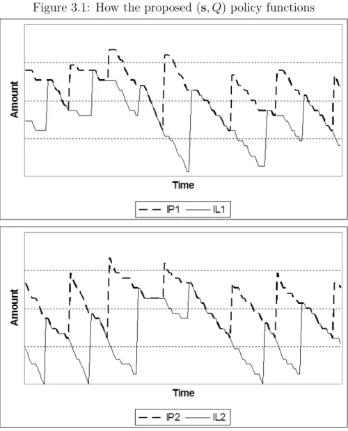
3.1 How the proposed (s, Q) policy functions . . . . 22

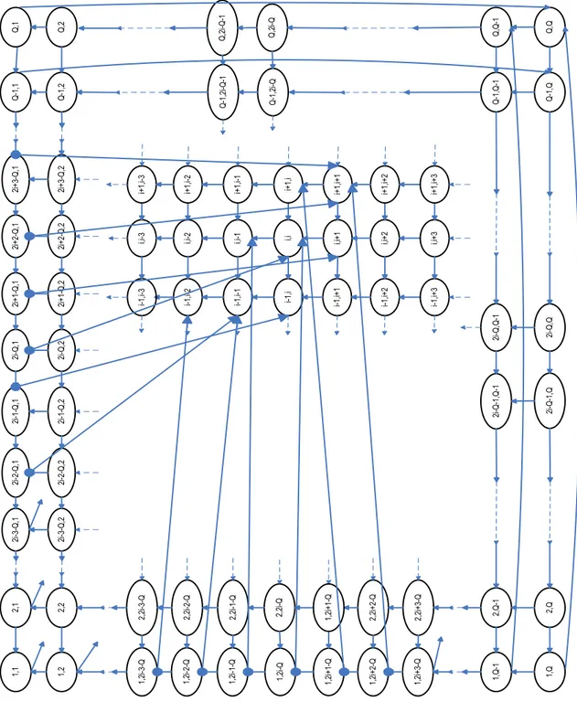
3.2 State transition rate diagram. All transition rates are equal and λ. 27 3.3 Total cost as a function of Q with parameters λ = 5, h = 6, π = 200, K = 150, s = 6 . . . . 28

3.4 Total cost as a function of s with parameters λ = 5, h = 6, π = 200, K = 150, Q = 17 . . . . 29

3.5 Total cost as a function of Q and s with parameters λ = 5, h = 6, π = 200, K = 150 . . . . 30

4.1 Gap(QS) versus C/Q∗ _{values when l = 0.25, π = 20} _{. . . .} ₄₀

4.2 Gap(QS) versus C/Q∗ _{values when l = 0.5, π = 20 . . . .} ₄₀

4.3 Gap(QS) versus C/Q∗ _{values when l = 1, π = 20 . . . .} ₄₀

4.4 Gap(QSs) versus C/Q∗ _{values when l = 0.25, π = 20 . . . .} ₄₁

4.5 Gap(QSs) versus C/Q∗ _{values when l = 0.5, π = 20} _{. . . .} ₄₁

4.6 Gap(QSs) versus C/Q∗ _{values when l = 1, π = 20} _{. . . .} ₄₁

4.7 Gap(QS) versus C/Q∗ _{values when l = 0.25, π = 100 . . . .} ₄₄

4.8 Gap(QS) versus C/Q∗ _{values when l = 0.5, π = 100} _{. . . .} ₄₄

(11)

LIST OF FIGURES xi

4.9 Gap(QS) versus C/Q∗ _{values when l = 1, π = 100} _{. . . .} ₄₄

4.10 Gap(QSs) versus C/Q∗ _{values when l = 0.25, π = 100} _{. . . .} ₄₅

4.11 Gap(QSs) versus C/Q∗ _{values when l = 0.5, π = 100 . . . .} ₄₅

4.12 Gap(QSs) versus C/Q∗ _{values when l = 1, π = 100 . . . .} ₄₅

4.13 Gap(QS) versus C/Q∗ _{values when l = 0.25, π = 300 . . . .} ₄₆

4.14 Gap(QS) versus C/Q∗ _{values when l = 0.5, π = 300} _{. . . .} ₄₆

4.15 Gap(QS) versus C/Q∗ _{values when l = 1, π = 300} _{. . . .} ₄₆

4.16 Gap(QSs) versus C/Q∗ _{values when l = 0.25, π = 300} _{. . . .} ₄₇

4.17 Gap(QSs) versus C/Q∗ _{values when l = 0.5, π = 300 . . . .} ₄₇

4.18 Gap(QSs) versus C/Q∗ _{values when l = 1, π = 300 . . . .} ₄₇

B.1 Gap(QSs) vs π when l=1 . . . . 61 B.2 Gap(QSs) vs π when l=0.5 . . . . 61 B.3 Gap(QSs) vs π when l=0.25 . . . . 62 B.4 Gap(QS) vs π when l=1 . . . . 62 B.5 Gap(QS) vs π when l=0.5 . . . . 63 B.6 Gap(QS) vs π when l=0.25 . . . . 63

(12)

List of Tables

3.1 Summary of Notation . . . 13

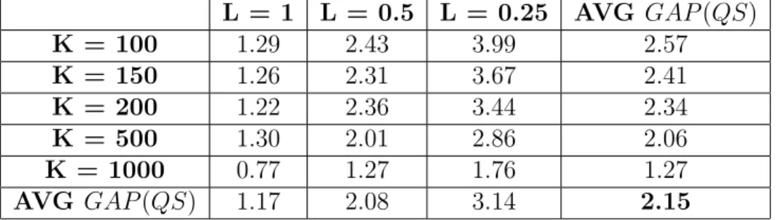
4.1 Average percentage gap between the (Q, S) and the (s, Q) policies over all K values. . . . 33

4.2 Average percentage gap between the (Q, S, s) and the (s, Q) poli-cies over all K values. . . . 34

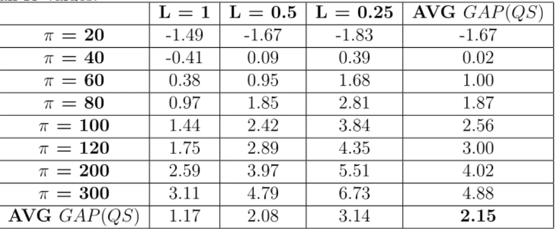
4.3 Average percentage gap between the (Q, S) and the (s, Q) policies over all π values. . . . 35

4.4 Average percentage gap between the (Q, S, s) and the (s, Q) poli-cies over all π values. . . . 36

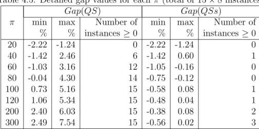
4.5 Detailed gap values for each π (total of 15 × 8 instances) . . . . . 37

4.6 Detailed gap values for each K (total of 24 × 5 instances) . . . . . 37

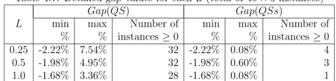
4.7 Detailed gap values for each L (total of 40 × 3 instances) . . . . . 38

4.8 Comparison of the three policies for N = 4 and π = 20 case . . . . 38

4.9 Comparison of the three policies for N = 4 and π = 120 case . . . 38

4.10 Percentage gap between the (s, Q) and the (Q, S) policies for non– identical items . . . 49

(13)

Chapter 1 Introduction

Many companies manage inventories of multiple items. The primary challenge in managing multi–item inventory systems is the fact that some of the costs are incurred jointly. In particular, the setup costs in production, purchasing or transportation are often incurred jointly for the multiple items that are included in the production batch, purchase order or the shipment. Joint setups can be seen as an opportunity as well as a challenge, since scale economies can be exploited to reduce setup costs or reduce cycle inventories or both, by carefully coordinating the replenishment of multiple items. The joint replenishment problem (JRP) is to determine the inventory replenishment policy of multiple items that share a common setup.

A basic example of the joint replenishment problem occurs in a setting where multiple items are sourced from a common supplier. Setup costs in this setting may include the transportation costs and purchase transaction costs. Since 1980s, many manufacturing companies are reducing their supplier bases. Examples in-clude Xerox reducing its supplier base in early 1980s from 5000 to 400 [6], Texas Instruments reducing its MRO suppliers from 5000 to 750 between 1998 and 2000 [24], Merck reducing its total global supplier base from 40,000 in 1992 to fewer than 10,000 in 1997 [15], IBM now using only 50 suppliers for the 85 % of its requirements [9] and Sun Microsystems now using only 40 suppliers for the 90 % of its requirements [8]. Among other things, reduction of the supplier base helps companies decrease their inventory holding, transportation and purchasing costs by giving them the capability of jointly replenishing multiple items from common

(14)

CHAPTER 1. INTRODUCTION 2

suppliers.

Being sourced from a common supplier is not a necessity for jointly replen-ishing multiple items. Companies are devising numerous strategies to leverage economies of scale of combining different items into a single delivery. Among these, the milk–run strategy allows the joint procurement of multiple SKUs from different suppliers located in close physical proximity and helps companies consoli-date smaller shipments to more efficient larger shipments (or move from infrequent independent shipments to more frequent joint shipments) to reduce transporta-tion costs and cycle stocks. For example, Toyota’s Kentucky plant sources 80 % of its parts from suppliers that are located within 200 miles of the plant. Milk–run vehicles serving these suppliers help Toyota receive deliveries on a JIT basis [19]. Another example is Eastman Kodak that significantly increased the frequency of inbound shipments to its plants by successfully implementing the milk–run strat-egy [12]. A final example of milk–run is the commercial vehicle producer MAN. In 2004, MAN’s Ankara plant successfully reduced its inbound transportation costs and component inventory by consolidating its shipments from various compo-nent manufacturers located in close proximity in Northwestern Turkey: a project jointly undertaken by MAN and Industrial Engineering Department at Bilkent University. Another strategy that allows companies to exploit economies of scale in inbound transportation is cross–docking. With cross–docking, smaller ship-ments from multiple suppliers can be merged in a consolidation warehouse for a larger and more economical joint delivery. Cross–docking has been a successful strategy in practice including the famous Wal–Mart implementation [31].

Joint replenishment is also relevant when replenishing a single item in mul-tiple locations. As in the case of multi–item inventory systems, companies are developing strategies that will help them exploit economies of scale of combining shipments to multiple locations under their control. For example, a milk–run vehicle can depart from a supplier or a distribution center and visit a group of production plants to replenish them jointly, reducing the transportation costs and cycle inventories. An example of this is again Eastman Kodak which implements the milk–run strategy for its shipments from its distribution center to multiple plants as well as from multiple suppliers to its distribution centers [12]. Milk–runs are widely used to replenish multiple retail store locations from retailer owned distribution centers or from suppliers directly. Aforementioned cross–docking also enables multiple facilities to consolidate their replenishment at least for a portion

(15)

of the trip. Joint replenishment of multiple locations is possible when all these lo-cations are centrally controlled or when these lolo-cations are in a coalition for joint replenishment. Under a Vendor Managed Inventory contract between a supplier and multiple retailers (or other downstream players), the supplier takes control of the management of inventories at the retail locations. Among other benefits, VMI contracts allow the joint replenishment of multiple retail location and help reduce the transportation and inventory costs for the supply chain ([10], [11]).

In accordance with its relevance and importance in practice, the joint replen-ishment problem has been an extensively studied research topic for almost 40 years starting with the pioneering works of Balintfy [5] and Silver [27]. Formally the problem is to determine the replenishment and inventory policies of N items (or locations) to minimize the total setup, holding and shortage costs in the pres-ence of setup costs that are incurred jointly. In a more general setting, in addition to the setup costs that are common and incurred with each replenishment order regardless of which items are involved (major setups), item specific setup costs may be incurred for each item in the order (minor setups). Research in this area followed two separate paths depending on whether the demands are deterministic or stochastic; the latter being referred to as the stochastic joint replenishment problem (SJRP). In this thesis, SJRP is investigated.

One major gap in the existing literature on the joint replenishment problem is the fact that the setup costs (major or minor) are independent of the size of the order. This may be a reasonable assumption when the setup costs reflect the administrative costs that are related to a purchase order or the production setups that are incurred for a production batch. However, when the setup costs are due to transportation costs (perhaps the main motivation of the joint replenishment problem), such an assumption is rather restrictive. In practice the transporta-tion is carried out with capacitated vehicles. Thus, the setup cost structure is step–wise, each step corresponding to an additional vehicle. Such cost structures are recently being investigated in the literature (see, for example, Alp et. al [2]) for the single item inventory systems. The main contribution of this thesis is the incorporation of the transportation vehicle capacities and associated cost struc-tures for the stochastic joint replenishment problem. In particular, we develop a replenishment policy in which a replenishment order of fixed size (perhaps the capacity of the vehicle) is created whenever the inventory position for one of the

(16)

policy, where s is the vector of reorder points for the N items, and Q is the constant reorder quantity.

A partial motivation for this study is our experience with a beverage producer in Turkey. This beverage producer manages the inventory of its distributors under a VMI like setting and dispatches trucks for the replenishment of about 100 SKUs at each distributor. The trucks that are used for the shipments are capacitated. Since the trucks travel large distances (up to 1000 kilometers), the transportation costs are substantial (as compared to inventory holding costs) and do not depend significantly on the load of the truck, the beverage producer almost always dispatches full trucks to its distributors. The company also wants to maintain a high service level at its distributors at which the demand for the SKUs can be highly uncertain. This rules out a policy that removes the ability of each SKU individually triggering a replenishment order. One such policy is (Q, S) policy, in which a replenishment order of size Q is triggered whenever the total demand since last order reaches Q to bring up the inventory position of the

N items to S.

In the specific setting in which we propose our policy, there are N items (or locations). The demand for each item follows an independent Poisson process. There are no minor setup costs. Unsatisfied demand is completely backlogged. Two types of backlogging costs are incurred: per backlog occasion and based on the backlog duration. Linear inventory holding costs are charged. The problem is to determine the reorder quantity Q and reorder points s so that the total expected ordering, inventory holding and backlogging costs are minimized. When the items are identical, the contents of the replenishment order is decided in a way that item inventory positions are equalized (to the extent that this is possible). For the case of non–identical items, we devise a rule to allocate the fixed replenishment quantity to multiple items based on the stock–out costs. The policy is general in the sense that the same set–up cost can be incurred regardless of the reorder quantity Q. To consider the case of capacitated vehicles, we introduce a capacity C and it is sufficient to consider the case of Q ≤ C, since we have a continuous review model.

We conduct a numerical study to asses the performance of the proposed (s, Q) policy against two policies in the literature. One of these policies is the (Q, S) policy which is described earlier. The second policy is the (Q, S, s) policy in

(17)

which a replenishment order is triggered whenever the total demand since the last order reaches Q or the inventory position of any of the items drops to its reorder point. Our numerical study results show that, there is no dominance relationship between these policies. One policy may outperform the others in different settings. However, when vehicle capacities are assumed to be infinite, the (s, Q) policy tends to outperform the (Q, S) policy while the (Q, S, s) policy outperforms the (s, Q) policy in most of the cases. On the other hand, when vehicle capacities are assumed to be finite, the (s, Q) policy outperforms the other policies in most of the cases considered.

The rest of this thesis is organized as follows. In Chapter 2, we review the lit-erature on the stochastic joint replenishment problem. In Chapter 3, we propose our new policy (s, Q) along with a review of the replenishment policies (Q, S) and (Q, S, s). In Chapter 4, we present our numerical results that compare the three policies when the vehicle capacities are both not considered and considered. Chapter 5 concludes the thesis and suggests some avenues for future research.

(18)

Chapter 2 Literature Survey

In this chapter we review the literature on the stochastic joint replenishment problem. In the first part of the chapter, we focus on the single–echelon inventory systems. These inventory systems are discussed under two categories: periodic review and continuous review. In the second part of the chapter we review multi– echelon inventory systems and vendor–managed inventory systems. While there is a large body of literature on the deterministic joint replenishment problem, we do not review this literature here. For a review of that literature see Aksoy and Ereng¨u¸c [1] and Goyal and Satir [16].

Replenishment policies are vital for an efficient inventory system. When there are multiple items, cost savings can be obtained through jointly replenishing them. The savings through joint replenishment can be substantial, when efficient joint replenishment policies are used. The previous research in this area shows that finding a good solution for the joint replenishment problem is difficult. Ignall [18] studies the replenishment problem to find the optimal joint replenishment policy. The main result of this study is that the optimal policy in joint replen-ishment, even for a two–item case, is complicated because of the dependency of the quantity ordered on inventory levels of two items. As the number of items in the system increases, the inventory system is more difficult to control and the implementation of the joint order policies are even more challenging. Therefore, heuristic policies are sought in the literature.

Balintfy [5] is the first to study the stochastic joint replenishment problem. 6

(19)

CHAPTER 2. LITERATURE SURVEY 7

We begin our survey with this study. Balintfy [5] develops a continuous–review joint ordering policy, which determines the range of reorder points at which several items can be ordered simultaneously. This new policy is suitable for computer– controlled inventory systems. In individual ordering, each item triggers a replen-ishment order whenever its inventory position drops to a certain level, referred to as the reorder point. The replenishment order consists of only the item that triggered the order. For joint ordering, a new quantity called the can–order point is defined. The area between the can–order point and the reorder point is called the reorder range. Items, whose inventory positions fall within this range, are also ordered when an order is triggered.

This new policy by Balintfy [5] is referred to as can–order policy and is repre-sented as (S, c, s). S is the vector of order–up–to levels; s is the vector of reorder points and c is the vector of new points called the can–order point. This new policy functions as follows. An order is triggered when any of the items inventory position drops to or below its reorder point s. When the order is triggered, the inventory position of the item that triggered the ordering is raised to its order– up–to level. Simultaneously, the inventory positions of the other items are also checked. If the inventory position of any of the items is at or below the can–order point, that item’s inventory position is also raised to its order–up–to level. This policy seems to be simple; unfortunately, however, it is difficult to derive cost expressions analytically.

Silver [27] studies a special case of the (S, c, s) policy. In this special case, the replenishment leadtime is zero, c is assumed to be S − 1 and s = 0 for each item. Demands are assumed to be Poisson and shortages are not allowed. The objective is to minimize the expected total cost per unit time, comprised of the holding cost and the ordering cost. Silver [27] proves that the can–order policy performs better than individual ordering if the fixed ordering cost does not change with joint ordering. If the fixed costs are not equal in individual ordering and joint ordering, whether the joint replenishment will reduce the cost depends on the fixed cost for the joint replenishment. If the fixed cost for the joint replenishment lies below a critical value, joint replenishment reduces costs.

Another study on the (S, c, s) policy by Silver [29] who decomposes the N– item problem with unit Poisson demands into N single–item problems to ap-proximate the solution. This single–item problem is first analyzed by Silver [28]

(20)

himself and solved optimally by Zheng [34]. The same decomposition method is used for compound Poisson demand by Thompson and Silver [32] and Silver [30]. When Poisson arrival process for the special replenishment possibilities is assumed, (i.e., the reduced cost occur probabilistically according to a Poisson process with a rate µ per year, where µ is the expected number of orders trig-gered per year by all other items in the group), Van Eijs [33] and Schultz and Johansen [26] show that the decomposition method performs poorly.

Federgruen et al. [14] suggest a semi–Markov decision model and use a de-composition approach similar to Silver [30]. The authors focus on calculating the control parameters of the (S, c, s) policy and propose a heuristic method using a policy–iteration algorithm to find the control parameters. This decomposition approach is different than Silver [30], since it is based on the fact that under general conditions, superpositions of n point processes converge to a Poisson pro-cess as n −→ ∞. Using this approach, the problem becomes an n independent single–item problem.

One of the most important continuous–review control policies for the joint replenishment problem in the literature is the (Q, S) policy. This policy is first proposed by Renberg and Planche [25]. In this thesis, we compare the perfor-mance of our proposed policy and the (Q, S) policy. Pantumsinchai [23] subse-quently studies the policy, assuming Poisson demand. The policy is simple and functions as follows: when the total amount of demand since the previous order has reached Q, an order in the amount of Q is placed with the supplier to raise the inventory positions of all of the items to S. Q is the order quantity and S is the order–up–to level. Pantumsinchai [23] compares the (Q, S) policy with the (S, c, s) policy, and shows that the (Q, S) policy performs better than the (S, c, s) policy if the fixed ordering cost is high and the shortage cost is low. The (S, c, s) policy only performs better if the fixed ordering cost is low.

Cheung and Lee [11] also study the (Q, S) policy, but in a setting with single warehouse and multiple retailers. The policy works similarly with in an inventory system with a single retailer multiple items. In this multi–retailer case, an order is triggered when a total of Q units are demanded in all retailers. After an order is triggered, inventory positions of the retailers are all raised up to their maximum levels S. Cheung and Lee [11] analyze the model exactly in a setting where the warehouse uses the (Q, R) policy for its inventory control. They also propose

(21)

a new model applying the same policy in which the stocking positions of the retailers can be rebalanced while unloading the items and find a lower and an upper bound for this model.

Atkins and Iyogun [3] propose two periodic review replenishment policies and compare them against the (S, c, s) policy. These policies are referred to as (R, T )– type policies. In this class of policies, the inventory is reviewed periodically, and inventory position of each item is raised to level R at the end of each period of length T , by creating a joint replenishment order. The first proposed pol-icy of this kind is called a periodic heuristic polpol-icy and is represented by P . In this policy, the period lengths are identical. The second type is called a

modif ied periodic heuristic policy and is represented by MP . In this policy,

periods are integer multiples of a base period and periods can differ for each item. Computational results illustrate that as the fixed cost increases, P and

MP type policies outperform the (S, c, s) policy. Atkins and Iyogun [3] conclude

that simple periodic policies seem to work better than complicated can–order policies. Pantumsinchai [23] also studies the MP type policy and shows that the performance of MP is comparable to the (Q, S) policy.

A recent study that considers periodic and continuous review policies for the stochastic joint replenishment problem is by Cachon [7]. Ca-chon [7] considers three policies for dispatching trucks; the first one is the

minimum quantity continuous review policy in which the inventory is

re-viewed continuously. Trucks are dispatched, (i.e., a replenishment is triggered) when a total of Q units have been ordered. The order quantity here is equal to Q, which is the demand since the last shipment. The second policy is the

f ull service periodic review policy. In this case, inventory is reviewed every T time units, and trucks are dispatched to replenish the shelves of the stores,

regardless of how much demand has been accumulated since the last order. The third policy is the minimum quantity periodic review policy, which is referred to as the (Q, S|T ) policy. In this policy, the retailer reviews its inventory at every

T time units. Trucks are dispatched when one of the trucks has at least Q units,

and the others are all full.

The final study that we like to discuss under a single echelon setting is a study by Nielsen and Larsen [20]. Nielsen and Larsen propose a new policy referred to as the Q(S, s) policy. This policy functions as follows: when a total amount of Q

(22)

demands are accumulated since the last review, a replenishment order is triggered. Items whose inventory positions in this review at or below s are ordered up to

S. This policy becomes a (Q, S) policy if identical demand and identical cost

structures are assumed for the items. It is shown that this policy performs better than the previous policies under certain settings.

While there is a large body of literature on multi–echelon inventory systems (for a review and two recent models see Axsater [4] and Federgruen [13]), a few number of studies look at the stochastic joint replenishment problem in a multi– echelon setting. One such study is Gürbüz et al. [17]. In this study, the supply chain consists of a cross–dock location which serves multiple identical retailers. A new replenishment is triggered when a total of Q demands are observed, or when a retailer’s inventory position drops to its reorder point. Whenever a replenishment order is triggered, inventory position at each retailer is raised to its order–up–to level. Gürbüz et al. [17] compare the proposed policy with the (Q, S) policy, the periodic review order–up–to policy (S, T ) and the special can–order policy (S, c, s). The numerical results show that the proposed policy is better than the other policies under the settings considered. Also in this paper, the authors compare this policy with the others considering additional transportation penalty costs. These penalty costs are incurred, when the number of units shipped exceed the truck capacity, and the costs are based on per–unit exceeded. The proposed policy also outperforms other policies under such transportation penalty costs.

The most recent study on stochastic joint replenishment problem in literature is by ¨Ozkaya et al. [21]. In this study they propose (Q, S, T ) policy in a single location, N-items setting. This policy functions as follows: a new replenishment is triggered and inventory positions of all of the items are increased up-to their order-up-to points, whenever a total of Q units are demanded or when T time units elapse. In this study, it is shown that the (Q, S, T ) policy outperforms the other joint replenishment policies in most of the problem instances considered. The new joint replenishment policy is studied and its performance is compared against other policies in a two-echelon setting in ¨Ozkaya et al. [22].

A related topic in the multi–echelon setting is the Vendor Managed Inventory (VMI) systems. It is argued that one of the benefits of VMI is the manufacturer’s ability to consolidate shipments to jointly replenish the retailers. This aspect of VMI systems is studied by C¸ etinkaya and Lee [10]. Resupply time and the

(23)

quantity is decided by the supplier using this information and substantial savings are realizable by a consolidation program that combines small shipments to create larger and more economical deliveries. In this program, replenishment orders wait at the warehouse for the allocation of a specific quantity or for a specified time. The authors study the problem from the vendor’s perspective and do not consider the performance of the retailers.

The main contribution of this thesis to the existing literature on the stochastic joint replenishment problem is a new policy that considers the capacity of vehicles that deliver the joint replenishment. We call this policy the (s, Q) policy. In this policy, an order is triggered whenever the inventory position of an item drops to its reorder point s. The order size is always Q. Since we are not maintaining a constant inventory position for each item at the replenishment epoch, the replenishment order has to be allocated to different items. In the symmetric case the replenishment order is allocated to each item such that the inventory positions are equalized (to the extent that this is possible). The policy is designed especially for situations where the replenishments are shipped using capacitated vehicles and individual items have substantial shortage penalties. The policy is compared against the (Q, S) and the (Q, S, s) policies under a variety of settings.

(24)

Chapter 3 Model

We consider a supply chain that consists of a single warehouse, a single retailer and N items. While a single item, multi–retailer problem is equivalent to a single retailer, multi–item problem when the warehouse has ample supply, we use the latter setting throughout the chapter for consistency. The inventories of items are controlled in a continuous and coordinated fashion by the retailer. Items are shipped from the warehouse to the retailer by a fleet of trucks each having a fixed and identical size. The warehouse has an unlimited supply capacity and the fleet size is assumed to be sufficient enabling the dispatch of the items from the warehouse whenever necessary. There is a fixed transit time from the warehouse to the retailer, which corresponds to the replenishment leadtime, L. The notation used throughout the chapter is introduced as need arises and it is also summarized in Table 3.1.

We assume that the demand observed by the retailer for item i follows a Poisson process with a rate of λi and unsatisfied demands are fully

backo-rdered. The holding cost, hi, is incurred at the retailer level per item per

unit time. The backordering cost, πi, is the cost incurred for each unit

back-ordered. The shortage cost, pi is incurred per unit backorder per unit time. The f ixed ordering cost, K, is associated with the use of trucks, i.e., for every truck

of capacity C utilized for shipment, a fixed cost of K is incurred independent of the quantity loaded.

(25)

CHAPTER 3. MODEL 13

λi Arrival rate of the demand for item i at the retailer L Replenishment lead time

K Fixed ordering cost associated to the use of each truck

Si Order up to level of item i at the retailer si Reorder point of item i at the retailer

Di(t) Demand observed at the retailer for item i during a time period of t

C Capacity of a truck

N Number of items in the system

pi Unit shortage cost of item i per unit time

πi Backordering cost of item i per each unit backordered h Unit inventory holding cost per unit time for item i

τ Random variable denoting the time between two consecutive replenishments

f (·) pdf of τ

IPi(t) Inventory position of item i at time t ILi(t) Inventory level of item i at time t

∆i Si− si

Table 3.1: Summary of Notation

The retailer aims to find a joint replenishment policy for the inventory man-agement of her N items to minimize the total holding, backordering and the fixed costs of ordering in this particular environment. In literature, there are two dif-ferent heuristic policies (the (Q, S) policy of Cachon [7] and the (Q, S, s) policy of G¨urb¨uz et al. [17]) proposed for this problem. In this thesis, we propose a new heuristic policy which we refer as the (s, Q) policy. Next, we present the detailed explanation of these policies.

3.1 The (Q, S) policy

This policy is first suggested by Renberg and Planche [25] for the general joint replenishment problem. The policy under Poisson demand is studied by Pan-tumsinchai [23]. The policy under a capacitated vehicle is studied by Cachon [7]. In this policy, when the total amount of demand since the previous order reaches Q units, an order in the amount of Q is placed so that the retailer raises the inventory positions of all items up to the vector S = (S1, S2, ..., SN), where Si is the order–up–to level of item i. That is, when the total inventory position

(26)

IP (t) =PN_i=1IPi(t) drops to ST − Q, where ST =

P_N

i=1Si, an order amount of Q is placed to raise the inventory positions of all items up to their order–up–to

level Si. ST − Q can be assumed as the system reorder point. Since fixed cost

of K is incurred every time a truck is utilized, delaying the shipment of a fully loaded truck will not be optimal under a (Q, S) policy. Hence, when optimizing the policy parameters, one should search the region [1, C] for the optimal value of Q for any given truck capacity, C.

Pantumsinchai [23] presents the derivation of the total expected cost function of this policy. Since all of the inventory positions are raised to their order– up–to points, Si, whenever an order is triggered, inventory positions become a

regenerative process. Therefore, the inventory positions of items reach to a steady state and their limiting probability can be computed. The cumulative demand for an item since the last order is binomially distributed for given cumulative demand for all items. If we let Xi be the random variable for the cumulative demand since

the last order for item i and X0 be the

P_n

i=1Xi, P (Xi|X0) becomes binomial

with parameters x0 and θi, where θi = λi/λ0, where x0 is uniformly distributed

between 0 and Q − 1. Therefore, the marginal distribution of Xi, referred to as u(xi) becomes: u(xi) = 1 Q Q−1 X x0=xi Ã x0 xi ! θxi_{(1 − θ)}x0−xi_, _x i = 0, 1, ..., Q − 1, as shown in Pantumsinchai [23].

It can be shown using recursive calculations that the marginal distribution of

Xi is given by:

u(xi) = 1

θQ(1 − B(xi; Q, θ)), xi = 0, 1, ..., Q − 1,

where B(xi; Q, θ) is the cumulative binomial probability. The expected value of Xi is θ(Q − 1)/2 and the variance is θ(1 − θ)(Q − 1)/2 + θ2(Q2− 1)/12.

In order to calculate different cost components, we should first calculate the stockout probabilities and the expected backorder size at any time. Therefore, we should know about the inventory positions and the net inventories of the items. It is known that the inventory position at any time t depends on the fixed lead time L. Assuming that the inventory position of an item is z at time t − L and

(27)

the demand for the item between t − L and t is di, the net inventory at any time t becomes z − di = S − v where v = xi+ di. This is because, items ordered before

time t − L will be on hand by time t but the items ordered after time t − L will not be on hand by time t. If we let m(v) be the probability distribution of v,

m(v) becomes:

m(v) =

min(v,Q−1)_X x=0

u(x)r(v − x), v = 0, 1, 2, ...,

where r(.) is the probability of demand during lead time.

We now can calculate the stockout probability and expected size of backorder at any time. If we let P (S, Q) be the stockout probability and B(S, Q) be the expected size of backorder at any time, then the equations become:

P (S, Q) = P r(v ≥ S) = ∞ X v=S m(v), and B(S, Q) = ∞ X v=S+1 m(v).

For the calculation of the expected backordering cost, we need to know the av-erage stockouts per unit time which is represented by λP (S, Q) and the expected number of stockouts which is represented by P_iPi(Si, Q). For the calculation

of the holding costs, we use the expected on hand inventory which is equal to

S − θ(Q − 1)/2 − λL + B(S, Q). With all this information, it is straightforward

to write the expected total cost equation per period. If we let C(Q, S1, ..., Sn) be

the expected total cost per period, the equation becomes:

C(Q, S1, ..., Sn) = Kλ0 Q + n X i=1 hi(Si− θi(Q − 1)/2 − λiLi) + n X i=1 (pi+ hi)Bi(Si, Q) + n X i=1 πiλiPi(Si, Q).

3.2 The (Q, S, s) policy

In this section, we present the details of the (Q, S, s) policy suggested by G¨urb¨uz et al. [17]. In this policy, when the total amount of demand since the previous

(28)

order reaches Q or whenever any of the item’s inventory position drops to its reorder point si, the inventory positions of each item at the retailer are raised

to their corresponding order–up–to levels. Hence, there are two different ways of replenishing the system. The first way is only related individually to the retailer’s inventory position; that is, whenever any of the retailer’s inventory positions drops to its reorder point, replenishment occurs. The second way is related to the total echelon inventory position. Whenever the inventory position of the total echelon drops to PN_i=1Si− Q, replenishment occurs. Here, if Si − si ≥ Q for all i, then

this policy works as a (Q, S) policy.

G¨urb¨uz et al. [17] present exact expressions of the total expected costs realized in this policy in the case of identical items. Since the inventory positions are raised to the same level, at every replenishment epoch, we have a regenerative process as in the case of (Q, S) policy. As a result, inventory positions of the items reach a steady state. The time between two consecutive orders is called the cycle time and is represented by τ . In order to calculate the expected ordering cost, we first need to find the expected cycle time. Therefore, it is necessary to calculate the probability density function of τ . Let ∆ = S − s, then due to the policy requirements

τ = min(T1

∆, ..., T∆N, TQ),

where Ti

∆ ∼ Erlang(∆, λ) for all i and TQ ∼ Erlang(Q, N λ).

Here, Ti

∆ is the time at which ∆th demand occurs at the retailer i and TQ is

the time when a total number of Q units is demanded within the system. TQ

would be the cycle time, only if the total demanded amount within the system reaches Q before any of the retailer’s inventory positions drops to s. The cycle time is greater than t, if the retailer’s inventory positions did not drop to s and the total system demand did not reach Q by that time. Therefore, the cumulative distribution function of the cycle time is driven by the following equation:

Fτ(t) = P r(τ ≤ t) = 1 − P r(τ > t) = 1 − P r(D1(t) ≤ ∆ − 1, ..., DN(t) ≤ ∆ − 1, D0(t) ≤ Q − 1) = 1 − (∆−1)Λ(Q−1)_X d1=0 (∆−1)Λ(Q−1−dX 1) d2=0 ... (∆−1)Λ(Q−1−dX1−...−dN −1 dN=0 N Y i=1 p(di; λt),

(29)

where D0(t) =

P_N

i=1Di(t). and Di(t) is the demand to retailer i for a period of t

time units.

The probability density function of the cycle time τ is calculated by taking the derivative of the cumulative function above and represented by the following equation: f (t) = Nλ (∆−1)Λ(Q−1)_X d1=0 (∆−1)Λ(Q−1−dX 1) d2=0 ... (∆−1)Λ(Q−1−dX1−...−dN −2) dN −1=0 × N −1_Y i=1 p(di; λt)p((∆ − 1)Λ(Q − 1 − d1− ... − dN −1); λt).

The equation above reveals that the distribution of the cycle time depends only on Q and ∆. This distribution is used to calculate the ordering cost.

To calculate the other cost components–holding costs and backordering costs– the probability distribution of the inventory level should be known. To derive the inventory level distribution, the random demand distribution is needed. When

Q > ∆ + (N − 1)(∆ − 1), the total system demand will never reach Q before any

of the item’s inventory positions drops to s. Therefore, for this case we have,

P (Di ≥ n) =        1 if n = 0 R_∞ t=0λp(n − 1; λt)[1 − P (∆; λt)](N −1)dt if 1 ≤ n ≤ ∆ − 1 0 if n ≥ ∆ where P (r; µ) =P∞_j=rp(j; µ) and p(j; µ) = e−µ µj j!.

When Q ≤ ∆ + (N − 1)(∆ − 1), an order can be triggered in either way. The probability distribution of the amount shipped to the retailer during a cycle time, represented by Zi, is the following:

(30)

CHAPTER 3. MODEL 18 P (Z ≥ n | Q, ∆, N ) =                                  P (Z ≥ n | Q − 1, ∆, N ) + φ(Q, ∆, N ) if n = 0, 1, ..., Q − 1 P (Z ≥ n | Q − 1, ∆, N ) + φ(Q, ∆, N )

if n = min(∆, Q)& min(∆, Q) = min(∆, Q − 1) P_n−1 d1=n−1... P_{(∆−1)Λ(Q−1−d}₁_−d₂_−...−d_{N −1}₎ dN=0 h(d1,d2,...,dN) N

if n = min(∆, Q)& min(∆, Q) > min(∆, Q − 1) where D0 = N X i=1 di, h(d1, d2, ..., dN) = Do! ND0 ×QN i=1di! , and φ(Q, ∆, N) = λ Ã Q − 1 n − 1 ! µ 1 N ¶_n−1µ 1 − 1 N ¶_Q+1−n × (E(τ |Q + 1 − n, ∆, N − 1) − E(τ |Q − n, ∆, N − 1)). These equations suggest calculating the probability of Z recursively.

The relationship between the inventory position and the inventory level is

IP (t − L) − D(L) = IL(t), where IL(t) is the inventory level at time t, and IP (t − L) is the inventory position at time t − L. To calculate the holding costs

and backordering costs, we should find the inventory level distribution using the inventory position distribution. The inventory position distribution is derived using demand distributions. For Q = 1,

P (D ≥ n | Q) = ( 1 if n = 0 0 if n ≥ 1 , and when Q ≥ 2, P (D ≥ n | Q) =        1 if n = 0 P (Z ≥ n | Q − 1) if 1 ≤ n ≤ min(∆ − 1, Q − 1) 0 if n ≥ min(∆, Q) .

(31)

Since the demand distributions are known, the inventory position distribution can easily be calculated. The equation for the inventory position distribution can be found as follows: P r(IP = j) = (∆−1)Λ(Q−1)_X n=S−j P (IP = j | D(τ ) = n)P (D(τ ) = n) = (∆−1)Λ(Q−1)_X n=S−j P (D(τ ) = n) n + 1 , j = S − min(∆ − 1, Q − 1), ..., S.

By using these distributions, the expected value of the cycle time and the expected value of the inventory level can be calculated. These expectations are used to determine the expected ordering cost, the expected holding cost and the expected backordering cost. The total cost function is:

CR = K E[τ ] + N × [(h + p)E[IL +_{] + p(E[D(LT )] − E[IP ])} _(3.1) + π × λ(1 − S X j=(max(S−Q+1,S−∆+1))+ j−1 X l=0 p(l, λLT )P r(IP = j))].

G¨urb¨uz et al. [17] use only one type of backordering cost: no backorder costs are charged per occasion, i.e. per unit backordered. However, in Equation 3.1 above, we also incorporate the backorder costs per occasion.

3.3 The proposed (s, Q) policy

In the proposed (s, Q) policy, a joint replenishment order of size Q is trig-gered when the inventory position of an item falls to its reorder point si. Here

s = (s1, s2, ..., sN) denotes the vector of the reorder points of items. The total

order size, Q is then allocated to the items so that their inventory positions are equalized to the extent that is possible. This is achieved by employing the fol-lowing procedure when all items are identical: First, the inventory position of the item which triggered the ordering with the minimum inventory position is increased up to the inventory position of the next item with the lowest inventory

(32)

position and their inventory positions are equated if Q is sufficient. Otherwise all

Q units are allocated to the first item. Next, we begin to increase the inventory

positions of these two items up to the inventory position of the next item with the lowest inventory position and equate their inventory positions (again if Q is sufficient). This process continues in the same manner until a total amount of Q is allocated. Different than the previous policies, the inventory positions at each replenishment epoch are not necessarily equal to each other and there is no fixed order–up–to point for any of the items.

Deciding how to allocate the items is a critical issue in this policy. We employ different allocation rules depending on whether the items are identical in their backordering costs or not. When items are identical, we try to equate their inventory positions as the size of Q permits as explained above. When items are not identical we allocate the total order size of Q to items, by minimizing the total expected backordering costs in the subsequent replenishment cycle. In particular, for each of the items, we calculate how much we save from expected backordering cost in the subsequent replenishment cycle if we increase the inventory position of that item by one unit. We compare the savings and allocate one unit to the item which produces maximum savings. The same procedure is employed until all Q units are allocated. The expected backordering cost of item i with an inventory position of IPi can be calculated as:

EBC(IPi) = πi.E[max{Di(L) − IPi, 0}] = πi ∞

X

i=Ii

(Di(L) = i)(i − IPi).

Specifically, for every item i, we calculate

EBC(IPi+ 1) − EBC(IPi),

and allocate one unit to the item which will provide the highest difference (highest reduction in cost). Note that this allocation rule is merely a heuristic rule. Several different allocation rules may be employed in this setting.

There are some advantages of Q being constant. Since we are using capac-itated vehicles for shipment, companies prefer attaining stable and acceptable utilization levels on the trucks that they dispatch. Moreover, Q being constant, together with the allocation policy explained above, ordering items which have higher inventory positions can be avoided. Since, the truck capacities are con-stant and every time a truck is used a fixed cost of K is incurred, the decision

(33)

on the value of Q will be based on how much of the capacity is utilized. Note that, delaying the shipment of a fully loaded truck cannot be optimal under the (s, Q) policy, similar to the previous policies. Hence, one should search the region [1, C] for the optimal value of Q for any given truck capacity, C. In the (Q, S) policy, an order may include items with unnecessarily high inventory positions since there is no individual control of items. Whereas in our proposed policy, the existence of reorder points allows for such an individual control and hence prevents unnecessarily increasing of those items that already has higher inventory positions. Therefore, the total system saves from total expected holding costs and saves from total expected backordering costs by ordering from the items which have lower inventory.

Figure 3.1 shows how the proposed (s, Q) policy functions. There are two identical items in the system. It can be observed from the graph that when an order is triggered the inventory positions of the items are increased in a way that their inventory positions are equalized. This reduces holding costs since, we do not order much for the item which already has a high inventory position.

The inventory positions of items under the (s, Q) policy can be modeled by a continuous time Markov chain. First, we explain this modeling approach for an identical items case. Due to the nature of the policy and the allocation rule employed, the inventory position of each item can take a value between (s + 1, s + 2, ..., s + Q) at any given time. Let x = (IP1, IP2, ..., IPN) be the vector

of inventory positions of all items at any given time. A continuous time Markov chain model can be constructed by defining its states by the vector x. Since the inventory position of each item can take Q different values and we have N items, this Markov chain has QN _{states. One can find the transition rates from}

every state to each other by considering the demand process. The system leaves its current state when one of the items observe one unit of demand. Since the demand of each item is Poisson with rate λi, the interarrival times of demand

realizations for each item is exponentially distributed with the same rate λi.

Hence, the time that the system stays at any given state is determined by the minimum of these interarrival times, and thus, is exponentially distributed by rate

N

X

i=1 λi.

(34)

(35)

system leaves the current state due to item i) is

λi

P_N

i=1λi .

Thus, the rate of moving from state (IP1, IP2, ..., IPi, ..., IPN) to

(IP1, IP2, ..., IPi− 1, ..., IPN) is λi P_N i=1λi × N X i=1 λi = λi.

An example state transition rate diagram is illustrated in Figure 3.2 for an iden-tical two–item environment with s1 = s2 = 0.

From Figure 3.2 it can be seen that, when a demand occurs for any of the items, the state of the Markov chain will change. Since there are two items, there are two possible ways out from each state as demand arrives to one of the items. Let the current state of the system be (IP1, IP2). When item 1 observes one unit

of demand at the retailer, the state of the system moves to (IP1− 1, IP2) with

rate λ1 if IP1−1 6= s1. If IP1−1 = s1, a replenishment order of size Q is initiated

and this order is allocated to both items by the allocation rule described above. Hence, the state that the Markov chain jumps to depends on the allocation rule and the values of the current state variables. Note that the allocation rule for identical items suggests equating their inventory positions as far as Q permit. Therefore, when there are only two items, the Markov chain enters to a state where inventory positions are equal or to a state where the difference between inventory positions are only one after leaving the current state. For example, when a demand occurs at state (1, 2i + 1 − Q) for item 1, the inventory position of item 1 falls to its reorder point (s1 = 0) and it triggers the ordering. First

the allocation rule increases the inventory position of item 1 up to 2i + 1 − Q after which only Q − (2i + 1 − Q) = 2Q − 2i − 1 units are left to allocate. Since the items are identical, half of the units are allocated to item 1 and the other half is allocated to item 2. As a result, inventory position of each item should be 2i + 1 − Q + 2Q−2i−1₂ = i + 1

2. However, since item 1 triggered the ordering and

we could not have half of an item, we allocate one additional unit to item 1 by integrating the fractional parts. Hence, Markov chain enters the state (i + 1, i). Note that the total of the inventory positions of the two items at the entered state is greater than Q. Otherwise, there is only two possible ways in to that state from the states (i + 2, i) and (i + 1, i + 1). Since the items are identical, state transition procedure is the same for item 2.

(36)

After writing all of the transition equations we calculate the steady state probability distributions. Steady state distribution of the inventory positions can be used to calculate the steady state distribution of the inventory level of the items. Inventory level probabilities are used to calculate the expected backorder-ing and the holdbackorder-ing costs per unit time. Let P {IP = y} denote the steady state probability that inventory position of item i is y at any given time. Then,

P {IL = x} = s+Q

X

i=s+1

P {IP = i}P {Di(L) = x + i},

where Di(L) is Poisson distributed with rate λ × L. Therefore, the expected

backordering cost for an item becomes

EBC = π −1

X

x=−∞

P (IL = x),

and the expected holding cost for an item becomes

EHC = h s+Q

X

x=1

P (IL = x).

The expected ordering cost for an item is

EOC = Kλi

Q .

Therefore, since there are N identical items, the total expected cost becomes

ET C = N × (EOC + EBC + EHC).

The equations of the steady state probabilities, when there are N identical items in the inventory, can be found in Appendix A. Next, we provide the equations when there are two identical items. Since the items are identical λ1 = λ2

and s1 = s2 = s.

The steady state probabilities can be found by solving the set of equations below. The left hand side of the equations are the outgoing rates while the right hand side is the ingoing rates for a state.

2Π(s+Q−i)(s+Q) = Π(s+Q−i+1)(s+Q) for i = s+2,...,(s+Q-1)

(37)

The first two equations are for the states when one of the items inventory position is at its maximum value Q and the difference between the inventory positions is at least 2 units.

2Π(s+Q)(s+Q−1) = Π(s+Q)(s+Q)+ Π(s+1)(s+Q−1)

2Π(s+Q−1)(s+Q) = Π(s+Q)(s+Q)+ Π(s+Q−1)(s+1)

The two equations above are for the states when the difference between in-ventory positions of the items is only 1.

When the inventory positions of the items are at their maximum the equation becomes:

2Π(s+Q)(s+Q) = Π(s+Q)(s+1)+ Π(s+1)(s+Q).

For the rest of the states, we have a set of equations that can be expressed using the following algorithm:

for i = s + 1, ..., (s + Q − 1) for j = s + 1, ..., (s + Q − 1)

if |i − j| = 1 and 2i > Q

2Π(i)(j) = Π(i+1)(j)+ Π(i)(j+1)+ Π(s+1)(i+j−Q)

2Π(j)(i) = Π(j+1)(i)+ Π(i)(j+1)+ Π(i+j−Q)(s+1)

2Π(i)(i) = Π(i+1)(i)+ Π(s+1)(2i−Q)+ Π(2i−Q)(s+1)+ Π(i)(i+1)

else

2Π(i)(j) = Π(i+1)(j)+ Π(i)(j+1)

next j next i

There are totally Q2 _{equations above. Also we have} PQ

i=1

P_Q

j=1Π(i)(j) =

(38)

distributions, Π(i)(j).

The modeling approach explained above can also be extended to a non-identical items setting. In this case, the allocation rule employed plays a critical role. Indeed, the state transition rates are exactly the same as in the non-identical items case, but the state reached from a boundary state (a state with having at least one of the IPi values equal to si + 1) depends on the allocation rule

em-ployed. Note that a replenishment decision is made at a boundary state whenever an item with IPi = si+ 1 observes one unit of demand. First, one can come up

with an algorithm that determines the state to be reached from a boundary state for any given allocation rule. Then, a Markov chain can easily be constructed by using the state transition rates and the output of such an algorithm; and the steady state analysis can be employed similar to the identical items case. We also point out that the modeling framework of (s, Q) policy differs from that of other two policies because the inventory positions of items in the (s, Q) policy do not form a regenerative process as there are no fixed order–up–to levels of items.

After finding the steady state probabilities, we search for the optimal s and

Q values to minimize the expected total cost. Since the steady state probabilities

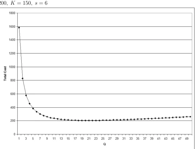
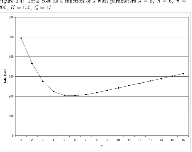
are dependent only on Q for any s, we calculate these probabilities for a given Q only once. Then using these steady state probabilities we calculate the holding and backordering costs, therefore we search for s for given Q that minimizes the expected total cost. Our numerical studies show that the expected total cost seems to be quasi–convex in s for a given Q, which can be seen in an example in Figure 3.4. Also, the expected total cost seems to be quasi–convex in Q for a given s, which can be seen on an example in Figure 3.3. However, we were not able to show this analytically. Figure 3.5 shows the total cost as a function of Q and s for a particular problem instance.

(39)

(40)

Figure 3.3: Total cost as a function of Q with parameters λ = 5, h = 6, π = 200, K = 150, s = 6

(41)

Figure 3.4: Total cost as a function of s with parameters λ = 5, h = 6, π = 200, K = 150, Q = 17

(42)

CHAPTER 3. MODEL 30 Figure 3.5: T otal cost as a function of Q and s with parameters λ = 5, h = 6, π = 200 , K = 150

(43)

Chapter 4 Numerical Study

In this chapter, we compare the performance of the proposed (s, Q) policy to that of the (Q, S) and (Q, S, s) policies through a numerical study. The comparison is based on the optimal total cost rates of the three policies for several problem instances with different parameters including backordering costs, holding costs, fixed ordering costs, number of items, and the capacity of the trucks.

In Chapter 3, we present the total cost rate functions of each policy in terms of their corresponding policy parameters. For each of the three policies and for every problem instance considered, we find the optimal policy parameters by evaluating the total cost rate functions for a sufficiently wide range of parameter values and selecting the ones that minimize the overall cost rate. Even though we present an exact algorithm based on a Markov chain analysis to calculate the total cost rate function of the (s, Q) policy in Section 3.3, the numerical solutions presented in this chapter for (s, Q) policy are found via a simulation study. We make one replication with a run length of 100,000 time units. We verified that this run length is sufficiently long by comparing our simulation results to the exact solution. We initiate the system in a way that the inventory level and the inventory position of each item is equal to s and s+Q, respectively. Finally, note also that the optimal parameters for each policy may turn out to be different than each other in any given problem instance.

Let T C∗

(s,Q), T C(Q,S)∗ and T C(Q,S,s)∗ denote the optimal cost rates of the (s, Q),

(Q, S) and (Q, S, s) policies, respectively. We define the following two functions 31