RESEARCH ARTICLE
Utilizing maximal frequent itemsets
and social network analysis for HIV data analysis
Yunuscan Koçak
1, Tansel Özyer
1and Reda Alhajj
2*Abstract
Acquired immune deficiency syndrome is a deadly disease which is caused by human immunodeficiency virus (HIV). This virus attacks patients immune system and effects its ability to fight against diseases. Developing effective medicine requires understanding the life cycle and replication ability of the virus. HIV-1 protease enzyme is used to cleave an octamer peptide into peptides which are used to create proteins by the virus. In this paper, a novel feature extraction method is proposed for understanding important patterns in octamer’s cleavability. This feature extraction method is based on data mining techniques which are used to find important relations inside a dataset by compre-hensively analyzing the given data. As demonstrated in this paper, using the extracted information in the classification process yields important results which may be taken into consideration when developing a new medicine. We have used 746 and 1625, Impens and schilling data instances from the 746-dataset. Besides, we have performed social network analysis as a complementary alternative method.
© The Author(s) 2016. This article is distributed under the terms of the Creative Commons Attribution 4.0 International License (http://creativecommons.org/licenses/by/4.0/), which permits unrestricted use, distribution, and reproduction in any medium, provided you give appropriate credit to the original author(s) and the source, provide a link to the Creative Commons license, and indicate if changes were made. The Creative Commons Public Domain Dedication waiver (http://creativecommons.org/ publicdomain/zero/1.0/) applies to the data made available in this article, unless otherwise stated.
Background
Acquired immune deficiency syndrome (AIDS) is a deadly disease which is caused by human immunodefi-ciency virus (HIV). This virus destroys immune cells and yields patient’s body to become slowly defenseless against other diseases. According to Global Health Observatory (GHO) report, 78 million people are infected with HIV and it caused the death of 39 million pe ople. As of 2013, nearly 35 million people are living with HIV/AIDS and the mortality is 1.5 million [1]. There are various attempts to keep the virus under control. Unfortunately, effective cure has not been found yet despite the efforts to fully understand how the disease advances and its causes [2]. Inhibitors have been developed to keep it under control.
HIV-1 protease enzyme is used by the virus to cleave an amino acid octomer into peptides which are used to create essential proteins. These proteins are used by the virus to reproduce itself. Spread of the virus in the body is currently blocked with protease inhibitors. Herein, the main issue is to understand the link between HIV-1 protease and amino acid octomer for cleavage. Drugs
become more of an issue during the therapy. Inhibitors mimic a peptide such that chemically modified peptide and scissile bond cannot be cleaved [15].
Available medicines work as HIV-1 protease inhibitors [3], i.e., the aim is to slow down reproduction of the virus. To design better inhibitors, it will be beneficial to find out amino acid sequences can be cleaved by HIV-1 protease [4]. This remains a difficult situation due to the uncer-tainty in patterns for cleavage sites of enzymes.
Amino acid residues are denoted by P4, P3, P2, P1, P1′, P′2, P3′, P′4 and their counterparts in protease are denoted by S4, S3, S2, S1, S1′, S2′, S3′, S′4.
There are 20 possible amino acids which align to make an octamer. This leads to 208 potential combinations of sequences. Data can be encoded in different ways. Although there are two alternative encoding schemes, namely OETMAP [5], and GP [6] encoding, it was noted in recent study by Rögnvaldsson et al. [13] that advanced feature encoding and selection schemes do not lead to better achievement in comparison to standard orthogo-nal encoding in samples without feature selection. A dif-ferent Fresno-style approach was demonstrated by Liao et al. [29] who used Fresno semi-empirical scoring func-tion to predict MHC molecule-peptide binding. Standard orthogonal encoding in representation has 160 binary
Open Access
*Correspondence: [email protected]
2 Department of Computer Science, University of Calgary, Calgary,
Canada
positions (i.e., 20 × 8). While representing an octamer, out of 160 binary values, at each 20 bit length segment, one of them has value one to indicate an amino acid for the octamer. Hence, in total eight bits are set to one and 152 bits have value zero.
The problem of cleavage prediction resorts to binary classification from computational point of view. Recently, a consistency based feature selection mechanism asso-ciated with linear SVM has been proposed for the 746 dataset. Although there are several datasets as completely described in [13], some patterns for cleavage have been elicited particularly in the 746-dataset. In addition to SVM methods, neural networks [7] and markov models have been proposed in the literature. Another direction is introducing extra features by applying machine learning techniques. These techniques have been detailed in [13].
In this paper, we incorporate maximal frequent itemset mining to extract new features for cleavage prediction. These features have been added with different options to fully understand performance compared to results that use stand-alone standard encoding scheme. We alternatively utilize mining results for selected features which were previously named for the 746-dataset. Thus, we facilitate the use of social network analysis in feature selection. A social network graph is constructed based on results of the mining process. This forms a graph based on relationships among items (maximal frequent items). Actually, the power of social network analysis has been increasingly realized and the technique has gained huge interest in the research community. It became very popu-lar in multi-disciplinary domains. Social network analy-sis focuses on relationships among social entities. The proposed methodology has been tested and the results reported in this paper demonstrate its applicability and effectiveness.
The rest of this paper is organized as follows. “The necessary background” section covers the background necessary to understand the approach described in this paper. In particular, we provide a brief overview of net-work analysis, fundamental definitions of frequent pat-tern mining and maximal frequent itemset mining. The proposed methodology is presented in “The methodol-ogy” section. Experiments and the analysis are discussed in “Experiment results and discussion” section; further, patterns specific to the 746-dataset have been used by using social network analysis. “Comparison of algorithms without feature selection” section is conclusions.
The necessary background
The methodology described in this paper integrates tech-niques from social network analysis and data mining which are briefly covered in this section. We use frequent
pattern mining to construct a network between various molecules.
Social network analysis
A social network reflects connections between a set of items inspired from the investigated domain and called actors. Connections are determined based on the type of relationship to be studied and this may lead either to directed or to undirected network. A network may be analyzed based on existing actors and connections to reveal certain discoveries which may be valuable for effective and informative decision making.
Network analysis metrics includes a variety of meas-ures which investigate various aspects of a given network. These include: (1) Degree centrality which is computed differently for directed and undirected networks. For the former, each node has in-degree and out-degree which are, respectively, number of links directed to and out of the node. For the latter, each node has a uniform degree which is the number of links connected to the node. (2) Betweenness centrality which is the number of shortest paths passing through a given node. (3) Density is the ratio of the number of links existing in a graph to the number of links in a complete graph, i.e., maximum den-sity is one. (4) Eigen-vector centrality which determines how popular a given node is.
Frequent patterns
Given a set of items. say I, it is possible to have various not necessarily disjoint subsets of I such that items in each subset are associated based on their coexistence in a given number of transactions where each transaction is a non-empty subset of I. Studying all associations across all subsets could reveal valuable information that describe some implicit relationships between various items. Items associated in a reasonable number of the given subsets form a frequent itemset. For instance, given genes in a body may be differently expressed in a number of sam-ples forming different sets of expressed genes, one set per sample. These sets of expressed genes do overlap and ana-lyzing them would lead to subsets of genes co-expressed together in a large number of samples. It is possible to determine a number of association rules from each fre-quent itemset by splitting the set into two non-empty disjoint subsets of the given itemset such that one sub-set forms the antecedent of the rule and the other subsub-set forms the consequent of the rule. For instance, given a set of samples where only genes expressed in each sam-ple are specified. S1:g1, g2, g3, g5, g6, S2:g1.g3, g4, g5, g7, S3:g2, g3, g6, g8, and S4:g1, g3, g4, g8, g9. From these four samples, it is possible to find some frequent itemsets of co-expressed genes by assuming a minimum threshold
value of 2, i.e., a set of genes is frequent if its genes coex-ist in at least 2 samples. An example frequent itemset could be {g1, g3, g4}, {g2, g3}, etc.
Association rule mining has been well-studied in the literature [10]. Frequent itemsets are prominent for capturing intrinsic structure of a dataset. Formally speaking, given T = t1, t2, . . . , tn as a dataset of n trans-actions, where each transaction ti contains items, e.g., ti = {Ii1, Ii2, . . . , Iik} and each item Iij∈I the set of all possible items. An itemset, IS which contains items from
I, is said to be frequent if and only if it is subset from a
number of transactions in T greater than or equal to a pre-determined minimum support threshold value
(min-sup). Finally, given a set of items F an association rule is
formally defined as X → Y such that X Y = F, X �= φ , Y �= φ and X Y = φ. An itemset F is characterized by support which is defined as the percentage of transac-tions from which F is subset. Further an association rule X → Y has a confidence value which is determined the fraction or ratio of support of X Y by support of X. Minimum support (minsup) and minimum confidence (minconf) threshold value are used in the minimg process for generating association rules that can be derived from
F. Formally, support formula of itemset F is:
where |T| is the total number of transactions. Itemset F is said to be frequent if and only if:
Frequent(F) = F ⊆ I ∧ support (F ) ≥ minsup. Fur-ther, an association rule X → Y is said to be of specific importance when its confidence score is greater than or equal to minimum confidence value. Confidence formula is:
Frequent itemsets can be alleviated to different forms such as closed frequent itemsets [12] and maximal fre-quent itemsets [11]. A frequent itemset is closed if none of its supersets has its support. Formally,
An itemset F is maximal, if it is frequent and none of its supersets is frequent. This can be formalized as:
Closed frequent and maximal frequent itemsets are two concise classes of itemsets which could be used to produced some valuable knowledge in a more controlled and efficient way as described in this paper.
support(F ) = # of transactions having F |T |
confidence(X → Y ) = support(F) support(X)
ClosedItemset(F ) =Frequent(F) ∧ ∀Z((Z ⊃ IS) ∧ (support(F ) �= support(Z)))
MaximalFrequentItemset(F ) =Frequent(F) ∧ ∀Z((Z ⊃ F ) ∧ (frequent(Z) = False))
The methodology
Our methodology is organized in four phases. The first phase transforms the original input data by using orthog-onal encoding. The second phase utilizes the new repre-sentation to find frequent itemsets from the new data representation. The third phase includes selecting the required itemsets from the obtained frequent itemsets. Finally, the selected itemsets are considered as features for classifying instances. Also as a complementary analysis, important itemsets are found by applying social network analysis metrics on a network among existing itemsets.
Data modification
The methodology starts by transforming the original data into orthogonal encoding. In order to find frequent item-sets based on sequences of amino acid octomers, each amino acid is also changed to represent its position on the octomer. For example, the first instance of Schilling Dataset [17], namely
has been transformed into
In orthogonal encoding, there are 8 features for each instance and each feature can have 20 different values, one for each possible amino acid.
Finding frequent itemsets
After transforming the dataset into the new representa-tion, frequent itemsets based on the sequential amino acid octomer can be found. The FP-Growth algorithm has been used to extract frequent itemsets which are above a certain support threshold [18, 19]. In this study, maximal frequent itemsets have been extracted. Maximal frequent items give us a summarization of the given data-set. It is a lossy compression in the sense that all subsets of maximal itemsets are also frequent, but the support value of each subset itemset is not known.
In our experiments, the methodology works as fol-lows: frequent itemsets are extracted in three ways by considering: (1) Data having cleavage class value, (2) Data having non-cleavage class value (3) All the data-set regardless of class value. These three frequent item-sets have been used in our experiments with different combinations.
The reason for separating the datasets is to find different patterns for different underlying class value. There may be some patterns that are frequent and specific to cleav-ing data. On the other hand, some other frequent itemsets may specific to data, and hence they are not cleaving. The separation leads to identifying all patterns, which may be in low support for the entire dataset whereas may have
AAAAAPAK
high support for a specific class value (cleavage or non-cleavage) without loss of generality.
Alternatives for feature selection
We have accumulated number of features in terms of attribute patterns, which cover maximal frequent item-sets that are sufficient after selecting very low minimum support threshold value. In our experiments, we have determined this value as 0.05 which can be considered enough to capture enough number of itemsets.
Dataset features can be potentially expanded fur-ther, i.e., resorting to rich set of features. Then, the most informative features should be selected. During the process, frequent itemsets are used as features and the intersection between instances and features represents number of same amino acid occurrence at same residue. This function is named as similarity.
For example, assume A is a frequent itemset which contains items (P′
3D, P1′Y, P4′S, P1Y, P4S) . Assume B is an instance which consists of (P4A, P3A, P2A, P1A, P′
1Y , P2′P, P′3D, P4′K ) amino acid octomer. The similarity between A and B is 2 because only items P′
3D and P′1Y are present in both. The similarity formula can be expressed as:
The new dataset is constructed by applying the
similar-ity function for every instance-feature combination. For
a dataset with M instances and N frequent itemsets, the expansion of the dataset can have the size M ∗ N.
In the first approach, we used the well known princi-pal component analysis (PCA) technique. Briefly, it maps correlated features into linearly uncorrelated features. In other words, it can be used for dimensionality reduction. The second approach applies filtering by using a position based method. Here, frequent itemsets which have items at positions P1 and P1′ are selected. It has been reported that P1 and P1′ positions in octamer are important as they are informative to locate where cleavage happens. In this approach, only frequent itemsets containing items rel-evant to the mentioned positions have been considered [14]. The third approach utilizes social network analysis (SNA) methods for filtering. It is a novel feature selection method, which creates a social network between possible features. Then, for each feature in the network, its central-ity score is calculated using different centralcentral-ity measures. Consequently, features selected after applying the particu-lar approach are introduced as the new dataset.
Fitting into machine learning algorithm
We have rephrased the data in orthogonal encoding as sug-gested in [13]. Alternatively, a group of feature selection
similarity(A, B) = number of same amino acid occurrence at same residue
methods are proposed. After the feature selection process, the new dataset can be used for fit into classification to decide on the occurrence of cleavage. We have employed support vector machine (SVM) with linear kernel [13] and feature selection algorithms such as principal component analysis (PCA), RFE (Recursive Feature Elimination), Uni-variate ANOVA f value. Feature selection algorithms used 100 features in reduction. CMAR (JCBA) [25]1 and CPAR [26].2 ROC-AUC results are not reported for CPAR.
Methodology of social network analysis
Social Network Analysis (SNA) is used to understand characteristics of a given network represented as a graph. Vertices represent actors in the network and edges repre-sent interactions between actors.
By looking at network structure, it is possible to iden-tify vertices which are more important compared to oth-ers. In general, vertices in the center of the network are more representative. As mentioned in “The necessary background” section, a variety of centrality measures are defined to reflect different perspectives by calculat-ing different centrality scores of a vertex. One of these centrality metrics is normalized betweenness. Given a graph G, normalized betweenness centrality of a vertex v in G is calculated as the number of shortest paths pass-ing through vertex v divided by total number of shortest paths in graph G. Another relevant centrality measure is PageRank [28], which is calculated as follows. After the initialization phrase, each vertex votes for other vertices regarding their importance and important vertices based on votes have higher impact for PageRank.
SNA measures have been used to find out which fea-ture sets are more important for our problem. First, a social network of frequent itemsets is constructed. A matrix M was defined where each row represents an instance and each column represents a feature. The inter-section between a row and a column is filled based on the
similarity function defined in “Alternatives for feature selection” section.
Given a two dimensional matrix which reflects a rela-tionship between two sets of items (which are actors), folding is the process of multiplying a two dimensional matrix by its transpose to obtain a new matrix where rows and columns represent the same set of actors.Fold-ing is applied on M to find similarity between frequent itemsets. Frequent itemsets form rows and columns of matrix F produced from the folding process.
1
http://weka.sourceforge.net/doc.packages/classAssociationRules/weka/clas-sifiers/rules/car/JCBA.html.
2https://github.com/d2fn/cpar-classifier.
After folding, a graph is constructed using adjacency matrix F, where each column is a vertex and if the entry at the intersection between a row and a column is greater than zero then an edge is constructed between the cor-responding vertices. For this graph, PageRank and betweenness centrality measures are computed and the top 50 frequent itemsets are chosen.
Experiment results and discussion
Four datasets have been utilized in the testing, namely 746Data [15], 1625Data [20], impensData [22–24] and schillingData [21]. Three of these datasets have been rec-tified (746Data, 1625Data, and schillingData) [13]. The four datasets are available at the UCI Machine learning repository,3 Details about these four datasets may be found in [13].
We have performed tenfold stratified cross validation technique for the classification in order to obviate with the overfitting problem. During the tenfold cross vali-dation, for each test case, frequent itemsets have been found using all training folds, some frequent itemsets are selected and new dataset is created by applying similarity function over training and test instances (rows) and fre-quent itemsets (columns). The classifier model has been built using training folds and testing has been conducted using the remaining fold.
Our system has been implemented in python and using scikit-learn packages.4 SVC classifier has been used with linear kernel with penalty value as 1.0 and tolerance value for stopping criteria as 1e−4. Addition-ally, Pyfim5 has been used for extracting frequent item-sets. The cross validation results of the original dataset which were transformed into orthogonal encoding have been taken as baseline for comparison purposes. For the rest of the article, suggested methods are listed in Table 1.
Table 1 lists abbreviations of steps and corresponding explanations. These abbreviations are used to explain which combination of the techniques mentioned in the methodology is used for experimentation. For example, OE + FI-BOTH + FI-CENTER + SUP-3 + PCA-100 stands for Orthagonal encoding and frequent itemsets which are extracted from both cleaved and non-cleaved instances with minimum support threshold 3% and only those having P1 or P1′ position as their items are used as
F = MT·M
3 https://archive.ics.uci.edu/ml/datasets/HIV-1+protease+cleavage. 4 http://scikit-learn.org/stable/.
5 http://www.borgelt.net/pyfim.html.
features. Among all possible features principal compo-nent analysis is used to reduce dimensionality into 100 features.
To compare the performance of different combination of techniques, accuracy, precision, recall and F1-scores are calculated for all frequent itemset based experiments. F1-scores of experiments are compared and the one that has highest value is chosen as the best. This section is dis-played in italic font.
746 dataset
Results of the experiments on 746 Dataset are reported in Tables 2 and 3 without and with features selection, respectively. First of all, orthogonal encoding and orthog-onal encoding with PCA reduction to 100 features are measured as base case. For Table 2, frequent itemsets are extracted for three different situations and their perfor-mance is measured. Then, orthogonal encoding features
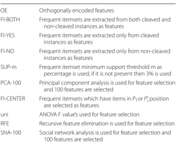
Table 1 Abbreviation and explanation
Abbreviation Explanation
OE Orthogonally encoded features
FI-BOTH Frequent itemsets are extracted from both cleaved and non-cleaved instances as features
FI-YES Frequent itemsets are extracted only from cleaved instances as features
FI-NO Frequent itemsets are extracted only from non-cleaved instances as features
SUP-m Frequent itemset minimum support threshold m as percentage is used; if it is not present then 3% is used PCA-100 Principal component analysis is used for feature selection
and 100 features are selected
FI-CENTER Frequent itemsets which have items in P1 or P′1 position
are selected as features
uni ANOVA F value’s used for feature selection
RFE Recursive feature elimination is used for feature selection SNA-100 Social network analysis is used for feature selection and
100 features are selected
Table 2 746 Dataset—without feature selection
Significant values are typed in italic
Methodology Accuracy Precision Recall F1 ROC-AUC
OE 0.869 0.871 0.910 0.883 0.956 FI-BOTH 0.869 0.904 0.860 0.869 0.956 OE + FI-BOTH 0.863 0.888 0.870 0.869 0.955 FI-YES 0.887 0.905 0.897 0.896 0.962 OE + FI-YES 0.871 0.891 0.882 0.878 0.958 FI-NO 0.873 0.904 0.877 0.880 0.949 OE + FI-NO 0.883 0.893 0.905 0.893 0.953 CMAR 0.789 0.812 0.79 0.783 0.777 CPAR 0.662 0.712 0.854 0.777 NA
are added into frequent itemset features and the perfor-mance of this dataset is measured.
The first thing we noticed is that PCA selection reduces accuracy when only orthogonal encoding is used. Com-pared to orthogonal encoding, selecting frequent item-sets on cleaved instances (FI-YES) yield better results in terms of accuracy, f1 and ROC-AUC scores. FI-BOTH performed similar compared to OE. Among these three, FI-NO has the worst accuracy.
Combining orthogonal encoding features and frequent itemset features reported some interesting results. For FI-YES, this combination yields worse f1 score compared to using only FI-YES. For FI-BOTH, combining it with OE has no effect on f1 score. This can be explained as fre-quent itemsets derived from FI-YES and FI-BOTH can represent the dataset with similar degree compared to OE. For this reason, adding OE and FI-YES or FI-BOTH gives us worse or similar results by increasing dimension-ality without adding much information. But, combin-ing OE and FI-NO improves f1 score compared to uscombin-ing FI-NO only.
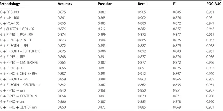
Table 3 shows the results of using feature selection. Among all features, 100 features are selected before testing the classifier using PCA, uni and RFE. It is important to note that all combinations of FI and OE with PCA yield better results compared to OE and PCA only. Lastly, best result of this experiment is achieved by combining OE, FI-NO and RFE-100. This score is also better than FI-BOTH and OE + FI-BOTH reported in Table 2.
Impens dataset
Results for this dataset are reported in Tables 4 and 5, without and with feature selection. Compared to the base case, FI-BOTH and FI-NO have better accuracy but worse f1 score in Table 4. FI-YES has worst f1 score among all fre-quent itemset methods and CPAR has the worst f1 score of all experiments. In this dataset, using OE with frequent itemset methods improves f1 scores. In our experiments, using OE with FI-BOTH yields the best results among FI based methods and CMAR has the best results among all for Impens dataset without feature selection.
In feature selection case, experiments with frequent itemsets have higher accuracy compared to without fea-ture selection counterpart. Also it is interesting to see that using FI-CENTER and selecting itemsets which have
Table 3 746 Dataset—with feature selection
Significant values are typed in italic
Methodology Accuracy Precision Recall F1 ROC-AUC
OE + RFE-100 0.875 0.882 0.905 0.885 0.961 OE + UNI-100 0.861 0.865 0.902 0.876 0.95 OE + PCA-100 0.865 0.883 0.880 0.872 0.949 OE + FI-BOTH + PCA-100 0.876 0.912 0.862 0.877 0.962 OE + FI-YES + PCA-100 0.874 0.899 0.872 0.877 0.961 OE + FI-NO + PCA-100 0.873 0.904 0.865 0.875 0.957 OE + FI-BOTH + RFE 0.872 0.893 0.887 0.879 0.958
OE + FI-BOTH +CENTER RFE 0.875 0.888 0.892 0.883 0.957
OE + FI-YES + RFE 0.868 0.89 0.877 0.874 0.956
OE + FI-YES + CENTER RFE 0.865 0.887 0.877 0.872 0.956
OE + FI-NO + RFE 0.866 0.88 0.89 0.875 0.953
OE + FI-NO + CENTER RFE 0.887 0.893 0.912 0.897 0.960
OE + FI-BOTH + uni 0.859 0.888 0.863 0.866 0.935
OE + FI-BOTH + CENTER uni 0.842 0.867 0.862 0.855 0.934
OE + FI-YES + uni 0.840 0.868 0.850 0.851 0.927
OE + FI-YES + CENTER uni 0.864 0.893 0.870 0.871 0.938
OE + FI-NO + uni 0.866 0.887 0.885 0.878 0.950
OE + FI-NO + CENTER uni 0.860 0.872 0.885 0.869 0.951
Table 4 Impens dataset—without feature selection
Significant values are typed in italic
Methodology Accuracy Precision Recall F1 ROC-AUC
OE 0.876 0.620 0.645 0.636 0.899 FI-BOTH 0.889 0.675 0.603 0.628 0.893 OE + FI-BOTH 0.885 0.654 0.696 0.659 0.903 FI-YES 0.866 0.609 0.656 0.609 0.890 OE + FI-YES 0.871 0.622 0.649 0.615 0.906 FI-NO 0.882 0.634 0.569 0.590 0.880 OE + FI-NO 0.879 0.625 0.67 0.634 0.900 CMAR 0.842 0.71 0.843 0.771 0.5 CPAR 0.552 0.277 0.83 0.416 NA
a P1 or P1′ position item, always increase accuracy and ROC-AUC score. Also F1 score increased for FI-YES and FI-NO. Biggest improvement happens with FI-NO and the best result among all feature selection experiments is using OE with FI-BOTH and filtering by FI-CENTER selected by RFE. This case also has better performance than the OE base case.
1625 dataset
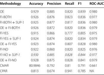
Results for this dataset are given in Tables 6 and 7. For without feature selection case, using only frequent item-sets based methods performed worse compared to base case in terms of f1 score and accuracy. Combining OE and frequent itemsets based methods improved per-formance for FI-YES and FI-NO. We also tried chang-ing minimum support threshold to observe the change in accuracy and f1 score. Minimum support thresh-old for choosing maximal frequent itemsets have been changed from 3 to 1%. For FI-YES and FI-NO this change improved performance significantly and FI-NO with SUP-1 is our best result among all.
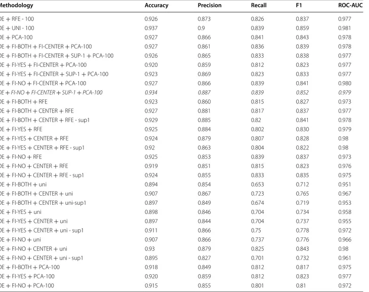
For feature selection case, FI-CENTER is applied to the combination of OE and frequent itemsets based meth-ods. With only this addition, it couldn’t perform better than base case. After realizing the positive outcome of changing minimum support threshold, it was decreased
to 1 percent. This change increased performance for FI-YES and FI-NO and most notable change happened for FI-NO. By applying this change, better results than base case were reported.
Schilling dataset
Results for this dataset are reported in Tables 8 and 9. For this dataset, FI-NO performed better than FI-YES, but the best performing method is FI-BOTH among FI
Table 5 Impens dataset—with feature selection
Significant values are typed in italic
Methodology Accuracy Precision Recall F1 Roc-Auc
OE + RFE 100 0.89 0.676 0.662 0.652 0.901
OE + UNI 100 0.881 0.662 0.616 0.625 0.901
OE + PCA-100 0.871 0.620 0.623 0.662 0.889
OE + FI-BOTH + PCA-100 0.891 0.672 0.596 0.627 0.893
OE + FI-BOTH + FI-CENTER + PCA-100 0.893 0.706 0.576 0.621 0.897
OE + FI-YES + PCA-100 0.881 0.650 0.596 0.611 0.886
OE + FI-YES + FI-CENTER + PCA-100 0.888 0.669 0.602 0.622 0.890
OE + FI-NO + PCA-100 0.879 0.640 0.570 0.593 0.880
OE + FI-NO + FI-CENTER + PCA-100 0.895 0.685 0.630 0.650 0.901
OE + FI-BOTH + RFE 0.886 0.663 0.61 0.625 0.890
OE + FI-BOTH + FI-CENTER + RFE 0.896 0.678 0.675 0.666 0.911
OE + FI-YES + RFE 0.880 0.661 0.662 0.641 0.910
OE + FI-YES + FI-CENTER + RFE 0.891 0.670 0.669 0.655 0.910
OE + FI-NO + RFE 0.879 0.634 0.649 0.631 0.892
OE + FI-NO + FI-CENTER + RFE 0.889 0.675 0.622 0.635 0.902
OE + FI-BOTH + uni 0.889 0.712 0.590 0.639 0.896
OE + FI-BOTH + FI-CENTER + uni 0.879 0.666 0.589 0.612 0.891
OE + FI-YES + uni 0.862 0.656 0.603 0.603 0.871
OE + FI-YES + FI-CENTER + uni 0.886 0.679 0.610 0.637 0.899
OE + FI-NO + uni 0.889 0.698 0.610 0.645 0.893
OE + FI-NO + FI-CENTER + uni 0.882 0.668 0.596 0.619 0.888
Table 6 1625 Dataset—without feature selection
Methodology Accuracy Precision Recall F1 ROC-AUC
OE 0.929 0.885 0.820 0.839 0.980 FI-BOTH 0.926 0.876 0.823 0.836 0.977 FI-BOTH + SUP-1 0.925 0.877 0.817 0.836 0.980 OE + FI-BOTH 0.926 0.872 0.820 0.836 0.979 FI-YES 0.915 0.866 0.777 0.805 0.975 FI-YES + SUP-1 0.924 0.874 0.820 0.834 0.979 OE + FI-YES 0.923 0.874 0.807 0.828 0.980 FI-NO 0.922 0.860 0.820 0.825 0.976 FI-NO + SUP-1 0.930 0.885 0.828 0.844 0.977 OE + FI-NO 0.928 0.875 0.828 0.841 0.979 CMAR 80.9846 0.792 0.81 0.791 0.661 CPAR 0.813 0.674 0.941 0.785 NA
methods. Also FI-BOTH performed better than base case and overall CMAR has the highest f1 score.
For feature selection case, all frequent itemsets com-bined methods performed better when compared to FI
only counterpart. Among them, combining OE with FI-YES and filtering by FI-CENTER performed the best as demonstrated by the reported results.
Characteristics of patterns sfter RFE ranking
We have performed experiments for ranking features with RFE. We have applied three different approaches. The first approach considers adopting both cleavage and non-cleavage training data for frequent itemset genera-tion, the second approach considers only cleaving train-ing data for frequent itemset generation, and the last approach considers only non-cleaving training data. The results are summarized in Tables 10, 11, and 12
We have composed top ten features for the datasets after RFE ranking of OE FI-BOTH in Table 10. The
Table 7 1625 Dataset—with feature selection
Significant values are typed in italic
Methodology Accuracy Precision Recall F1 ROC-AUC
OE + RFE - 100 0.926 0.873 0.826 0.837 0.977
OE + UNI - 100 0.937 0.9 0.839 0.859 0.981
OE + PCA-100 0.927 0.866 0.841 0.843 0.978
OE + FI-BOTH + FI-CENTER + PCA-100 0.927 0.861 0.836 0.839 0.978
OE + FI-BOTH + FI-CENTER + SUP-1 + PCA-100 0.926 0.865 0.833 0.838 0.977
OE + FI-YES + FI-CENTER + PCA-100 0.920 0.859 0.812 0.823 0.977
OE + FI-YES + FI-CENTER + SUP-1 + PCA-100 0.923 0.869 0.823 0.833 0.977
OE + FI-NO + FI-CENTER + PCA-100 0.927 0.866 0.839 0.841 0.980
OE + FI-NO + FI-CENTER + SUP-1 + PCA-100 0.934 0.887 0.839 0.852 0.979
OE + FI-BOTH + RFE 0.923 0.860 0.815 0.827 0.973
OE + FI-BOTH + CENTER + RFE 0.927 0.881 0.817 0.837 0.977
OE + FI-BOTH + CENTER + RFE - sup1 0.929 0.885 0.82 0.841 0.978
OE + FI-YES + RFE 0.925 0.884 0.802 0.830 0.979
OE + FI-YES + CENTER + RFE 0.924 0.879 0.807 0.828 0.98
OE + FI-YES + CENTER + RFE - sup1 0.92 0.863 0.804 0.822 0.98
OE + FI-NO + RFE 0.925 0.853 0.839 0.837 0.973
OE + FI-NO + CENTER + RFE 0.919 0.851 0.815 0.823 0.976
OE + FI-NO + CENTER + RFE - sup1 0.924 0.855 0.833 0.835 0.975
OE + FI-BOTH + uni 0.894 0.854 0.653 0.712 0.951
OE + FI-BOTH + CENTER + uni 0.907 0.867 0.723 0.765 0.967
OE + FI-BOTH + CENTER + uni-sup1 0.897 0.849 0.674 0.719 0.953
OE + FI-YES + uni 0.898 0.846 0.704 0.734 0.958
OE + FI-YES + CENTER + uni 0.897 0.844 0.704 0.737 0.955
OE + FI-YES + CENTER + uni - sup1 0.911 0.866 0.75 0.778 0.972
OE + FI-NO + uni 0.907 0.866 0.737 0.776 0.966
OE + FI-NO + CENTER + uni 0.93 0.879 0.825 0.843 0.98
OE + FI-NO + CENTER + uni - sup1 0.895 0.827 0.701 0.732 0.961
OE + FI-BOTH + PCA-100 0.918 0.849 0.812 0.817 0.975
OE + FI-YES + PCA-100 0.920 0.859 0.812 0.823 0.977
OE + FI-NO + PCA-100 0.915 0.855 0.801 0.81 0.972
Table 8 Schilling dataset—without feature selection
Significant values are typed in italic
Methodology Accuracy Precision Recall F1 ROC-AUC
OE 0.907 0.706 0.683 0.661 0.941 FI-BOTH 0.922 0.774 0.623 0.668 0.949 FI-YES 0.904 0.714 0.653 0.645 0.938 FI-NO 0.918 0.754 0.607 0.650 0.949 CMAR 0.867 0.752 0.867 0.806 0.5 CPAR 0.488 0.189 0.857 0.310 NA
results indicate that for 746 dataset, nine out of ten are mostly observed as majority for cleavage instances. For 1625 dataset, six of them are cleavage and three of them
are non-cleavage instances; one pattern is equally dis-tributed between both. For impens and schilling data-sets, 1-item frequent items are ranked in the first ten
Table 9 Schilling dataset—with feature selection
Significant values are typed in italic
Methodology Accuracy Precision Recall F1 ROC-AUC
OE + RFE 100 0.911 0.71 0.702 0.675 0.943
OE + UNI 100 0.911 0.697 0.69 0.673 0.939
OE + PCA-100 0.886 0.581 0.631 0.614 0.920
OE + FI-BOTH + FI-CENTER + PCA-100 0.926 0.765 0.663 0.699 0.941
OE + FI-YES + FI-CENTER + PCA-100 0.931 0.797 0.665 0.715 0.951
OE + FI-NO + FI-CENTER + PCA-100 0.927 0.777 0.667 0.701 0.945
OE + FI-BOTH + RFE 0.911 0.718 0.667 0.66 0.941
OE + FI-BOTH + FI-CENTER + RFE 0.912 0.719 0.692 0.672 0.948
OE + FI-YES + RFE 0.909 0.703 0.695 0.674 0.944
OE + FI-YES + FI-CENTER + RFE 0.911 0.695 0.697 0.679 0.942
OE + FI-NO + RFE 0.913 0.72 0.676 0.668 0.939
OE + FI-NO + FI-CENTER + RFE 0.911 0.712 0.681 0.667 0.945
OE + FI-BOTH + uni 0.9 0.655 0.619 0.612 0.924
OE + FI-BOTH + FI-CENTER + uni 0.908 0.679 0.692 0.668 0.936
OE + FI-YES + uni 0.876 0.605 0.579 0.56 0.896
OE + FI-YES + FI-CENTER + uni 0.892 0.639 0.618 0.605 0.913
OE + FI-NO + uni 0.93 0.879 0.825 0.843 0.98
OE + FI-NO + FI-CENTER + uni 0.909 0.686 0.697 0.672 0.937
OE + FI-BOTH 0.908 0.706 0.683 0.66 0.94 OE + FI-NO 0.907 0.707 0.676 0.655 0.94 OE + FI-YES 0.9 0.712 0.706 0.677 0.941 OE + FI-BOTH + PCA-100 0.926 0.765 0.663 0.699 0.941 OE + FI-YES + PCA-100 0.931 0.797 0.665 0.715 0.951 OE + FI-NO + PCA-100 0.911 0.728 0.547 0.6 0.917
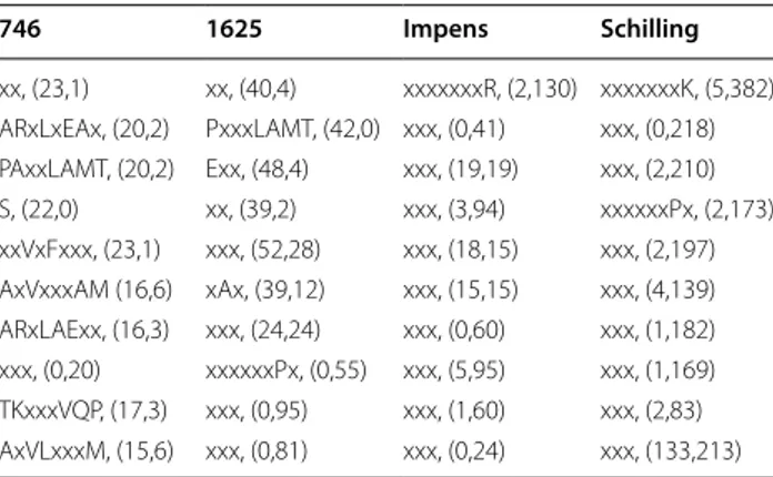
Table 10 Top ten patterns obtained with OE including fre-quent itemsets after RFE (FI-BOTH RFE) with (cleavage, non-cleavage) distribution 746 1625 Impens Schilling xx, (23,1) xx, (40,4) xxxxxxxR, (2,130) xxxxxxxK, (5,382) ARxLxEAx, (20,2) PxxxLAMT, (42,0) xxx, (0,41) xxx, (0,218) PAxxLAMT, (20,2) Exx, (48,4) xxx, (19,19) xxx, (2,210) S, (22,0) xx, (39,2) xxx, (3,94) xxxxxxPx, (2,173) xxVxFxxx, (23,1) xxx, (52,28) xxx, (18,15) xxx, (2,197) AxVxxxAM (16,6) xAx, (39,12) xxx, (15,15) xxx, (4,139) ARxLAExx, (16,3) xxx, (24,24) xxx, (0,60) xxx, (1,182) xxx, (0,20) xxxxxxPx, (0,55) xxx, (5,95) xxx, (1,169) TKxxxVQP, (17,3) xxx, (0,95) xxx, (1,60) xxx, (2,83) AxVLxxxM, (15,6) xxx, (0,81) xxx, (0,24) xxx, (133,213)
Table 11 Top ten patterns obtained with OE including fre-quent itemsets after RFE (FI-YES RFE) with (cleavage, non-cleavage) distribution
746 1625 Impens Schilling
xxxFxExx (12,0) PxVSLAMT (10,0) xEx (4,20) xx (15,2) SQxYYxxx (11,0) SQxYYxxx (11,0) xExRxxxx (4,0) xFx (14,5) PxVxLAMT (27,0) AxVLAEAx (13,0) xx (4,0) Exx (16,14) xKxLVVQP (14,1) TxxLVVQP (14,1) xxIxYxxx (4,1) xx (13,1) x (14,0) xx (11,1) xxxxxEYx (4,0) xx (13,21) Exx (13,0) PxxWLAMT (10,0) xx (4,0) Ixx (12,15) xxNxPQxx (12,0) SxTYYxDS (11,0) xx (4,1) xxxxIxLx (12,4) SDTYYxxS (11,0) xGx (10,0) xx (6,3) Pxx (12,8) xQNYPIVQ (11,0) SxxYYTDS (11,0) xxxLxLxx (5,2) xFExxxxx (13,3) SxNxPxVQ (11,3) SGxxxxxS (11,1) xWxxxxxx (4,0) xxx (36,37)
where percentage of cleavage dataset is higher for one of them; equal for cleavage and non-cleavage. Remain-ing eight patterns are mostly observed for non-cleavage datasets. For schilling dataset, all are mostly seen in non-cleavage data. Impens and schilling patterns are located close to center. It would be reasonable to pay attention to non-cleavage patterns mostly for development of inhibitors.
In Table 11, frequent itemsets obtained from cleaved training data have been used for feature ranking and top ten patterns have been presented for the datasets. Major-ity of patterns are attributed to cleaving data in the entire dataset. Itemsets that contain six or 7 items are ranked in the first ten patterns. They are not listed in FI-BOTH experiment. Itemsets containing more than one item occur in Impens and Schilling datasets. Nine of them occur more in cleaving instances and one in non-cleaving instances. It may be surprising that one pattern obtained in FI-YES may exist in non-cleaving instances but occur-rence of same pattern in non-cleaving instances is pos-sible. This is similar for Schilling dataset. Eight patterns exist mostly in cleaving instances and two exist in non-cleaving instances. Patterns represent instances having significant positions closer to center.
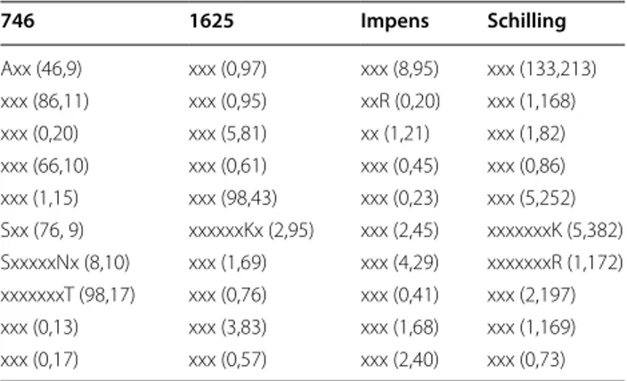
In Table 11, non-cleaved instances have been mined to extract frequent patterns from non-cleaving instances(FI-NO). Top ten patterns have been listed for the datasets. It is noticeable that patterns are mostly 1-item frequent itemsets. The reason is that we were unable to find char-acteristic patterns for non-cleavage since they are col-lected from dispersed space. For 746 dataset, 5 cleavage and 5 non-cleavage; for 1625 dataset, one cleavage and nine non-cleavage and for Impens and Schilling datasets; all patterns are mostly found in non-cleavage instances. Again, patterns closer to center are identified as signifi-cantly top ranking patterns.
Complementary analysis by social network analysis
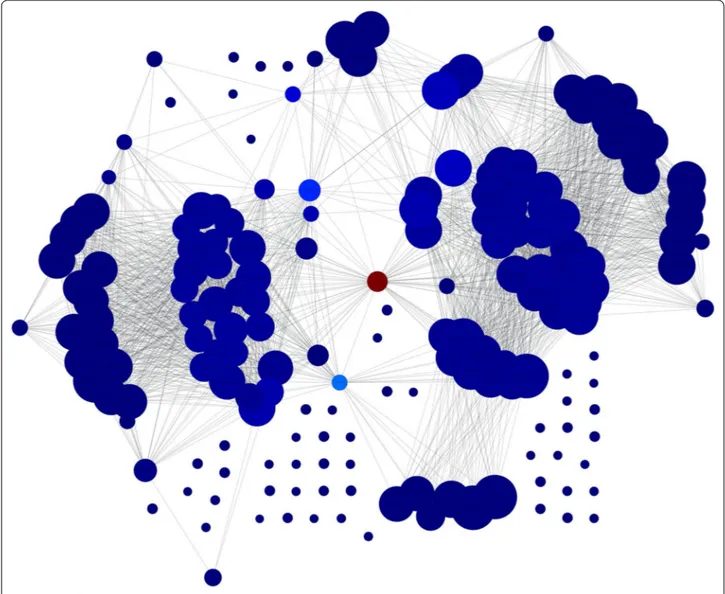
For the network created based on frequent itemsets, PageRank and betweenness centrality measures are computed and the top 50 frequent itemsets are chosen. Histograms are created to understand the distribution of the selected features. Histograms of each item are shown in Figs. 1 and 2, for pagerank and betweenness, respec-tively. Figure 3 visualizes the network where color has been determined according to pagerank centrality values using jet colormap. Figue 4 displays the network where color has been determined according to betweenness centrality values using jet colormap. Finally, top five fea-tures are reported in Tables 13 and 14 for pagerank and betweenness, respectively.
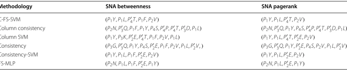
The selected features are compared with the results reported in [14]. Authors of [14] have worked with 754 dataset; for this reason, we compared our findings from 746 dataset. Intersection of selected features and inter-section amount are presented in Tables 15 and 16.
Comparison of algorithms without feature selection
We have used Keel application [27] to estimate effective-ness of our algorithm.6 Average ranks have been obtained by applying Friedman procedure.
Table 17 summarizes the f-score ranking of algorithms having no feature selection. Ranking has been computed with Friedman statistic with (9 − 1) degrees of freedom and distribution of chi-square as 7.2. P value computed by Friedman test was 0.515.
Based on the results, recommended orthogonal encoding scheme with SVM classifier performs the best [13]. Overall analysis of algorithms indicate that OE with SVM performs the best with overall ranking result value 3.25. OE + FI-NO ranks second algorithm with overall ranking result value, which is 3.5. Next two algo-rithms OE + FI-BOTH and CMAR get the third place with value as 4.5. FI-BOTH value is 4.75. OE + FI-YES is 5, and FI-YES value is 6. CPAR has the worst rank-ing overall. Accordrank-ing to the null hypothesis, all classifi-ers have no difference; this is rejected since they are not equal.
Later, We have performed N ∗ N post hoc compari-son with Shaffer’s statistical test. Additional file 1: Table S1 gives comparison results between algorithms. In this table, p and adjusted Shaffer p value as the adjusted value are listed. Comparison results give p values which when higher favor the null hypothesis that claims that the compared two algorithms are not significantly different.
6 http://www.keel.es/algorithms.php. Table 12 Top ten patterns obtained with OE
including fre-quent itemsets after RFE (FI-NO RFE) with (cleavage, non-cleavage) distribution 746 1625 Impens Schilling Axx (46,9) xxx (0,97) xxx (8,95) xxx (133,213) xxx (86,11) xxx (0,95) xxR (0,20) xxx (1,168) xxx (0,20) xxx (5,81) xx (1,21) xxx (1,82) xxx (66,10) xxx (0,61) xxx (0,45) xxx (0,86) xxx (1,15) xxx (98,43) xxx (0,23) xxx (5,252) Sxx (76, 9) xxxxxxKx (2,95) xxx (2,45) xxxxxxxK (5,382) SxxxxxNx (8,10) xxx (1,69) xxx (4,29) xxxxxxxR (1,172) xxxxxxxT (98,17) xxx (0,76) xxx (0,41) xxx (2,197) xxx (0,13) xxx (3,83) xxx (1,68) xxx (1,169) xxx (0,17) xxx (0,57) xxx (2,40) xxx (0,73)
We repeated the statistical analysis for algorithms with feature selection including OE with SVM and the first one bundled with feature selection algorithms such as RFE and univariate Anova analysis. Table 18 summarizes the f-score ranking of algorithms having no feature selec-tion. Ranking has been computed with Friedman sta-tistic with (22 − 1) degrees of freedom and distribution
of chi-square as 39.139328. P-value computed by Fried-man test was 0.009445911037720411. Based on the results, ranking of the listed algorithms are different and OE + FI-NO + FI-CENTER + PCA-100 outperforms OE and OE + RFE. Its ranking value is 3.375. The second ranked algorithms are OE FI-BOTH CENTER RFE and OE + RFE(6). OE has the value 9.125.
Fig. 1 Histogram for 50 features selected by PageRank centrality
Later, we performed N ∗ N post hoc comparison with Shaffer’s statistical test. Additional file 1: Table S2 gives comparison results between algorithms. This table lists p and adjusted Shaffer p value as the adjusted value. Com-parison results give p values which when higher favor the null hypothesis that claims that the compared two algo-rithms are not significantly different.
Conclusions and future work
AIDS is a deadly disease caused by HIV. Cleaving pro-teins is an important event for HIV. Understanding patterns for this process will lead to improvements on drug design. The proposed approach views HIV data from a different perspective, where features are Fig. 3 Graph for network colored by PageRank
enriched with frequent itemsets, with support values with respect to their occurrences within the training data. Hence, features are reorganized at each section
in cross validation. This is a novel approach in terms of feature extraction and dimensionality reduction. Our approach to tackle this problem was to extract frequent itemsets based on sequential amino acids in octomer. Three different sets of maximal frequent itemsets are extracted based on cleave property of an instance. These maximal frequent itemsets are used as features and the intersection of instance and feature are filled according to similarity function. After this process, a dataset is fit into the machine learning algorithm and results are reported.
Our results show that using frequent itemsets as fea-tures has positive impact on performance. For some cases, using only frequent itemsets as features can Fig. 4 Graph for network colored by betweenness
Table 13 Top 5 vertices according to PageRank
Vertex Centrality score
(P3G, P4S, P2V ) 0.0088053091045 (P4′P, P3′Q, P1L, P2V , P′2V ) 0.00729830131176 (P′ 4M, P3′A, P4A, P1L, P2V ) 0.00726810634265 (P′ 1A, P′3A, P4A, P1L, P2V ) 0.00726810634265 (P3R, P3′A, P4A, P1L, P2V ) 0.00726810634265
represent a dataset better than OE. For other cases, frequent itemsets features can be used as supplemen-tary features which also improved performance com-pared to OE. In most cases, feature selection among the combination of OE and FI-based methods yields bet-ter performance and using less features compared to OE. Minimum support threshold is also an important parameter for FI-based methods, changing it can lead to increased performance.
Our complementary analysis benefits from itemsets to generate a network which will help in finding impor-tant features by using SNA metrics described in the lit-erature. In general, they are used to understand dynamics of social networks. Particularly, in our work, it is used to understand the relationship between residues and amino acid groups. For top 50 features, histograms of items are presented. Top 5 features are reported and graph is visualized to see the influence between features. Also the chosen features are compared with another work and similarities between selected features are shown. All
Table 14 Top 5 vertices according to betweenness
Vertex Centrality score
(P3G, P4S, P2V ) 0.152425782917 (P′ 4T , P4S) 0.0356197541186 (P3G, P′2V , P4S) 0.0254409174283 (P1F, P2′V ) 0.0119543726703 (P′ 4P, P3′Q, P1L, P2V , P′2V ) 0.00917331679147
Table 15 Intersection between selected features
Methodology SNA betweenness SNA pagerank
C-FS-SVM 5 4 Column Ccnsistency 9 8 Column SVM 7 5 Consistency 9 8 Consistency-SVM 5 4 FS-MLP 5 4
Table 16 Intersected features between selected features
Methodology SNA betweenness SNA pagerank
C-FS-SVM (P1Y , P1L, P4′T , P1F, P2V ) (P1Y , P1L, P4′T , P2V ) Column consistency (P2N, P3′Q, P1F, P1Y , P4S, P′4P, P4′T , P3′D, P1L) (P2N, P3′Q, P1Y , P4S, P′4P, P′4T , P′3D, P1L) Column SVM (P1Y , P3K , P2′E, P′4T , P1F, P2V , P1L) (P1Y , P1L, P4′T , P2′E, P2V ) Consistency (P3G, P′3Q, P1Y , P4S, P′2E, P1F, P2V , P1L, P2′V , ) (P3G, P′3Q, P1Y , P2′E, P4S, P2V , P1L, P′2V ) Consistency-SVM (P1Y , P1L, P1F, P′2E, P2V ) (P1Y , P1L, P2′E, P2V ) FS-MLP (P2N, P1L, P1F, P2′E, P1Y ) (P2N, P1L, P2′E, P1Y )
Table 17 Average ranking of the algorithms without fea-ture selection Algorithm Ranking OE 3.25 FI-BOTH 4.75 OE + FI-BOTH 4.5 FI-YES 6 OE + FI-YES 5 FI-NO 6.25 OE + FI-NO 3.5 CMAR 4.5 CPAR 7.25
Table 18 Average rankings of the algorithms
Algorithm Ranking
OE 9.125
OE + PCA-100 10.125
OE + FI-BOTH + PCA-100 10.75
OE + FI-BOTH + FI-CENTER + PCA-100 9.375
OE + FI-YES + PCA-100 11
OE + FI-YES + FI-CENTER + PCA-100 9
OE + FI-NO + PCA-100 18.125
OE + FI-NO + FI-CENTER + PCA-100 3.375
OE FI-BOTH RFE 12.25
OE FI-BOTH CENTER RFE 6
OE FI-YES RFE 10
OE FI-YES CENTER RFE 9
OE FI-NO RFE 11.375
OE FI-NO CENTER RFE 10
OE FI-BOTH uni 17.25
OE FI-BOTH CENTER uni 18
OE FI-YES uni 21.5
OE FI-YES CENTER uni 17
OE FI-NO uni 12.25
OE FI-NO CENTER uni 12.25
OE+RFE 6
these results demonstrate effectiveness of the proposed methodology.
In-depth analysis for making biological explanation remains another future direction. In the future, fascicles of different domains on molecular biology will be studied.
Authors’ contributions
The three authors contributed to the manuscript writing, editing and finalizing. The three authors also contributed to the development of the methodology. In particular, YK wrote the software and run the testing, TO closely mentored the study and RA edited the final draft and made it ready for submission. All authors read and approved the final manuscript.
Author details
1 Department of Computer Engineering, TOBB University, Ankara, Turkey. 2 Department of Computer Science, University of Calgary, Calgary, Canada. Acknowledgements
We would like to thank reviewers and editor handling our submission for their time and effort. The software is available and can be downloaded from: http:// tinyurl.com/hf77gvg.
Competing interests
The authors declare that they have no competing interests. Received: 19 March 2016 Accepted: 20 November 2016
References
1. Global Health Observatory (GHO) data. http://www.who.int/gho/hiv/en/. Accessed 19 Feb 2016
2. Grossman CI, Ross AL, Auerbach JD, Ananworanich J, Dubi K, Tucker JD, Noseda V, Possas C, Rausch DM (2016) Towards Multidisciplinary HIV-Cure Research: Integrating Social Science with Biomedical Research. Trends Microbiol 24(1):5–11
3. De Clercq E (2004) Antiviral drugs in current clinical use. J Clin Virol 30:115–133
4. Rögnvaldsson T, You L, Garwicz D (2007) Bioinformatic approaches for modeling the substrate specificity of HIV-1 protease: an overview. Expert Rev Mol Diagn 7(4):435–451
5. Gök M, Özcerit AT (2013) A new feature encoding scheme for HIV-1 pro-tease cleavage site prediction. Neural Comput Appl 22(7–8):1757–1761 6. Nanni L, Lumini A (2009) Using ensemble of classifiers for predicting HIV
protease cleavage sites in proteins. Amino Acids 36(3):409–416 7. Thompson TB, Chou KC, Zheng C (1995) Neural network prediction of the
HIV-1 protease cleavage sites. J Theor Biol 177(4):369–379 8. Cai YD, Liu XJ, Xu XB, Chou KC (2002) Support vector machines for
predicting HIV protease cleavage sites in protein. J Comput Chemstry 23(2):267–274
9. Rama GLJ, Palaniswami M (2005) Cleavage knowledge extraction in HIV-1 protease using hidden Markov model. In: Proceedings of 2005 interna-tional conference on intelligent sensing and information processing, 2005. IEEE, pp 469–473
10. Agrawal R, Srikant R (1994) Fast algorithms for mining association rules. Proc Int Conf Very Large Databases 1215:487–499
11. Heikki M, Toivonen H (1997) Levelwise search and borders of theories in knowledge discovery. Data Min Knowl Discov 1(3):241–258
Additional file
Additional file 1. Non-parametric statistic methods for comparative analysis between methods.
12. Pasquier N, Bastide Y, Taouil R, Lakhal L (1999) Discovering frequent closed itemsets for association rules. Database theory-ICDT-99. Springer, New York, pp 398–416
13. Rögnvaldsson T, You L, Garwicz D (2015) State of the art prediction of HIV-1 protease cleavage sites. Bioinformatics 31(8):1204–1210 14. Öztürk O, Aksaç A, Elsheikh A, Özyer T, Alhajj R (2013) A
consistency-based feature selection method allied with linear SVMs for HIV-1 protease cleavage site prediction. PLoS One 8(8):e63145
15. You L, Daniel Garwicz D (2005) Rögnvaldsson thorsteinn comprehen-sive bioinformatic analysis of the specificity of human immunode-ficiency virus type 1 protease. J Virol 79:12477–12486. doi:10.1128/ jvi.79.19.12477-12486
16. Kontijevskis A, Prusis P, Petrovska R, Yahorava S, Mutulis F, Mutule I, Komorowski J, Wikberg JES (2007) A look inside HIV resistance through retroviral protease interaction maps. PLoS Comput Biol 3(3):e48 17. Schilling O, Overall CM (2008) Proteome-derived, database-searchable
peptide libraries for identifying protease cleavage sites. Nat Biotechnol 26(6):685–694
18. Borgelt C (2005) An implementation of the FP-growth algorithm. In: Pro-ceedings of the 1st international workshop on open source data mining: frequent pattern mining implementations. ACM, pp 1–5
19. Han J, Pei J, Yin Y (2000) Mining frequent patterns without candidate generation. In: ACM sigmod record, vol 29, 2nd edn. ACM, pp 1–12 20. Kontijevskis A (2007) Computational proteomics analysis of HIV-1
pro-tease interactome. Proteins 68:305–312
21. Impens F et al (2012) A catalogue of putative HIV-1 protease host cell substrates. Biol Chem 393:915–931
22. Alvarez E et al (2006) HIV protease cleaves poly(A)-binding protein. Biochem J 396:219–226
23. Gerencer M, Burek V (2004) Identification of HIV-1 protease cleavage site in human C1-inhibitor. Virus Res 105:97–100
24. Nie Z et al (2007) Human immunodeficiency virus type 1 protease cleaves procaspase 8 in vivo. J Virol 81:6947–6956
25. Li W, Han J, Pei J (2001) CMAR: accurate and efficient classification based on multiple class-association rules. In: Proceedings IEEE international conference on data mining, 2001. ICDM 2001. IEEE
26. Yin X, Han J (2003) CPAR classification based on predictive association rules. Proc SDM
27. Alcalá-Fdez J et al (2009) KEEL: a software tool to assess evolutionary algorithms for data mining problems. Soft Comput 13.3:307–318 28. Page L, Brin S, Motwani R, Winograd T (1999) The pagerank citation
rank-ing: bringing order to the web. Stanford InfoLab
29. Liao WWP, Arthur JW (2011) Predicting peptide binding affinities to MHC molecules using a modified semi-empirical scoring function. PLoS ONE 6.9:e25055