KADİR HAS UNIVERSITY SCHOOL OF GRADUATE STUDIES PROGRAM OF INDUSTRIAL ENGINEERING
A BEHAVIORAL STUDY FOR EXAMINING
THE COMPLIANCE OF PRICING MODELS
IN REVENUE MANAGEMENT THEORY
WITH THE DECISIONS OF
HUMAN DECISION MAKERS
CÜNEYT ERKOL
MASTER OF SCIENCE THESIS
C üne yt Erkol Ma ster of Scie n ce The sis 20 20 S tudent’ s F ull Na me P h.D. (or M.S . or M.A .) The sis 20 11
3
A BEHAVIORAL STUDY FOR EXAMINING
THE COMPLIANCE OF PRICING MODELS
IN REVENUE MANAGEMENT THEORY
WITH THE DECISIONS OF HUMAN DECISION MAKERS
CÜNEYT ERKOL
MASTER OF SCIENCE THESIS
Submitted to the School of Graduate Studies of
Kadir Has University in partial fulfillment of the requirements for the degree of Master of Science in Industrial Engineering.
ISTANBUL, AUGUST, 2020 APPENDIX B
DECLARATION OF RESEARCH ETHICS / METHODS OF DISSEMINATION
I, Cüneyt Erkol, hereby declare that;
• this Master’s Thesis is my own original work and that due references have been appropriately provided on all supporting literature and resources;
• this Master’s Thesis contains no material that has been submitted or accepted for a degree or diploma in any other educational institution;
• I have followed Kadir Has University Academic Ethics Principles prepared in accordance with The Council of Higher Education’s Ethical Conduct Principles.
In addition, I understand that any false claim in respect of this work will result in disciplinary action in accordance with University regulations.
Furthermore, both printed and electronic copies of my work will be kept in Kadir Has Information Center under the following condition as indicated below:
The full content of my thesis/project will be accessible from everywhere by all means.
CÜNEYT ERKOL
__________________________ August 14, 2020
KADİR HAS UNIVERSITY SCHOOL OF GRADUATE STUDIES
ACCEPTANCE AND APPROVAL
This work entitled A BEHAVIORAL STUDY FOR EXAMINING THE
COMPLIANCE OF PRICING MODELS IN REVENUE MANAGEMENT THEORY WITH THE DECISIONS OF HUMAN DECISION MAKERS prepared by CÜNEYT ERKOL has been judged to be successful at the defense exam on August 14, 2020 and accepted by our jury as MASTER OF SCIENCE THESIS.
APPROVED BY:
Asst. Prof. Nur AYVAZ ÇAVDAROĞLU (Advisor)
(Kadir Has University) _______________
Asst. Prof. Esra AĞCA AKTUNÇ (Co-advisor)
(Kadir Has University) _______________
Assoc. Prof. Ahmet Deniz YÜCEKAYA
(Kadir Has University) _______________
Asst. Prof. Emre ÇELEBİ
(Kadir Has University) _______________
Asst. Prof. Mürüvvet İlknur BÜYÜKBOYACI HANAY
(Middle East Technical University) _______________
I certify that the above signatures belong to the faculty members named above.
_______________ Prof. ……….. Dean of School of Graduate Studies DATE OF APPROVAL: ... / ... / 2020
TABLE OF CONTENTS
ABSTRACT ... i ÖZET ... ii ACKNOWLEDGEMENTS ... iii LIST OF TABLES ... v LIST OF FIGURES ... vi 1. INTRODUCTION ... 1 2. LITERATURE REVIEW ... 3 2.1. Revenue Management ... 3 2.2. Pricing Models ... 32.3. Behavioral Operations Management ... 4
2.4. Cognitive Biases ... 6 2.4.1. Anchoring Effect ... 6 2.4.2. Bounded Rationality ... 6 2.4.3. Demand-Chasing Bias ... 7 2.4.4. Gambler’s Fallacy ... 7 3. THEORETICAL MODEL ... 8
3.1. Theoretical Model of Experiments 1 and 2 ... 8
3.2. Theoretical Model of Experiments 3 and 4 ... 10
4. EXPERIMENTAL SETUP ... 12
4.1. Theoretical Benchmarks of Experiments... 12
4.2. Profile of Experiment Subjects ... 14
4.3. Recruitment Process of Experiment Subjects ... 15
4.4. Organization of Experimental Sessions ... 15
4.5. Monetary Budget used for Experiments ... 17
4.6. Usage of Software for Data Collection ... 17
4.7. Statistical Methods Used for Data Analysis ... 18
4.7.1. The Two-Tailed Wilcoxon Signed Rank Test ... 18
4.7.2. The Wilcoxon Rank-Sum Test ... 19
ii
4.8. Sample Sizes of Experiments ... 19
5. EXPERIMENT RESULTS ... 21
5.1. Comparison of Experiment Results with Theoretical Benchmarks ... 21
5.1.1. “Static Competitor Price” Treatment ... 21
5.1.2. “Dynamic Competitor Price” Treatment ... 27
5.2. Effects of Personality Traits ... 33
5.2.1. Cognitive Reflection Test Scores ... 33
5.2.2. Maximizing Tendency Scores ... 36
5.2.3. Risk Attitude Scores ... 38
5.3. Individual Behavior Patterns ... 44
6. DISCUSSION ... 48
6.1. Comparing the potential and realized revenues ... 48
6.2. Summary of Hypotheses and Conclusions Reached ... 49
6.3. Main Findings of the Study ... 50
7. CONCLUSION ... 53
7.1. Suggestions for Future Research ... 53
REFERENCES ... 55
APPENDIX A Questionnaire for Cognitive Reflection Test (CRT), Maximizing Tendency (MT) and Risk Scores of Test Subjects ... 59
A.1 Questions for Cognitive Reflection Test (CRT) ... 59
A.2 Questions for Maximizing Tendency (MT) ... 60
A.3 Questions for Risk Scores ... 61
APPENDIX B Instructions given to subjects during the Experiments ... 62
B.1 Instructions given during Experiment 1 ... 62
B.2 Instructions given during Experiment 2 ... 65
B.3 Instructions given during Experiment 3 ... 68
i
A BEHAVIORAL STUDY FOR EXAMINING THE COMPLIANCE OF PRICING MODELS
IN REVENUE MANAGEMENT THEORY
WITH THE DECISIONS OF HUMAN DECISION MAKERS
ABSTRACT
This study involves four computer-based experiments based on different assumptions which are performed in a laboratory-setting. The behavior patterns of the subjects and the degree of deviation of these behaviors from optimal strategies are analyzed by various statistical methods. The common aim of the experiments examined in this thesis is to understand how successful Revenue Management theoretical models are in explaining real human behavior. In various cases, it has been possible to determine in which direction deviations from theoretical models occur and causes can be understood. In static competitor price treatment (in experiments 1 and 2), subjects exhibit a higher tendency to underprice. The “gambler’s fallacy” bias is the dominant behavioral pattern observed in dynamic price setting. Humans consistently make pricing decisions below theoretical optimum, and only a small minority of the subjects are able to make optimum pricing decisions, supporting the presence of bounded rationality. Higher cognitive reflection skills help perform decisions closer to optimal, although not significantly better. Maximizing tendency does not show significance in meeting neither the optimum price, nor the potential revenue. Higher risk appetite makes better decisions in a dynamic competitor price setting. Neither the impact of learning effect, nor the demand-chasing bias is prevalent in the findings. Anchoring on the competitor price is observable in dynamic price setting. The study is useful in revealing the human factor issues that companies aiming to increase their profitability should pay attention to. Furthermore, the study can also be helpful in determining information to be provided to decision makers by an effective decision support system, and it proposes recommendations regarding the measures companies can take to improve human decision makers’ decisions.
Keywords: Revenue Management, Behavioral Operations Management, Cognitive Reflection, Maximizing Tendency, Risk Appetite, Pricing
ii
GELİR YÖNETİMİ TEORİSİNDEKİ FİYATLANDIRMA MODELLERİNİN İNSAN KARAR VERİCİLERİN KARARLARIYLA UYUMUNU İNCELEMEK İÇİN
BİR DAVRANIŞSAL ÇALIŞMA
ÖZET
Bu çalışma, laboratuvar ortamında yapılan ve farklı varsayımlara dayanan dört bilgisayar tabanlı deney gerçekleştirmektedir. Deneklerin davranış kalıpları ve bu davranışların optimal stratejilerden sapma derecesi çeşitli istatistiksel yöntemlerle analiz edilmektedir. Bu tezde incelenen deneylerin ortak amacı, Gelir Yönetimi teorik modellerinin gerçek insan davranışlarını açıklamada ne kadar başarılı olduğunu anlamaktır. Teorik modellerden hangi yönde sapmaların meydana geldiğini ve nedenlerinin anlaşılabileceğini belirlemek mümkün olmuştur. Rakip fiyatının sabit olduğu düzenekte (deney 1 ve 2'de), denekler düşük fiyatlandırma eğilimi göstermişlerdir. "Kumarbazın yanılgısı", dinamik rakip fiyatı düzeneğinde gözlemlenen baskın davranış kalıbıdır. İnsan karar vericiler ısrarla teorik optimumun altında fiyatlandırma kararları almakta olup, deneklerin yalnızca küçük bir azınlığının optimum fiyatlandırma kararları verebilmesi, sınırlı rasyonalitenin varlığını desteklemektedir. Daha yüksek bilişsel yansıtma becerileri, önemli ölçüde daha iyi olmasa da, optimal olana yakın kararlar almaya yardımcı olmuştur. Ençoklama eğilimi yüksek karar vericiler, ne optimum fiyatı bulmakta ne de potansiyel gelire ulaşmakta yetkindir. Daha yüksek risk iştahı olan karar vericiler, dinamik rakip fiyatı düzeneğinde daha iyi kararlar verir. Bulgularda ne öğrenme etkisi, ne de talep peşinde koşma önyargısı yaygın görülmüştür. Dinamik fiyatlandırma düzeneğinde rakip fiyat üzerine çıpa etkisi gözlemlenmiştir. Çalışma, kârlılıklarını artırmayı hedefleyen firmaların dikkat etmesi gereken insan faktörü konularının ortaya çıkarılması açısından faydalıdır. Ayrıca çalışma, etkili bir karar destek sistemi tarafından karar vericilere sağlanacak bilgilerin belirlenmesinde yardımcı olabilir ve şirketlerin insan karar vericilerin kararlarını iyileştirmek için alabilecekleri önlemlere ilişkin öneriler sunar.
Anahtar Sözcükler: Gelir Yönetimi, Davranışsal İşlemler Yönetimi, Bilişsel Yansıma, Ençoklama Eğilimi, Risk İştahı, Fiyatlandırma
iii
ACKNOWLEDGEMENTS
I gratefully acknowledge the support of TÜBİTAK, the Scientific and Technological Research Council of Turkey (Project ID: 218K341).
iv
To my mother and father for encouraging me to pursue my academic goals further
v
LIST OF TABLES
Table 1 Summary of the Experimental Setup..………...12
Table 2 Theoretical benchmarks for Experiments 1 and 2..………...13
Table 3 Theoretical benchmarks for Experiments 3 and 4.………...13
Table 4 Sample sizes of the Experiments..………...………...…20
Table 5 Comparison results of experiment performance with the optimal thresholds in Experiments 1 and 2….………...……….…...22
Table 6 Individual level comparison of pricing decisions with the optimal in Experiments 1 and 2………...23
Table 7 Comparison results of experiment performance with the optimal thresholds in Experiments 3 and 4………...……….………...28
Table 8 Individual level comparison of pricing decisions with the optimal in Experiments 3 and 4………...29
Table 9 Questions for Cognitive Reflection Test (CRT)………34
Table 10 Questions for Maximizing Tendency (MT)………..………...36
Table 11 Questions for Risk Scores………38
Table 12 Cumulative survey scores of subjects and their relative classes in CRT, MT and Risk Appetite …...………...41
Table 13 Comparison results of experiment and survey data…...………...43
Table 14 Personality traits linear regression results ………...44
Table 15 Explanation of Subject Categories…...……….………45
Table 16 Categorization of Subject Behavior……….……….46
Table 17 The profitability of mean realized revenue with respect to potential revenue due to decisions of human decision makers……...………...48
vi
LIST OF FIGURES
Figure 1 Poster design calling for voluntary participants ……...………16
Figure 2 Sample user interface that subjects interact with during experiments …….….18
Figure 3 Average price over the periods for Experiment 1……...…….…...23
Figure 4 Average price over the periods for Experiment 2……...……...23
Figure 5 Average demand over the periods for Experiment 1……...………...25
Figure 6 Average demand over the periods for Experiment 2 ……….25
Figure 7 Average revenue over the periods for Experiment 1……...………...25
Figure 8 Average revenue over the periods for Experiment 2……...………...26
Figure 9 Average price over the periods for Experiment 3……...….……....29
Figure 10 Average price over the periods for Experiment 4……...………...30
Figure 11 Average demand over the periods for Experiment 3………31
Figure 12 Average demand over the periods for Experiment 4………31
Figure 13 Average revenue over the periods for Experiment 3………32
Figure 14 Average revenue over the periods for Experiment 4………32
Figure 15 Categorization of Subject Behavior……….………47
Figure 16 The profitability of mean realized revenue with respect to potential revenue due to decisions of human decision makers……...………...49
1
1. INTRODUCTION
Despite the popularity of Revenue Management, some behavioral assumptions underlying the models have not been studied so far. The extent to which the decision support systems (DSS) developed on the basis of theoretical models are taken into consideration by the decision maker for the optimal value proposals has not been tested extensively. However, few behavioral studies in this area indicate that real human decisions can be quite different from the decisions predicted by theoretical models, and therefore profitability rates can vary greatly. Practical applications of pricing models within the scope of Revenue Management are almost never studied. Nevertheless, considering that one percent more accurate pricing can increase operational profitability up to an average of seven percent, it is clear that this issue should receive more attention (Jacobson et al., 2012).
This thesis aimed to test the extent to which real human behavior fits within the theoretical pricing models in the field of Revenue Management and to develop behavioral models to explain various deviations. In this sense, the study aims to measure the differences between theory and practice in the field of pricing and to detect systematic errors in the decision-making behavior of human decision makers.
The method used is a set of computer-based experiments that are carried out in a laboratory environment. Within the scope of the study, four experiments based on different assumptions were defined. The data obtained from these experiments are analyzed and the behavior patterns of the subjects and the extent to which these behaviors deviate from the optimal strategies are analyzed by various statistical methods. Similar studies have been carried out in other areas of operations management (e.g., supply chain management, inventory management, etc.), but pricing has been studied very little in the literature and this study aims to eliminate a significant deficiency in the literature in this respect.
The common purpose of the experiments studied in this thesis is to understand how successful Revenue Management theoretical models are in explaining real human behavior. In various cases, it was possible to determine the direction of deviations and
2
the type of information an efficient DSS to be developed should provide decision makers. In addition, firms are able to have more accurate information on issues such as how to limit the decisions left to decision-makers, how to determine different price ranges offered to customers more accurately, or how to have more realistic income expectations. The thesis is related to many research fields such as behavioral operations management, income management and pricing models, and even psychology and, in that sense, has an interdisciplinary nature.
3
2. LITERATURE REVIEW
The literature that is related to this thesis is highly widespread. The related papers will be discussed in four subsections.
2.1. Revenue Management
The history of revenue management (RM) literature can be traced back to Airline Deregulation Act of United States in 1978 which led to less controlled airline pricing and motivated innovative research in optimum pricing strategies (Chiang et al., 2007). Airline revenue management systems have been developed and multi-criteria pricing strategies have flourished ever since. The methods that can be used for revenue management in various businesses are extensively discussed in the book called Revenue Management:
Hard-core Tactics for Market Domination written by Robert G. Cross (1997). Although
revenue managements systems (RMS) have initially started in the airline industry, they are now widely used for hospitality sector as well as car rentals and many others. Revenue maximization and cost savings are realized thanks to revenue management systems: Marriott Hotel acquired an additional US$100 million per year (Cross, 1997). Boyd (1998) states that revenue management resulted in an increased revenue of US$300 million and US$500 million for Delta Airlines and US Airlines, respectively.
According to Chiang et al. (2007), there are three traditional industries where revenue management has been widely applied: airlines, hospitality, and car rentals. The common characteristics of these industries are large fixed costs, significant variations in demand, and time-sensitive product life. However, these industries have not been the only ones where RM research has been applied in various sectors with similar characteristics have been subject to revenue management theories and applications. Berman (2005) states that RM is an effective mechanism to allocate limited capacity of a service provider and to apply discounts on a larger scale.
2.2. Pricing Models
Revenue management (RM) problems can be categorized into various (but also highly inter-related) subsections, such as pricing, auctioning, forecasting, overbooking, capacity
4
control, etc. Pricing models are the fundamental areas of research that constitute a big portion of RM problems, regarding determining the correct price to correct customer, and varying price in order to maximize revenue over time.
The effect of pricing models for revenue management is discussed broadly by Bitran and Caldentey (2003). Dynamic pricing strategy results in neutral or positive effect in revenue increase, but it decreases the cost of transactions and process complexity (Burger and Fuchs, 2005). Baker and Collier (1999) state that pricing setting method (PSM) performs much better than bid price method (BPM) in 27 out of 32 cases investigated. They also conclude that PSM causes a 34% increase in revenues on average.
2.3. Behavioral Operations Management
The main concern of Operations Management (OM) is designing and managing transformation processes in manufacturing and service organizations, establishing the mathematical theory of the interested phenomena, and testing the theory with data collected from the field. Behavioral Operations Management (“Behavioral OM” shortly) is a multidisciplinary OM branch evaluating human behavior’s effects on process performance that is affected by cognitive biases, social preferences, and cultural norms (Loch and Wu, 2005).
Bearden et al. (2008) delivered the first study related to behavioral models in RM. The authors examined the problem of a decision maker selling a set of identical products under uncertain demand. In its context, customers differ in their willingness to pay for the product, and each incoming customer offers a price quote for purchasing one unit of the product. The seller must decide whether he will accept each offer. The authors point to three experiments with difference in parameters and investigate the vendor's decision-making framework. The experiment results highlight the importance of bounded rationality of decision makers in complex settings.
Bendoly (2011) uses a resembling setup to study the effect of feedback on the responses of decision makers involved in RM tasks by measuring their physiological responses. The author argues that the framework for the feedback is crucial in determining the subjects' decisions and the revenue levels achieved.
Kocabıyıkoğlu et al. (2015) explore decision-making behaviors and two-class revenue management models using the newsvendor problem. The authors find that
decision-5
makers in both problems behave very differently from the normative theory. They state that RM allocation decisions are consistently larger than orders received from the newsvendor and argue this is due to the overage cost. The authors indicate that increased fluctuations in demand trigger increase in allocations and this behavior is in parallel with normative schemes where the sales price ratio of the two customer segments is less than half. In case this ratio is greater than 0.5, the opposite behavior is observed. On the other hand, the behavior of newsvendors in relation to changes in demand volatility is in line with the normative trends.
Kocabıyıkoğlu et al. (2016) present a study where decision makers are required to make two decisions, determining the selling price as well as the order quantity of a product. This joint decision-making setup is benchmarked against two conditions where subjects decide single-handedly on either price or quantity. The anchoring effect is observed on the expected demand when subjects decide on quantity, and also on the initial inventory level when subjects decide on price.
Akbay and Ayvaz Çavdaroğlu (2020) present another joint decision-making study in a two-class airline setting where subjects decide on the business class price and the protection level (the economy class price is fixed). This setup is benchmarked against a single decision treatment where subjects decide on the business class price while the protection level is calculated automatically. The authors conclude that pricing decisions, even for joint decisions treatment, do not differ significantly from the optimal. In case of determining the protection level, decisions significantly deviate from the optimal. The authors detect a “too low-too high” pattern by considering two levels for the economy class price and concluding that, low and high price conditions result in protection levels below and above the optimal, respectively. Detected behavioral biases include anchoring effect for not only pricing, but also protection level decisions. The authors discuss the importance of personality traits of subjects and reveal that higher cognitive reflection skills significantly affect experiment performance.
Cesaret and Katok (2018) examine the problem of capacity allocation with ordered and unordered arrivals, as well as a simplified version in which the decision maker has already made a single capacity allocation decision. The authors conclude that subjects generally accept too many low-type clients, leave too few unused capacity, and thus, serve very few high-type clients. The authors also state that up-front decision-making cause a significant
6
performance improvement in ordered arrivals and does not degrade performance in unordered arrivals. Their study develops a behavioral choice model taking the regret element into account. Cesaret and Katok’s study covers only static price treatment; whereas, this study covers both static and dynamic price treatments.
2.4. Cognitive Biases
Frequently-encountered biases in behavioral operations management literature are summarized in the following sub-sections.
2.4.1. Anchoring Effect
Teovanović (2019) defines “anchoring effect” as “a systematic influence of initially presented information on subsequent judgments, even when presented initial information is irrelevant, and arbitrary”. Tversky and Kahneman (1974) introduced a two-step procedure to detect the presence of anchoring effect: First, people are asked to decide whether certain amounts are greater or less than a certain value that is generated randomly by spinning a wheel of fortune. Subjects were then asked to provide their own numerical estimates for the same amount. The results showed that the random values had a significant effect on the participants' estimates. This is called the “anchoring effect” and the term is frequently used in behavioral operations management literature.
2.4.2. Bounded Rationality
When humans make decisions, their rationality is limited by various factors such as the time available to come up with a decision, the cognitive limitations of their intellect, and the ability to understand the problem (“Bounded Rationality”, 2020). Simon (1957) states that the majority of people are limitedly rational, and they are rather irrational during the remaining part of their actions. The term “bounded rationality” is widely used in behavioral operations and it is accepted that people make shortcuts in their reasoning, and these shortcuts carry the risk of leading to poor decision-making. Simon (1957) also argues that, when faced with a complex situation, economic agents refer to heuristics for making decisions instead of following a guideline for optimization.
7 2.4.3. Demand-Chasing Bias
“Chase Demand” is a strategy used in production operations management. Slack et al. (2016) define the term as “an approach to medium-term capacity management that attempts to adjust output and/or capacity to reflect fluctuations in demand”. This strategy gave rise to a new terminology in behavioral OM, “demand-chasing bias”.
Research on newsvendor behavior asserts that subjects tend to adopt a demand-following behavior, that is, they adjust order quantities by taking prior demand into consideration. Even though demand is stochastic in the newsvendor problem, subjects behave as if past demand values have some kind of an informative value with regards to future demand; as a consequence of which, their order quantities chase prior demand values.
2.4.4. Gambler’s Fallacy
Gambler’s Fallacy, also known as the Monte Carlo Fallacy, is a mistaken belief that if a certain event occurred less often than usual in the past, it is more likely to occur in the future (or vice versa).
Even though such events are purely coincidental and statistically independent from each other, the subject has an inaccurate understanding of probability. This erroneous judgement regarding the likelihood of upcoming events is a cognitive bias.
Gambler’s Fallacy is a frequently-used behavioral term in investing. For instance, the presence of a long-term increasing trend in a stock price creates such a belief that its position is more likely to decline very soon. Consequently, after a series of successive gains, investors choose to liquidate their position (Gambler’s Fallacy, 2019).
8
3. THEORETICAL MODEL
3.1. Theoretical Model of Experiments 1 and 2
In the first experiment there is only one customer class and there is a competitive linear pricing model. Customer demand varies depending on the price determined by the subject and the price (p1) of another competitive firm that exists in the environment. Assuming
that the subject knows the price of the other firm (and this price remains constant throughout the decision-making process), it is possible to determine the price that will maximize profit by solving an optimization problem to be modeled. The focus of Experiment 1 is how the subject will determine the price (p2). In Experiment 1, the price
chosen by the competitive firm was relatively low (p1=30) and in Experiment 2, the price
chosen by the competitive firm was relatively high (p1=120). Thus, understanding the
impact of the observed competitive price on pricing decisions becomes a newly-achieved outcome.
In scenarios of Experiments 1 and 2, there is a single customer class and there is a competitor company in the environment. The price applied by the competing firm, p1, is
predetermined and fixed. The price offered by the current firm, p2,is determined by
subjects. The average of the company's customer demand distribution, 𝐷̅, depends on the price to be determined and is formulated as 𝐷̅ = 𝐾 − 𝑚𝑝2+ 𝑛𝑝1. The distribution gap
width is fixed at 𝑤 where w is lower in the first half of the experiment while it is doubled in the second half of the experiment to study the effect of demand variance on the decisions of the subjects. In these experiments, after the subject has made the pricing decision, the random customer demand takes place and the next season starts with the calculation of the profit obtained and the decision season is concluded. The subjects decide for 43 seasons in total, three warm up seasons and 40 actual seasons that are accounted for in computing the total revenue. In the first experiment, the competitive price is relatively low (p1 = 30). In the second experiment, the competitive price is
relatively high (p1 = 120).
Parameters of this setting are as follows:
• F(.): cumulative discrete uniform distribution for the demand defined on the range [𝐷̅ −𝑤
2, 𝐷̅ + 𝑤
9 seasons and [𝐷̅ −𝑤 2, 𝐷̅ + 𝑤 2] = [100 − 2𝑝2+ 𝑝1, 300 − 2𝑝2+ 𝑝1] in the last 20 seasons
• C: total capacity, assumed to be 150 units
• p1: competitive firm’s price, assumed to be 30 in experiment 1, 120 in
experiment 2
• 𝑤=100 in the first twenty and 200 in the last twenty seasons • 𝐷̅ = 𝐾 − 𝑚𝑝2+ 𝑛𝑝1 = 200 − 2𝑝2+ 𝑝1
Variables:
• Price determined for the current company • Profit obtained
• The ratio of profit to optimal profit • Expected profit
• The ratio of expected profit to optimal profit While the distribution of demand is as follows:
𝐷 = 𝐾 − 𝑚𝑝2+ 𝑚𝑝1+ 𝜀, 𝜀~𝑈 [−𝑤
2, 𝑤
2]
Accordingly, the lower and upper limits of demand D, 𝑎(𝑝2) and 𝑏(𝑝2) values change as
follows: 𝑎(𝑝2) = 𝐷̅ −𝑤 2 = 𝐾 − 𝑚𝑝2+ 𝑚𝑝1− 𝑤 2 𝑏(𝑝2) = 𝐷̅ +𝑤 2 = 𝐾 − 𝑚𝑝2+ 𝑚𝑝1+ 𝑤 2
Theoretically, in an environment where two identical competitive firms exist, both firms must solve the following optimization problem:
max 𝑝𝑖 {𝑝𝑖𝐸[𝐷]} = max 𝑝𝑖 {𝑝𝑖[∫ (𝐾 − 𝑚𝑝𝑖 + 𝑛𝑝𝑗+ 𝜀) 1 𝑤 𝐶−𝐾+𝑚𝑝𝑖−𝑛𝑝𝑗 −𝑤 2 𝑑𝜀 + ∫ 𝐶 1 𝑤 𝑤 2 𝐶−𝐾+𝑚𝑝𝑖−𝑛𝑝𝑗 𝑑𝜀]} , 𝑖, 𝑗 = 1,2
The optimal price in this case is manifested as p1* = p2*. However, the behavioral
operations management literature did not study whether human decision-makers can determine their optimal prices while maintaining their rationality, if the other firm does not act rationally and gives prices below or below optimal. According to the parameters (3.4) (3.5) (3.6) (3.7) (3.3) (3.2)
10
set, the optimal price that the subjects should determine in the application of low competitive price (p1=30) is 60 in first 20 seasons and 64 in last 20 seasons, whereas in
the application of high competitive price (p1=120), the optimal price value is 94 in first
20 seasons and 95 in last 20 seasons.
3.2. Theoretical Model of Experiments 3 and 4
The focus of Experiments 3 and 4 is how to determine the price (p2) in an environment
where the subject encounters a variable competitor price. Customer demand varies depending on the price determined by the subject and the changing price (p1) of another
competitive firm that exists in the environment.
In these experiments, the price of the other firm changes throughout the decision-making process. There were two applications that have changed in directions. In the third experiment, the competitor firm increases its price by thirty monetary units in every ten seasons (p1 = 30 in the first 10 seasons, 60 in the second 10 seasons, 90 in the third 10
seasons and 120 in the last 10 seasons). Whereas in the fourth experiment, the competitor firm reduces its price by thirty monetary units in every ten seasons (p1 = 120 in the first
10 seasons, 90 in the second 10 seasons, 60 in the third 10 seasons and 30 in the last 10 seasons).
The focus of both experiments is how the subject will determine the price (p2). Thus, the
achieved outcome is understanding whether decision makers can determine pricing decisions at the right level, as the factor in the environment (i.e. the competitor firm's price) changes dynamically.
In these experiments, the demand distribution range, [a (p1, p2), b (p1, p2)], is arranged as
follows:
For 40 seasons: [a (p1, p2), b (p1, p2)] = [150 + p1 - 2 x p2, 250 + p1 – 2 x p2]
In both experiments, the price offered by the current firm, p2,is determined by subjects.
The average of the company's customer demand distribution depends on the seat price to be determined by the formula 𝐷̅ = 𝐾 − 𝑚𝑝2+ 𝑛𝑝1 . The distribution gap width is fixed at w. In both experiments, after the subject has made the pricing decision, the demand of the random customer takes place and the next round starts with the calculation of the profit obtained and the decision round is concluded. The subjects decide for 43 rounds in total, 3 warm up rounds + 40 rounds. In the third experiment, the competitive price is (3.5)
11
gradually increased for every ten seasons (p1 = 30 → 60 → 90 → 120). In the fourth
experiment, the competitive price is gradually increased for every ten seasons (p1 = 120
→ 90 → 60 → 30). Parameters are as follows:
• F(.): [𝐷̅ −𝑤 2, 𝐷̅ +
𝑤
2] = [150 − 2𝑝2+ 𝑝1, 250 − 2𝑝2+ 𝑝1] this is the range for discrete
uniform distribution • C: 150 • p1: 30→120 or 120→30 • w = 100 • 𝐷̅ = 𝐾 − 𝑚𝑝2+ 𝑛𝑝1 = 200 − 2𝑝2+ 𝑝1 Variables:
• Price determined for the current company • Profit obtained
• The ratio of profit to optimal profit • Expected profit
• The ratio of expected profit to optimal profit While the distribution of demand is as follows:
𝐷 = 𝐾 − 𝑚𝑝2+ 𝑚𝑝1+ 𝜀, 𝜀~𝑈 [− 𝑤 2,
𝑤 2]
Accordingly, the lower and upper limits of demand D, 𝑎(𝑝2) and 𝑏(𝑝2) values change as
follows: 𝑎(𝑝2) = 𝐷̅ − 𝑤 2 = 𝐾 − 𝑚𝑝2+ 𝑚𝑝1− 𝑤 2 𝑏(𝑝2) = 𝐷̅ + 𝑤 2 = 𝐾 − 𝑚𝑝2+ 𝑚𝑝1+ 𝑤 2
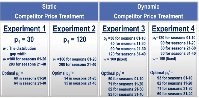
The theoretical model is the same as in Experiment 2. According to the parameters set, in the application of increasing competitive price (i.e. Experiment 3), the optimal price that the subjects should determine is 60 in seasons 01-10, 71 in seasons 11-20, 82 in seasons 21-30, 93 in seasons 31-40. Whereas in the application of decreasing competitive price (i.e. Experiment 4), the optimal price that the subjects should determine is 93 in seasons 01-10, 82 in seasons 11-20, 71 in seasons 21-30, and 60 in seasons 31-40.
(3.9)
(3.10)
(3.11) (3.12) (3.8)
12
4. EXPERIMENTAL SETUP
4.1. Theoretical Benchmarks of Experiments
The experiment scenarios are based on a one-class airline context (while observing the second airline’s competitive price decisions), because revenue management is frequently practiced in airline industry. The subjects acquire the role of an Airline Sales Director and they are asked to determine the price of economy class seats in order to maximize their revenue by observing the price of a competitor airline in the environment. The experiments are designed in such a way that environmental factors are gradually changing. The external parameters are initially kept simple and relatively static, and these parameters are gradually changed more and more to increase the complexity of decision-making environment. The experimental setup is summarized in Table 1. The static competitor price treatment is designed to limit the environmental parameters to one single variable, the distribution gap width, w. In the dynamic competitor price treatment, the distribution gap width is kept constant; however, this time, the competitor changes its price linearly by thirty monetary units in every ten seasons, respectively (Table 1).
13
In the first two experiments, the competitive price is static, with a low price level (y1=p1,11=30) and a high price level (y2=p1,2=120), respectively. The theoretical
benchmarks for Experiments 1 and 2 are summarized in Table 2.
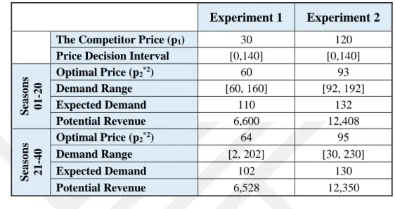
Table 2 Theoretical benchmarks for Experiments 1 and 2
Experiment 1 Experiment 2
The Competitor Price (p1) 30 120
Price Decision Interval [0,140] [0,140]
Seasons 01 -20 Optimal Price (p2*2) 60 93 Demand Range [60, 160] [92, 192] Expected Demand 110 132 Potential Revenue 6,600 12,408 Seasons 21 -40 Optimal Price (p2*2) 64 95 Demand Range [2, 202] [30, 230] Expected Demand 102 130 Potential Revenue 6,528 12,350
In the last two experiments, the competitive price is dynamic and subject to increase (y3=p1,3=30 → 120) or decrease (y4=p1,4=120 → 30) by thirty monetary units in every ten
seasons, respectively. The theoretical benchmarks for Experiments 3 and 4 are summarized in Table 3.
Table 3 Theoretical benchmarks for Experiments 3 and 4
Experiment 3 Experiment 4
Price Decision Interval [0,140] [0,140]
Seasons 01
-10
The Competitor Price (p1) 30 120
Optimal Price (p2*) 60 93 Demand Range [60, 160] [84, 184] Expected Demand 110 134 Potential Revenue 6,600 12,462 Seasons 11 -20
The Competitor Price (p1) 60 90
Optimal Price (p2*) 71 82 Demand Range [68, 168] [76, 176] Expected Demand 118 126 Potential Revenue 8,378 10,332 1 p
1,j=The price value “p1” determined by the competitive firm during seasons of Experiment “j”, j={1,2,3,4}
14 Seasons 21
-30
The Competitor Price (p1) 90 60
Optimal Price (p2*) 82 71 Demand Range [76, 176] [68, 168] Expected Demand 126 118 Potential Revenue 10,332 8,378 Seasons 31 -40
The Competitor Price (p1) 120 30
Optimal Price (p2*) 93 60
Demand Range [84, 184] [60, 160]
Expected Demand 134 110
Potential Revenue 12,462 6,600
In all four experiments the number of seats to be sold is fixed as 150 seats. The customer demand is randomly determined with respect to a discrete uniform distribution on the intervals given in the previous section. This form of demand function is broadly used in environments where two prices define the demand of some good (Akbay and Ayvaz Çavdaroğlu, 2000).
The “demand that subjects observe” and the “amount of seats sold” change according to the price (p2,j3) set by the airline sales director (i.e. the subject). If the realized demand
happens to be greater than the number of seats available, only as many as the total number of seats are sold.
4.2. Profile of Experiment Subjects
All experimental applications were carried out with a group of students from Kadir Has University and Istanbul Technical University. The subjects were chosen among a group of undergraduate students studying in business, international trade and finance, management information systems, industrial engineering, and civil engineering. Candidates were required to have taken and passed basic mathematics and statistics courses as a pre-condition to participate in the experiment. No statistical difference was observed between the experimental performances of students studying in different departments and/or different universities.
3 p
2,j=The average price value “p2” determined by the subject during seasons of Experiment “j”, j={1,2,3,4}
15 4.3. Recruitment Process of Experiment Subjects
Initial announcements to call for voluntary participants were delivered to students through posters posted on university boards and via Twitter social media account called “@hadigeloyna”. The poster design can be seen in Figure 1.
The students who were eligible to participate in the experiment were first sent instructions explaining the experiment via electronic mail. They were then asked to fill out a questionnaire to measure their risk appetite, their optimal search motives and their cognitive skills. After filling out the questionnaire, subjects were then invited to the experiment.
4.4. Organization of Experimental Sessions
The experimental sessions were held in the computer laboratories of Kadir Has University. Upon their arrival, subjects were first asked to sign a “Participant Consent Form” and their approval was obtained. Then, the experiment was thoroughly explained once again. The instructions given to the subjects during the experiments are included in Appendix B. It should be noted that the instructions are prepared in Turkish, since the experiments are carried out with subjects whose native language is Turkish.
Experimental sessions lasted an average of one hour; they were carried out by allowing each participant to play the game at the same time and without being affected by or speaking to each other.
16
17 4.5. Monetary Budget used for Experiments
Since the budget allocated to the subjects within the scope of the budget of the TÜBİTAK research project envisages to give an average of 50 Turkish Liras (TL), pilot experiments were made without the participation fee to a group of undergraduate students tutored by the thesis advisor. Pilot experiments showed that the total budget would be sufficient for conducting all experiments. In order to reach more participants for data collection, the net value of the participation fees is decided as 50 TL on average; the fee varying between 40, 50, 60 or 70 TL according to the subjects’ performance on total sales revenue. 4.6. Usage of Software for Data Collection
The experiments are conducted by using Visual Basic for Application (VBA) with Microsoft Office Excel software. The designed interface includes textboxes for the subject to input their name, their school number, and their price value for the corresponding season. The interface also informs the subject about the competitor’s price (p1), the number of available seats (150), the price (p2) range allowed to enter, as well as
the range of customer demand relative to the considered ticket price (p2).
In the middle of the screen there is a “Decision Support Tool”, which helps the subjects to conduct a “what-if” analysis by comparing the demand range to be determined by the ticket price and the corresponding revenue that can be potentially made as a result of possible demand values. The decision support tool provides a list of potential demand values increasing ten by ten, ranging between 0 and 150, i.e. the minimum and maximum number of seats available to be sold. The subject is able to see how many seats they would sell in case of which demand value, and how many seats would then be left empty. The revenue related to the potential demand values are also presented to the decision makers. Once the subject makes their decision, they finalize the price for the corresponding season by pressing the button entitled “Record Ticket Price”. An exemplary user interface can be observed in Figure 2. It should be noted that the interface is designed in Turkish language.
18
Figure 2 Sample user interface that subjects interact with during experiments 4.7. Statistical Methods Used for Data Analysis
There are three statistical methods used for analyzing the collected data. These are summarized in the following sub-sections:
4.7.1. The Two-Tailed Wilcoxon Signed Rank Test
The Wilcoxon Signed Rank Test is used in order to compare two sets of scores that come from the same sample. Our study contains a static competitor price treatment with two experiments, in which, the distribution gap width is widened at the second half of the treatment. Therefore, the data at the second half of this treatment is generated by the same sample, only with a change in environmental factor, (i.e. “w”). The Wilcoxon Signed Rank Test permits the researchers to investigate any change in revenues from the first half to the second half of the treatment, when subjects are faced with a changing environmental condition. The Wilcoxon Signed Rank Test reveals whether there was a difference in realized price average and/or realized revenue under two different demand variance.
For the Wilcoxon Signed Rank Test, both samples must be of equal size. This test is used for the generation of the majority of data presented in the upcoming tables, unless otherwise specified.
19 4.7.2. The Wilcoxon Rank-Sum Test
When the effects of personality traits are examined, the sample sizes of all four experiments are grouped into two distinctive sub-groups with respect to the subjects’ score on cognitive reflection skills, maximizing tendencies, and risk appetites. Because the two sub-groups rarely end up with equal sample sizes, The Wilcoxon Signed Rank Test can no longer be used for conducting a comparative analysis. Therefore, a test that allows comparing two samples with unequal sample sizes is needed, that is the very reason that the Wilcoxon Rank-Sum Test is employed in this study.
The Wilcoxon Rank-Sum Test (a.k.a. The Mann-Whitney U Test) compares whether there is a difference in the dependent variable for two independent groups. For these analyses, the dependent variable is the CRT, MT, and risk scores of the sub-groups. The test controls the distribution of the dependent variable and checks if it is identical in both sub-groups; the presence of identical distribution means that both samples come from the same population.
4.7.3. Linear Regression
Linear regression is an approach to model a relationship between a dependent variable and one or more independent variables. It is a widely-used regression analysis technique to fit a predictive model. This model can then be used when more values of independent variables are collected, in order to forecast the value of the dependent variable. In our study, the independent variables are CRT, MT and risk scores, and a predictive model is fitted in order to estimate future realized price or realized revenue values (i.e. dependent variables) with respect to personality traits, and the expected performance in making good predictions are shown with higher adjusted R-square values.
4.8. Sample Sizes of Experiments
Thirty-two subjects within the scope of Experiment 1 (low competitor price, 30) and thirty-three subjects within the scope of Experiment 2 (high competitor price, 120) participated in the experimental sessions held in the computer laboratories of Kadir Has University. As a result of these first analyzes, all of the experimental data were evaluated as usable, except one subject in Experiment 2. In other words, it was possible to collect healthy and reliable data from 32 and 32 subjects for Experiments 1 and 2 (Table 4).
20
Thirty-eight subjects within the scope of Experiment 3 (increasing competitor price, 30→120) and thirty-nine subjects within the scope of Experiment 4 (decreasing competitor price, 120→30) participated in the experimental sessions held in the computer laboratories of Kadir Has University. As a result of initial analyzes, one subject in Experiment 3 and two subjects in Experiment 4 were eliminated due to producing unreliable and/or contradictory data. All the remaining experimental data were evaluated as usable. In other words, it was possible to collect healthy and reliable data from 37 and 37 subjects for Experiments 3 and 4 (Table 4).
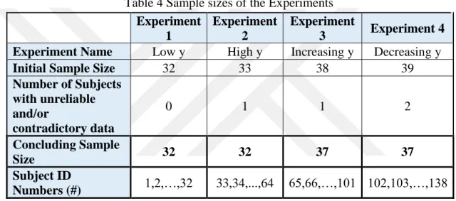
Table 4 Sample sizes of the Experiments
Experiment 1 Experiment 2 Experiment 3 Experiment 4
Experiment Name Low y High y Increasing y Decreasing y
Initial Sample Size 32 33 38 39
Number of Subjects with unreliable and/or contradictory data 0 1 1 2 Concluding Sample Size 32 32 37 37 Subject ID Numbers (#) 1,2,…,32 33,34,...,64 65,66,…,101 102,103,…,138 Each subject participated in exactly one experiment. The results obtained as a consequence of the analysis of these data can be summarized with the figures and tables in the following section.
21
5. EXPERIMENT RESULTS
5.1. Comparison of Experiment Results with Theoretical Benchmarks
This section presents the comparison of the experiments’ results with the theoretical benchmarks. Each subject’s experiment performance is averaged over forty seasons; therefore, each data point corresponds to the average performance of a single subject. The sample size “n” for the following hypothesis tests are the number of subjects in Experiments 1, 2, 3, and 4. (n1=n2=32, n3=n4=37). Comparisons are made thanks to the
usage of the two-tailed Wilcoxon signed rank test.
5.1.1. “Static Competitor Price” Treatment
Hypothesis 1: In the “static competitor price” treatment for both competitor price levels (y1=p1,14=30 or y2=p1,2=120), subjects’ pricing decisions (p2,j5) will be as predicted by
theory.
Table 5 is comparing the results of experiment performance with the theoretical benchmarks for the “static competitor price” treatment. In both Experiments 1 and 2, the realized price average is decreasing although the optimal price values are increasing. In the first twenty seasons of Experiment 1, the mean price value is rather close to the optimum value. However, the visualization in Figure 3 shows that the mean price during the second half of the experiment is decreasing although the optimal price is supposed to be larger. Therefore, human decision makers tend to fall further away from the optimal price values.
During first half of Experiment 2, subjects tend to determine even lower prices when compared with the optimum value. And as the visualization in Figure 4 reveals, at the second half, the mean price is still decreasing, although the median catches the optimum value (Table 5).
According to the results in Table 5, the subjects did not reach statistically different results from the optimal price on average. However, the actual revenue values deviated
4 p
1,j=The price value “p1” determined by the competitive firm during seasons of Experiment “j”, j={1,2,3,4}
5 p
2,j=The average price value “p2” determined by the subject during seasons of Experiment “j”, j={1,2,3,4}
22
significantly from the optimal values. The reason for this situation is that the subjects deviate a lot from the optimal in the positive and negative direction in their season-based decisions, while attaining the correct price on average. This situation is also observed in Figures 3 and 4. In the first experiment, the subjects set prices below and above 60 which is the optimal price in the first 20 seasons; in the second 20 seasons, they made price decisions generally below the correct price of 64. In the second experiment, the subjects made pricing decisions that are generally lower than 94 and 95, which are the optimal prices. The same situation is confirmed by individual analyzes shown in Table 6. In fact, although the subjects gave correct prices on average, they were only able to give the correct price individually by approximately 50%, sometimes 34-37%.
One can conclude that there is no sign of a significant learning effect in pricing decisions of subjects when the demand range widens. Except during the second half of Experiment 1, individual deviations are significant in both experiments due to high p-values in realized price averages (Table 5).
Table 5 Comparison results of experiment performance with the optimal thresholds in Experiments 1 and 2
An individual level analysis presented in Table 6 reveals that pricing decisions of subjects tend to vary even more, when the demand range is largened. This is another sign of the lack of learning effect, that one would expect to see. The average price over the periods for experiment 1, visualized in Figure 3, show that there are significant deviations even on the seasonal average level. At the first half of the experiment, the average price fluctuates above and below the optimum price, and at the second half, the average price
N Min Max Mean Std. Dev. Median
Seasons 01-20 32 41.45 84.65 60.6031 9.5168 60.25 60.00 0.6671270
Seasons 21-40 32 33.75 89.70 59.1813 12.4556 60.10 64.00 0.0225290
Seasons 01-20 32 73.40 117.90 92.4906 11.1540 92.25 94.00 0.2950000
Seasons 21-40 32 49.00 116.85 91.4797 14.6640 94.93 95.00 0.2780950
N Min Max Mean Std. Dev. Median
Seasons 01-20 32 4,177.89 6,190.40 5,749.12 463.14 5,919.30 6,600.00 0.0000008
Seasons 21-40 32 4,065.00 6,965.29 5,825.90 621.82 5,953.76 6,528.00 0.0000040
Seasons 01-20 32 9,094.05 11,466.20 10,642.99 652.28 10,875.38 12,408.00 0.0000008
Seasons 21-40 32 7,004.25 11,620.00 10,115.16 814.77 10,340.73 12,350.00 0.0000008
Experiment Data Optimal
Price P-value Realized Price Average Experiment 1 (Low y=30) Experiment 2 (High y=120)
P-values are obtained from two-tailed Wilcoxon signed ranked test. [Sample size is 32 for low y=30 and for high y=120.]
Experiment Data Potential
Revenue P-value Realized Revenue Experiment 1 (Low y=30) Experiment 2 (High y=120)
23
consistently falls under the optimum. A similar observation applies to Experiment 2, as displayed in Figure 4.
Table 6 Individual level comparison of pricing decisions with the optimal in Experiments 1 and 2
Figure 3 Average price over the periods for Experiment 1
Figure 4 Average price over the periods for Experiment 2
P Value ≤ 0.05 P Value > 0.05 Total
Seasons 01-20 17 15 32 Seasons 21-40 11 21 32 Seasons 01-20 12 20 32 Seasons 21-40 16 16 32 Experiment 1 (Low y=30) Realized Price Average Experiment 2 (High y=120) Realized Price Average # of Subjects with
24
Overall, Hypothesis 1 found rather weak support on the average data; besides, the individual level analysis indicated that the hypothesis is again weakly supported. It is because, not only in the first experiment (y = 30), the average price is lower than optimal, but also in the second experiment (y = 120) the average price is still lower. On top of that, human decisions cause the average price to decrease further in the second half of both experiments.
Hypothesis 2: In the “static competitor price” treatment for both competitor price levels, subjects’ realized revenues will be as predicted by theory.
In terms of realized revenue, the mean realized revenue values fall behind the potential revenue values in both experiments. Although one can see the positive signs of a learning effect in terms of an increased realized revenue, when comparing the mean values at the first and second half of Experiment 1, the difference between theoretical prediction and the realized revenue average are significant.
When there is no significant deviation from the optimal prices and the demand is random instead of being consistently lower than expected, the presence of low realized revenues indicates that pricing is consistently incorrect. Even though subjects gave the correct price on average, the total revenue remained low due to season-to-season variations. Since realized demand values are determined under a discrete uniform distribution, the visualization of demand values in Figure 5 and Figure 6 is logical and predictable. Thanks to the discrete uniform distribution of demand values, one can observe the presence of realized revenues approximate to the potential revenues, as depicted in Figure 7. The mean realized revenue at the second half of experiment 2 is even less than the mean at the first half, this trend can also be observed in Figure 8.
The terms used in Figures 7 and 8 are defined as follows. “Realized Revenue” is calculated by multiplying the realized price average and the realized demand average in corresponding season. “Potential Revenue” is calculated by multiplying the theoretically optimal price and the theoretically expected demand for the corresponding season. Lastly, “Optimal Realized Revenue” is the value obtained by multiplying the theoretically optimal price and the realized demand average in corresponding season.
25
Figure 5 Average demand over the periods for Experiment 1
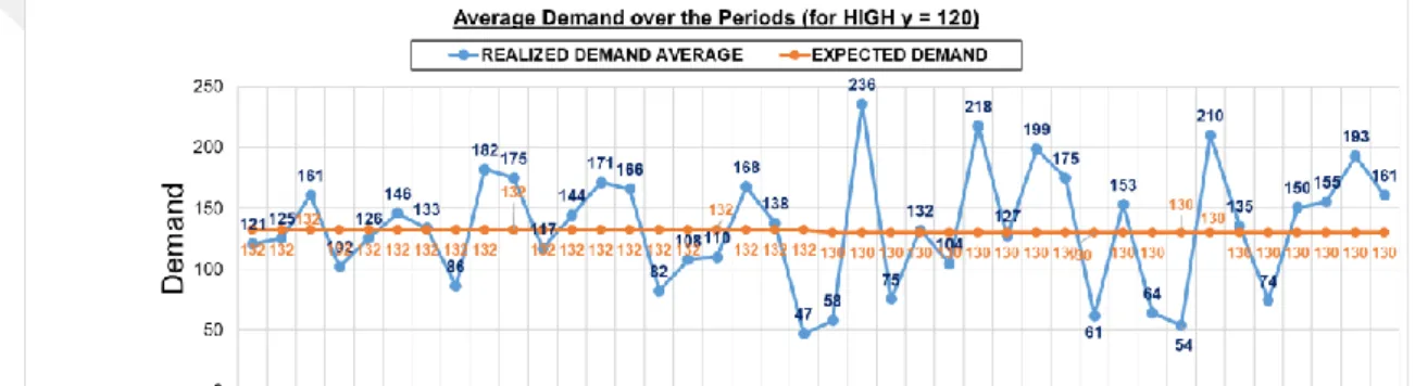
Figure 6 Average demand over the periods for Experiment 2
26
Figure 8 Average revenue over the periods for Experiment 2
Consequently, since realized revenue averages consistently fail to reach the potential revenue values, Hypothesis 2 is strongly rejected.
Hypothesis 3: The value of the competitive firm price given in the “static competitor price” treatment for both competitor price levels (y1=p1,16=30 or y2=p1,2=120), do not
affect the pricing decisions (p2,j7) determined by the subjects.
Since no significant anchoring effect was observed in the “static competitor price” treatment for both competitor price levels, Hypothesis 3 is accepted.
Hypothesis 4: The increase in the variance of the demand distribution in the second twenty seasons of the “static competitor price” treatment, do not affect the pricing decisions of the subjects.
Hypothesis 4 is rejected; because in both Experiments 1 and 2, the subjects set prices such that the deviation from optimal value is more significant in the second 20 seasons
6 p
1,j=The price value “p1” determined by the competitive firm during seasons of Experiment “j”, j={1,2,3,4}
7 p
2,j=The average price value “p2” determined by the subject during seasons of Experiment “j”, j={1,2,3,4}
27
(Figures 3, 4). In addition, the p-values and average prices of pricing decisions in Table 5 are lower for the second 20 seasons. In addition, Table 6 shows that the proportion of correct prices in the first 20 seasons decreased considerably (but in the second trial, the opposite is weakly observed). These findings lead the researchers to reject Hypothesis 4 and to conclude that as the variance increases, pricing decisions made will deviate more from the optimal.
5.1.2. “Dynamic Competitor Price” Treatment
Hypothesis 5: In the “dynamic competitor price” treatments, for both increasing and decreasing price trends (y3=p1,3=30→120 or y4=p1,4=120→30), subjects’ pricing
decisions (p2,j) will be as predicted by theory and they will not be biased by the trend of
the competitor price.
When the realized price averages of Experiment 3 (increasing y3=p1,3=30→120) in Table
7 are analyzed, the first detection is the fact that anchoring effect is observed over the price of “y”. Although the mean price values between seasons 01-10 and 11-20 fall under the optimum values of 60 and 71, respectively; when the optimum “y” is equal to 82 between seasons 21-30, subjects tend to increase their price average up to 5 units above the optimum. Between seasons 31-40, subjects behave more and more aggressively to the changes in “y” by increasing the average up to ten units above the optimum. This trend is obviously observed in Figure 9.
Similarly, results of Experiment 4 (decreasing y4=p1,4=120→30) confirms this aggressive
tendency. Between seasons 01-10, the price determined by subjects is on average 5 units above the optimum. Seasons 11-20 realize an average almost equal to the optimum price, showing a consistency with the theoretical optimal. As the competitor firm decreases their price (“y”) even further, the mean value of the subjects show a dramatic decrease, 11 units lower than optimum between seasons 21-30 and 20 units lower than the optimum in seasons 31-40, proving the presence of the anchoring effect over the price of “y”. In other words, as the competitor firm updates its price in a linear trend, the human subjects become more likely to make less rational pricing decisions in order to attract more customers (or to minimize the impact of losing customers). This trend is also obvious in
28
Figure 10. The last quarters of Experiment 4 has a minimum realized price average of 13.40 (subject id#129) that proves the willingness of human subjects to increase demand for their product by decreasing their price over the competitive firm.
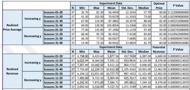
Table 7 Comparison results of experiment performance with the optimal thresholds in Experiments 3 and 4
When Table 8 demonstrating the “individual level comparison of pricing decisions with the optimal” is analyzed, it is observed that the p-value in second, third and fourth quarters of Experiment 3 is increasing, meaning that the number of decision makers who set prices closer to optimum in Experiment 3 is increasing. However, the p-values in realized price average section of Table 7 demonstrates that on average prices are deviating more from the optimal in these quarters. This means that the decision makers who made wrong pricing decisions deviated significantly from the optimal value, which affected the average prices of the entire subject group.
N Min Max Mean Std. Dev. Median
Seasons 01-20 37 35.70 81.30 56.4459 12.1014 57.70 60.00 0.122006000000 Seasons 11-20 37 41.30 105.00 70.8378 11.1933 73.00 71.00 0.825909000000 Seasons 21-30 37 67.00 116.90 87.3865 10.3579 88.60 82.00 0.005252000000 Seasons 31-40 37 69.00 128.90 103.8054 13.2368 103.50 93.00 0.000096000000 Seasons 01-20 37 77.00 135.80 97.1946 11.1159 97.40 93.00 0.026745000000 Seasons 11-20 37 66.40 95.70 82.4541 7.4158 83.60 82.00 0.618562000000 Seasons 21-30 37 46.30 77.50 60.6027 7.6690 61.10 71.00 0.000000457690 Seasons 31-40 37 13.40 72.50 40.8162 13.0824 41.70 60.00 0.000000416080
N Min Max Mean Std. Dev. Median
Seasons 01-20 37 4,798.80 6,423.60 5,877.56 457.7438 6,087.00 6,600.00 0.000000114020 Seasons 11-20 37 6,022.44 8,364.50 7,935.12 553.9635 8,124.90 8,378.00 0.000000114020 Seasons 21-30 37 7,367.89 10,042.50 9,612.23 460.5722 9,696.60 10,332.00 0.000000114020 Seasons 31-40 37 7,733.60 12,134.10 10,815.38 1,105.4162 10,955.00 12,462.00 0.000000114020 Seasons 01-20 37 6,104.22 11,651.00 10,777.75 997.1652 11,101.90 12,462.00 0.000000114020 Seasons 11-20 37 7,885.00 9,725.50 9,304.94 425.7017 9,402.70 10,332.00 0.000000114020 Seasons 21-30 37 6,242.50 7,875.00 7,344.71 385.8811 7,294.10 8,378.00 0.000000113970 Seasons 31-40 37 2,010.00 6,516.90 5,117.73 1,072.3149 5,589.80 6,600.00 0.000000114020
P-values are obtained from two tailed Wilcoxon signed ranked test. [Sample size is 37 for both "increasing y" and "Decreasing y".]
Experiment Data Potential
Revenue P Value
Realized Revenue
increasing y
Decreasing y
Table 3: Comparison results of experiment performance with the optimal thresholds (SD)
Realized Price Average
increasing y
Decreasing y
Experiment Data Optimal
29
Table 8 Individual level comparison of pricing decisions with the optimal in Experiments 3 and 4
Data in Table 8 show that in Experiment 4 (“decreasing y”), 35 subjects out of 37 made the wrong decision in the third quarter, by persistently setting a very low price. This persistence can be proved by the low standard deviation in Table 7, the line corresponding to “decreasing y, seasons 21-30” (7.6690). This observation is another proof that demonstrates the wrongful judgements of human decision makers are widely present and; not only subjects are wrong, but they are also persistent in making those wrong decisions over and over again.
Figure 9 Average price over the periods for Experiment 3
P Value <= 0.05 P Value > 0.05 Total
Seasons 01-20 21 16 37 Seasons 11-20 15 21 37 Seasons 21-30 10 27 37 Seasons 31-40 8 29 37 Seasons 01-20 14 23 37 Seasons 11-20 17 20 37 Seasons 21-30 35 2 37 Seasons 31-40 34 3 37
increasing y Realized Price Average
Decreasing y Realized Price Average
Table 4: Individual level comparison of pricing decisions with the optimal (SD) # of Subjects with
30
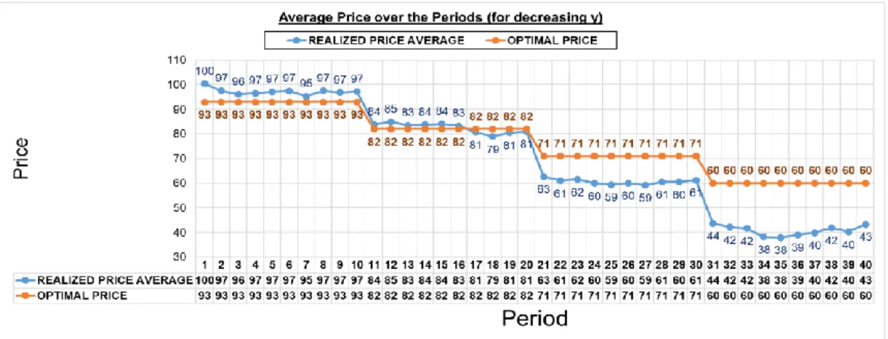
Figure 10 Average price over the periods for Experiment 4
Consequently, the following judgment can be reached: If the price is not changing dynamically, no matter if the competing firm’s price is low or high, human subjects successfully get closer to the optimal price. In a dynamic price setting, if the rival’s price is constantly changing, the aggressiveness of human subjects is increasing and human decisions are going away from optimal values more and more.
Therefore, Hypothesis 5 is to be rejected. In the “dynamic competitor price” treatments, for both increasing and decreasing price trends (y3=p1,3=30→120 or y4=p1,4=120→30),
subjects’ pricing decisions (p2,j) are not as predicted by theory (human decisions are
biased by the trend of a dynamic competitor price).
Hypothesis 6: In the “dynamic competitor price” treatment for both competitor price trends, subjects’ realized revenues will be as predicted by theory.
Since realized demand values are determined under a discrete uniform distribution, the realized values randomly fall above or below the expected values. Hence, the visualization of demand values in Figure 11 and Figure 12 is logical and predictable. Thanks to the discrete uniform distribution of demand values, one can observe the presence of realized revenues fluctuating above or below the potential revenues, as depicted in Figure 13 and Figure 14. Although there is constant fluctuation, the mean realized revenues almost always fall short of potential revenues, both in experiment 3 and in experiment 4. The realized revenue section of Table 7 show this short-falling when the columns of “Mean” and “Potential Revenue” are compared against each other. In spite of
31
all, Figure 13 depicts an increasing trend in realized revenues from season 1 up until season 40. Likewise, a decreasing trend in realized revenues can also be observed in Figure 14.
In terms of realized revenue values depicted in Table 7, both in experiments 3 and 4 (“increasing y” and “decreasing y”), the third quarter to the fourth quarter, standard deviations triple, meaning the tendency to aggressiveness in making wrong decision increases. Low p-values in Table 7 also prove that realized revenues are significantly different from theoretical optimum values.
Figure 11 Average demand over the periods for Experiment 3
32
Figure 13 Average revenue over the periods for Experiment 3
Figure 14 Average revenue over the periods for Experiment 4
As a result, Hypothesis 6 is strongly rejected, because in the “dynamic competitor price” treatment for both competitor price trends, subjects’ realized revenues are not realized as predicted by theory.
Hypothesis 7: The value of the competitor firm’s price given in the “dynamic competitor price” treatment (y3=p1,3=30→120 or y4=p1,4=120→30), do not affect the pricing
decisions (p2,j) determined by the subjects.
When the realized price averages of Experiment 3 (increasing y3=p1,3=30→120) in Table