Statistical evaluation of maximum displacement demands of SDOF systems by code-compatible nonlinear time history analysis

(1)

Contents lists available atScienceDirect

Soil Dynamics and Earthquake Engineering

journal homepage:www.elsevier.com/locate/soildyn

Statistical evaluation of maximum displacement demands of SDOF systems

by code-compatible nonlinear time history analysis

Ali Haydar Kayhan

a

_{, Ahmet Demir}

a

_{, Mehmet Palanci}

b,⁎ a_{Department of Civil Engineering, Pamukkale University, Denizli, Turkey}

b_{Department of Civil Engineering, Istanbul Arel University, Istanbul, Turkey}

A R T I C L E I N F O Keywords:

Displacement demands Ground motion record sets Nonlinear time history SDOF systems Statistical evaluation

A B S T R A C T

By the developments in structural and earthquake engineering, modern seismic codes have begun to recommend nonlinear static and dynamic procedures to approximate the maximum displacement demands which have ut-termost importance for seismic assessment of buildings. Dynamic procedure is the most accurate and reliable among them and requires the selection of real/artificial ground motion records compatible to considered elastic design spectra. In this study, maximum displacement demands of SDOF systems with various lateral strength ratios and vibration periods are determined via nonlinear time history analyses using the code-compatible different records sets constructed by real accelerograms. For this purpose, 30 ground motion record sets com-patible with elastic design spectra defined for each local soil class in Turkish Earthquake Code are used sepa-rately. Evaluations have highlighted that i) variation of maximum displacement demands in the sets are high; ii) Distinct ground motion record sets may result in different displacement demands even though they are com-patible with the same design spectra; iii) maximum displacement demands of different ground motion record sets can be simply accepted as random samples of the same population at 95% confidence level. In addition to dynamic analysis results, maximum displacement demands of static procedure are determined for the same target spectra and results of both methods are compared. Comparisons showed that special attention should be made to static procedure estimations for the buildings with long periods on stiff soils. Finally, linear regression models, depending on the fundamental periods for each lateral strength ratio and soil type, are proposed for rapid prediction of displacement demands in reliability based manner.

1. Introduction

Performance-based design is currently the popular design philo-sophy in which design criteria are expressed in terms of achieving stated performance objectives when the structure is subjected to re-quired levels of seismic hazard[1]. Performance objectives can be de-pended on the level of damage to the structure, which in turn can be related to displacement and drift. Thus, structural response parameters such as maximum displacement, global or interstory drift ratio, ducti-lity demands, etc. have been widely used as design targets [2,3]. In order to identify various performance levels for the seismic perfor-mance evaluation of existing buildings, similar parameters are also utilized[4,5].

In order to estimate the response of structures to seismic excitation, nonlinear time history analysis of three-dimensional structural models is the most comprehensive and accurate method. However, it can be said that nonlinear time history analysis of three-dimensional structural

models are complex and difficult. For this reason, many research efforts have focused on simpler approaches. Using equivalent single degree of freedom (SDOF) system is one of the simpler approaches. SDOF systems have been preferred as structural models to estimate and evaluate the response of structures to seismic excitation[6–13]. In these studies, various criteria are used in the selection of ground motion records for nonlinear time history analyses.

Nowadays, thanks to easily accessible digital ground motion data-base, real ground motion records are increasingly preferred for time history analysis. It should be noted that ground motion records vary based on magnitude of the earthquake, faulting type, local soil prop-erties, the distance between the site and recording station, etc. In ad-dition, ground motion records used for time history analysis directly affect the response parameters such as displacements or drift demands that would be considered for seismic design or evaluation of structures. Thus, selection of ground motion records based on the seismicity of the region and the local soil conditions that a structure located is important

https://doi.org/10.1016/j.soildyn.2018.09.008

Received 23 September 2017; Received in revised form 1 May 2018; Accepted 9 September 2018

⁎_{Corresponding author.}

E-mail addresses:hkayhan@pau.edu.tr(A.H. Kayhan),ademir@pau.edu.tr(A. Demir),mehmetpalanci@arel.edu.tr(M. Palanci).

Available online 02 October 2018

(2)

for accurate estimation of the seismic behavior of that structure in a possible earthquake[14–17].

Time history analysis is accepted as one of the structural analysis method for seismic design or performance evaluation by modern seismic design codes[18–21]. Turkish Earthquake Code (TEC)[22]is one of the design codes. In these codes, relatively similar procedures with minor differences for simulating the seismic actions are described. For example, seismic loads are represented by ground motion records used for time history analyses. Synthetic, artificial, or real ground motion records could be used as long as they are compatible with re-gional design spectra defined in the seismic codes within a stated period range. The mean of the structural responses can be used for seismic design and/or performance evaluation if at least seven ground motion records are selected, otherwise the maximum of structural responses is considered[23–25].

It is possible to obtain various code-compatible ground motion re-cord sets by selecting and scaling from hundreds of ground motion records in digital databases[16,26–28]. As mentioned earlier, ground motion records used for time history directly affect the displacement and/or drift ratio demands that would be considered for seismic design or performance evaluation. Hence, seismic demands could be accepted as random variables that vary according to ground motion record sets used for time history analyses. Moreover, modern seismic codes con-sider only the mean spectrum of selected ground motion records and target design spectrum for compatibility without considering random variability of the individual ground motion records. For this reason, the dispersion of seismic demands obtained using code-compatible ground motion record sets is generally high[29–31].

The aim of this study is to statistically evaluate the central tendency and dispersion of maximum displacement demands of SDOF systems using different code-compatible ground motion record sets. 21 different SDOF systems with various vibration periods and lateral strength ratio are used in order to consider a broad range of SDOF systems. Ground motion record sets compatible with design spectra described for local soil classes defined in TEC are used for nonlinear time history analyses. For each local soil class, 30 different ground motion record sets are used to obtain statistically significant number of random samples. Performing nonlinear analysis of the SDOF system, maximum dis-placement demands are calculated for each of the ground motion re-cords in the record sets. Then, the mean of maximum displacement demands are calculated for each of the record sets. Coefficient of var-iation is used to numerically evaluate the dispersion of the displace-ment demands within the records sets. One-way analysis of variance is also used to evaluate the difference between the mean of the dis-placement demands of the record sets compatible with the same design spectra. The problem of estimating the displacement demands for seismic design and performance evaluation has attracted growing at-tention in recent years. In this study, confidence intervals of displace-ment demands for each of the SDOF systems and local soil classes are estimated at 95% confidence level. Linear regression models, depending on the fundamental periods for each lateral strength ratio and soil type, are also proposed for rapid prediction of displacement demands in re-liability based manner.

2. Elastoplastic SDOF systems

Actually, all the structures possess infinite number of degrees of freedom and are called as multi degree of freedom (MDOF) systems. Nowadays, nonlinear response of MDOF systems to seismic excitation can be estimated through three-dimensional nonlinear time history analysis. However, time history analysis of the structures with a large number of degrees of freedom may require a significant amount of time. For this reason, a number of research efforts have focused on simple procedures to estimate the structural response of MDOF systems under seismic actions. For example, an equivalent SDOF system can be used as a basis for estimating the response of a MDOF model of the structures

[4]. In this way, the nonlinear response of the structures can be esti-mated from the response of equivalent SDOF system.

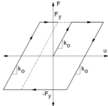
The mechanical model of a SDOF system subjected to seismic ex-citation is given inFig. 1. Equation of motion of a SDOF system is given in Eq.(1). In Eq.(1), k is the lateral stiffness of the system, c is the viscous damping coefficient and m is the mass of the system.

+ + =

mu cu ku mug (1)

When subjected to severe excitations such as strong earthquake ground motion, structures would respond inelastically and exhibit hysteretic behavior. Eq.(1)can be readily extended to inelastic systems. For such systems, the equation of motion is given in Eq.(2). In Eq.(2), F (u) is the resisting force of inelastic system.

+ + =

mu cu F u( ) mug (2)

Hysteretic models have been used for the inelastic earthquake-re-sistant design of structures[32]. The most commonly used model for describing the nonlinear hysteretic restoring force-displacement beha-vior is the perfectly elastoplastic model with no stiffness and strength degradation. This model is parameterized by yield force (Fy) and initial stiffness (k0). InFig. 2, force-displacement relationship for elastoplastic model is given. In this study, the SDOF systems are characterized by perfectly elastoplastic cyclic behavior. It should be noted that different hysteretic models can be used to represent the behavior of different type of structures subjected to earthquake motions.

A robust method for the estimation of the fundamental period of vibration is essential both for the design of new buildings and the performance assessment of existing ones. Several design codes provide formulas for estimating the fundamental period of buildings. Typically, such formulas are derived from regression analysis of numerical values, which have been obtained from measured periods of vibrations of real buildings during past earthquakes. Despite the fact that several other parameters affect the period of vibration, the formulas given by design codes are, typically, a function of the building’s height or the number of stories. For example, according to EUROCODE-8 [19], fundamental period of vibration and height (in meters) of the buildings relationship given in Eq.(3)is specified for force-based design of the moment re-sistant concrete frames with heights of up to 40 m. Similar relationship (see Eq.(4)) is specified in ASCE 07-05[20]. In NEHRP-94[33]and National Building Code of Canada (NBCC)[34]an alternative formula given in Eq.(5)is recommended for RC buildings based on the number

Fig. 1. Mechanical model of a SDOF system subjected to seismic excitation.

(3)

of stories, N: = T 0.075H0.75 ₍₃₎ = T 0.0466H0.9 (4) = T 0.1N (5)

If the Eqs.(3)–(5)are carefully examined, it can be deduced that RC buildings with 10 stories and/or 30 m in height or less have the funda-mental period equal or less than 1.0 s. These buildings also constitute an important part of existing RC buildings. In addition to fundamental period of the buildings, lateral strength ratio of the building, the ratio of the yield force to seismic weight of the building (Fy/W), should be de-termined to perform nonlinear time history analysis. Evaluation of var-ious studies in lateral strength ratio of low and mid-rise buildings have indicated that this ratio generally range between 0.1 and 0.3[35–37].

In order to obtain structural analysis results which can represent the structural response of low and mid-rise RC buildings up to 10 stories, natural vibration period of the SDOF systems used in this study is se-lected between 0.4 s and 1.0 s with increments of 0.1 s and the lateral strength ratio of the SDOF systems used in this study is selected as 0.1, 0.2 and 0.3.

3. Ground motion record sets

In most of the modern seismic codes including the Turkish Earthquake Code[22]time history analysis is accepted as one of the analysis method for design and/or performance evaluation, and re-quired conditions are defined (FEMA-368 [18], EUROCODE-8 [19], ASCE 07-05[20], GB[21]). In these codes, in order to simulate the seismic actions to be used as dynamic loading, relatively similar pro-cedures are described. According to these codes, the mean response spectra of the selected ground motion records for time history analysis should be compatible with the regional design spectra defined in the codes within a stated period range[23].

In this study, ground motion records compatible with TEC used for time history analysis of the SDOF systems. Elastic design spectra de-fined in TEC for each local soil class is considered separately to select ground motion record sets. European Ground Motion Database[38]is used to select real ground motions for the record sets.

3.1. Time history analysis requirements in TEC

According to TEC, in order to perform linear or nonlinear time history analysis of buildings previously recorded, artificially generated or simulated ground motions can be used. Recorded and simulated ground motions should be obtained by considering appropriate local site conditions. Moreover, ground motion records should meet the following conditions:

•

The duration of strong motion part shall be equal or bigger than 5 times the fundamental vibration period of the building in the con-sidered direction and 15 s;

•

Mean spectral acceleration of ground motion records for zero period shall be equal or bigger than design ground acceleration;

•

Mean spectral accelerations of ground motion records for 5% damping ratio shall be equal or bigger than 90% of design spectral accelerations in the period range between 0.2T and 2.0T with re-spect to fundamental vibration period T of the building in the con-sidered direction.

In time history calculations, at least three ground motions shall be used. The mean structural responses can be considered for the design or seismic performance evaluation if at least seven ground motions are utilized. Otherwise, the maximum of structural responses shall be considered.

3.2. Ground motion database and record sets

Four seismic zones (1st, 2nd, 3rd and 4th degree seismic zones), depicted in Seismic Zoning Map of Turkey prepared by the Ministry of Public Works and Settlement[39]are cited in TEC. Effective ground acceleration is 0.4g, 0.3g, 0.2g and 0.1g for the 1st, 2nd, 3rd and 4th degree seismic zones, respectively for a probability of exceedance of 10% in 50 years (for a return period of 475 years). In TEC, four local soil classes (Z1, Z2, Z3, and Z4) are defined. InTable 1, the information about local soil classes defined in TEC and EUROCODE-8 is given. Depending on the considered seismic zone and local soil class the elastic design spectrum are described to determine seismic loads.

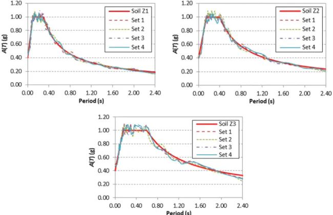
In this study, the 1st degree seismic zone is considered to account for high seismic regions. Spectral Acceleration Coefficient A(T) that would be used to calculate seismic loads based on the TEC specifications for the 1st seismic zone and local soil classes are demonstrated inFig. 3.

In order to obtain ground motion record sets, first, a catalog of ground motion records is obtained by selecting ground motion records from the European Strong Motion Database following these criteria: the epicentral distance of the record stations be in the range of 10–50 km; the magnitude of the source earthquake be greater than 5.5; and the peak ground acceleration of the ground motion records be 0.10g and higher. As known, five soil classes are defined in EUROCODE-8; A, B, C, D and E. In European Strong Motion Database, there is not sufficient number of ground motion records from soil class D and E satisfying the considered criteria. Thus, these soil classes are ignored in this study and

Table 1

Description soil classes according to EUROCODE-8 and TEC.

Definition Shear wave velocity (m/s) Soil class

EC-8 TEC EC-8 TEC EC-8 TEC

Rock or other rock-like geological formation Very dense sediment, gravel and solid clay > 800 > 700 A Z1 Very dense sand or gravel or very stiff clay Dense sediment gravel, very stiff clay 360–800 300–700 B Z2 Dense or medium dense sand, gravel or stiff clay Medium dense sediment and gravel, stiff clay 180–360 200–400 C Z3 Loose to medium cohesionless soil or soft to firm cohesive soil Weak sediment, soft clay alluvial layer with high water level < 180 < 200 D Z4

Surface alluvium layer C or D with water level on stiffer material E

(4)

only soil class A, B and C are considered to obtain the ground motion catalog. A total of 542 horizontal components of 271 ground motion records are selected for the catalog. Ground motion records in the catalog are grouped based on the soil class that they are recorded on. There are 190 horizontal components of 95 ground motion records, 236 horizontal components of 118 ground motion records, and 116 hor-izontal components of 58 ground motion records for soil class A, B and C, respectively, in the catalog. It can be seen from theTable 1that A, B, C soil classes correspond to Z1, Z2 and Z3 soils classes, respectively.

Ground motion record sets are obtained by selecting ground motion components from the catalog. The detailed information about ground motion selection procedure performed in this study can be found in Kayhan et al. [16]and Kayhan[28]. As mentioned before, recorded ground motions to be used for time history analysis should be obtained considering appropriate local site conditions according to TEC. For this reason, ground motion records sets compatible with soil classes Z1, Z2 and Z3 are obtained by selecting the ground motion records from the catalog considering relevant soil classes A, B and C, respectively.

The scaling coefficient for ground motion records is constrained to be in the range of 0.50–2.00. As the vibration period of the SDOF system is assumed to be range between 0.40s and 1.00s, compatibility of mean and target spectrum should be considered in the period range of 0.08–2.00s according to requirements given in TEC (Section 3.1). For each considered soil class, 30 ground motion record sets are obtained. Each set has seven ground motion components.

InFig. 4, mean spectra of ground motion records in the record sets and corresponding target spectra are given in order to show the com-patibility between mean and target spectra. It should be noted that four of the 30 record sets for each local soil class are selected as examples to show the compatibility.

The information about all the ground motion record sets is given in Appendix A.Appendix Aincludes ground motion record number, hor-izontal component indices and scaling coefficient. Detailed information about the ground motion records in the sets including record number, source earthquake, date of source earthquake and record station is also given inAppendix B.

4. Statistical evaluation of time history analysis results 4.1. The mean and dispersion of maximum displacement demands

Performing nonlinear time history analysis using ground motion records in the record sets, maximum displacement demands (Δmax) for the SDOF systems are calculated. InFig. 5, Δmaxvalues of 30 ground motion sets for soil Z1 and the SDOF system with T = 0.4 s and Fy/ W = 0.1 as a representative example. As can be shown from the figure, for each of the ground motion records in a record sets, various Δmax values are calculated. According to TEC, mean values of the seismic demands can be used if at least seven ground motion records used for time history analysis. Hence, mean of the seven Δmaxvalues (mΔ) are also calculated for each of the record sets. InFig. 5, mΔvalues of the record sets are also given as connected by a continuous line.

As shown from theFig. 5, different values of mΔare calculated for 30 ground motion record sets although the record sets are compatible with the same design spectrum. For example, value of mΔis 5.13, 5.63, 5.37 and 6.73 cm for Set 1, Set 2, Set 3 and Set 4, respectively. It can be said that there is also a significant dispersion of Δmaxvalues around the mΔvalues in each of the record sets.

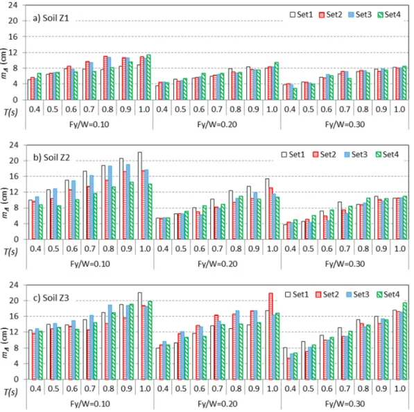
InFigs. 6a-6c, values of mΔof first four representative ground motion record sets are given for all the considered SDOF systems and local soil classes. mΔvalues calculated for all the SDOF systems and ground motion records sets can be found inAppendix C. According toFigs. 6a-6c, dif-ferent values of mΔ are calculated for a SDOF system using different ground motion record sets although the record sets are compatible with the same design spectrum. For example, for the SDOF system with T = 0.5 s and Fy/W= 0.1, mΔvalues of the first four record sets are 6.49, 6.68, 6.91 and 6.92cm for soil Z1, 12.60, 10.23, 12.86 and 8.40 for soil Z2, and 13.99, 12.79, 14.26 and 13.11cm for soil Z3. As expected, mΔ values increase when soil class changes from Z1 to Z3. This is valid for all the SDOF systems. In this study, well-known effects of T and Fy/W on displacement demands of structures are also observed. As can be shown clearly fromFigs. 6a-6c, values of mΔincrease with increasing T of the SDOF systems and decrease with increasing Fy/W of the SDOF systems.

(5)

In order to numerically evaluate the dispersion of Δmaxaround the mΔ, coefficient of variation (CoVΔ), ratio of standard deviation to mean, is calculated for each of the record sets. Values of CoVΔcalculated for all the record sets are given inAppendix C. InFig. 7, representative sam-ples for values of CoVΔare illustrated. The SDOF systems with minimum and maximum T and Fy/W are selected as representative samples. Considering the SDOF system with minimum T (0.4s), CoVΔvalues of 30

ground motion record sets randomly vary between 0.315 and 1.339, 0.463–1.677 and 0.545–1.255 for soil Z1, Z2 and Z3, respectively (Fig. 7a). InFig. 7b, CoVΔvalues for the SDOF system with maximum T (1.0s) are given. These values also vary between 0.368 and 0.876, 0.332–1.085 and 0.433–1.009 for soil Z1, Z2 and Z3, respectively.

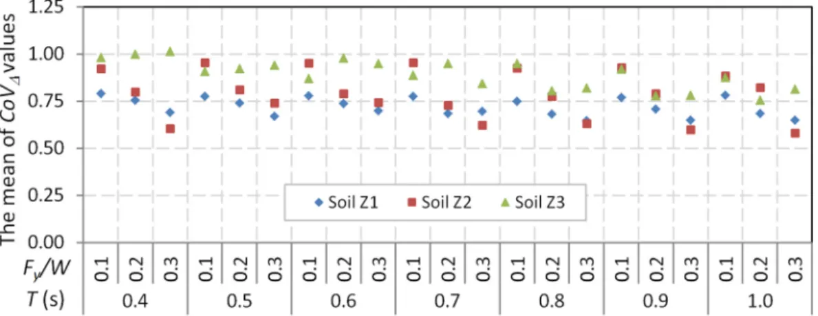
The central tendency of variation of the maximum displacement demands in the record sets is also evaluated. For this purpose, the mean

Fig. 5. Δmaxvalues calculated for SDOF system with T = 0.4 s, Fy/W = 0.1 (Soil Z1).

(6)

of the CoVΔvalues of 30 ground motion record sets are calculated for each of the SDOF systems and local soil classes, separately. As can be shown inFig. 8, these values change between about 0.50 and 1.00. This result numerically indicates that dispersion of the Δmaxaround the mΔis remarkably high and valid for all the SDOF system and local soil classes considered in this study. Similar result has also been stated that by Iervolino et al.[40], Catalan et al.[14], Sextos et al.[29], Katsanos and Sextos[30] and Ergun and Ates[41]for code-compatible nonlinear time history analysis. In this study, the remarkably high variation of the maximum displacement demands obtained from code-compatible non-linear time history analysis are observed for the broad range of SDOF systems with various T and Fy/W.

4.2. One-way analysis of variance

The results summarized inFig. 5andFig. 6show that different mΔ values can be obtained for a SDOF system using different ground motion record sets although the record sets are compatible with the same design spectrum. Therefore, it can be said that mΔis random variables depending on ground motion record sets used for nonlinear time history analysis.

There are several methods and/or parameters to be used to statis-tically evaluate the differences between mΔ values calculated for dif-ferent ground motion record sets. In this study, one-way analysis of variance (ANOVA) is used Gamst et al.[42]. The one-way ANOVA is used to evaluate whether there are any statistically significant differ-ences between the means of several independent groups. Suppose k independent groups drawn different populations, each of size n. The members of the groups are assumed as normally distributed with

Fig. 7. CoVΔvalues calculated for ground motion record sets.

(7)

unknown mean μ and unknown variance σ2_{. The relevant null}

hy-pothesis is all the population means are equal (Eq.(6)).

= = …

H µ0: 1 µ2 µ3 µ_k (6)

In this study, the H0is the mean of populations represented by Δmax are equal. Thus, Δmaxvalues obtained using ground motion records in each sets are supposed as independent groups drawn from different populations. For example, considering a SDOF system with T = 0.4s and Fy/W = 0.1, there are 30 ground motion record sets for soil Z1 and each of the record sets has seven ground motion records. Therefore, there are 30 independent groups and each of the groups contains seven Δ_maxvalues for the SDOF system and soil Z1.

InTable 2, typical model of one-way ANOVA, for k = 30 and n = 7, is shown. Δmaxvalues are represented by Xij(i and j are the labels of ground motion set and ground motion record in the set, respectively). T1+, T2+, T3+and T4+represents the total of Xijvalues in the record sets and T++represents the total of all the Xijvalues. Xiand X refer the mean of the Xijvalues in the record sets and the mean of all the Xij values, respectively.

In order to test H0, the test statistic F is used (Eq.(7)). F is the ratio of the variance between groups to the variance within groups. In Eq. (7), s02represents the variance within groups and it is calculated as the error sum of squares divided by its degrees of freedom (Eq.(8)), and sM2 represents the variance between groups and it is calculated as the group sum of squares divided by its degrees of freedom (Eq.(9)). In other words, s02and sM2measure the variability due to random causes and differences between the mean of groups, respectively.

= F s s M2 02 (7) = + s X T n n k ( / ) ij i i i 02 2 2 (8) = = + ++ s k 1 M i k T n T N 2 1 i 12 2 (9) InTable 3, a typical tabular format used to summarize the calcu-lations for one-way ANOVA is given. If F value is lower than F-critical value, H0 is accepted. In this study, significance level for the test is accepted as α = 0.05. According to F distribution table, F-critical value is 1.53 for significance level α = 0.05 and degrees of freedom k-1 = 29 and Σni-k = 180.

Using Δmaxvalues, F values are calculated for each SDOF system and local soil class, and compared with F-critical value. As can be shown in Fig. 9, all the F values are much lower than F-critical. Maximum F values, calculated for soil Z2 and the SDOF system with T = 0.6s and Fy/W= 0.20, is even 0.352. The lower values of F indicate that the effect of variability due to differences between the mean of groups on the total variability is smaller than the effect of variability due to random causes. In this case, H0is accepted. Thus, it can be said that the differences between the mean of groups are accepted as statistically insignificant for significance level α = 0.05. In other words, Δmaxvalues in different ground motion record sets compatible with the same target spectra can be accepted as random samples drawn from the same po-pulation. This result is valid for all the SDOF systems and local soil classes considered in this study.

4.3. Sampling distributions of mean of displacement demands

According to one-way ANOVA results, Δmaxvalues obtained using different ground motion record sets that are compatible with a parti-cular design spectrum can be accepted as random samples selected from the same populations. Thus, some conclusions could be drawn about the distribution of populations. In order to this, related Δmaxvalues can be considered.

If it is impossible to observe the whole set of populations, statistics can be calculated from the random samples selected from population to make inferences about unknown population parameters. As known, all statistics are functions of the random variables that depend on the sample. Therefore, they have probability distributions, which are called their sampling distributions. Two important statistics of a probability distribution are the sample mean (m) and the variance (s2_{). The} sam-pling distribution of the mean is the probability distribution of m, and identifies the variability of m around the population mean μ.

In this study, it is aimed to obtain interval estimates for population parameter μ. In this case, rather than specifying a certain value as es-timate of μ, it is specified an interval for a certain degree of confidence that μ lies within. An interval estimate of μ is an interval of the form l≤ μ ≤ u, where l and u are random variables depend on the numerical value of the sample mean m for a particular sample. Different values of m will be calculated considering different samples. Thus, L and U will be different values of random variables l and u, respectively. The values of L and U can be calculated from the sampling distribution of the sample mean m such that the probability statement given in Eq.(10)is true.

= < <

P L µ( U) 1 0 1 ₍₁₀₎

In Eq.(10), L and U are called as lower and upper confidence limits, respectively, and the interval (L, U) is known as a 100(1-α)% confidence interval for the parameter μ. The 1-α is defined as the confidence coefficient. If an infinite number of random samples are obtained a 100(1-α)% confidence interval for μ can be calculated from each sample.

If a random sample of n observations is taken from a population normally distributed with mean μ and variance σ2_{, the value of the} sample mean m is calculated using the values of the random variables in the sample. Thus, m is also a random variable. The value of the sample mean and sample variance is the population mean μ and 1/n times the population variance σ2_(Eq.₍₁₁₎_{), respectively. In such circumstances,} m is also centered about the population mean μ, but its spread decreases when the sample size increases.

= =

E m µ Var m

n

[ ] and ( ) 2 ₍₁₁₎

According to the Central Limit Theorem, if a sample size n drawn from a population with mean μ and variance σ2_{is large, sample mean m} is approximately normal with mean μ and variance σ2_{/n. In addition,} the sample standard deviation s may be close to σ. In this situation; the

Table 2

Typical one-way ANOVA model used in this study.

Set 1 Set 2 Set 3 … Set k

X11 X21 X31 … Xk1 X12 X22 X32 … Xk2 X13 X23 X33 … Xk3 X14 X24 X34 … Xk4 X15 X25 X35 … Xk5 X16 X26 X36 … Xk6 X17 X27 X37 … Xk7 Total T1+ T2+ T3+ … Tk+ T++ Mean X1 X2 X3 … Xk X Table 3

The tabular form of the calculation for one-way ANOVA.

Variation source Sum of squares Degrees of freedom Variance F Treatments Ti+ ++ n T N 2 1 2 _k-1 _s M2 sM s 2 02 Error _X + ij2 Ti_n 2 1 Σni-k s02 Total _X ++ ij2 T_N2 Σni-1

(8)

population mean μ can be accepted as normally distributed to estimate confidence interval. Thus, for a random sample, a 100(1-α)% con-fidence interval on μ is estimated using Eq.(12). In Eq.(12), zα/2is the

upper 100α/2% point of the standard normal distribution ands/ n is standard error of sample means.

+ m z s n µ m z s n /2 /2 ₍₁₂₎

InFig. 10, distribution of mΔvalues for representative SDOF systems with T = 0.4s and T = 1.0s depending on the Fy/W values and local soil classes are given. As known, for each local soil class, n = 30 values of mΔare calculated. The mean of the mΔvalues (sample mean, m) are also given inFig. 10. m values increase if soil class changes from Z1 to Z3. For example, considering the SDOF system with T = 0.4 s and Fy/W = 0.1, m values are 5.93, 9.99 and 12.83cm for local soil class Z1, Z2

Fig. 9. F values calculated for SDOF systems and local soil classes.

Fig. 10. Variation of mΔvalues of ground motion sets.

Table 4

95% confidence interval of μ for SDOF systems and local soil classes (cm).

T (s) Fy/W Soil Z1 Soil Z2 Soil Z3

m s L U m s L U m s L U 0.4 0.1 5.93 0.77 5.65 6.21 9.99 1.40 9.49 10.50 12.83 1.13 12.43 13.23 0.4 0.2 3.97 0.42 3.82 4.12 6.10 0.93 5.76 6.43 8.93 0.94 8.59 9.26 0.4 0.3 3.45 0.39 3.31 3.58 4.55 0.70 4.30 4.80 7.27 0.95 6.93 7.61 0.5 0.1 6.95 0.77 6.68 7.23 11.85 1.67 11.25 12.45 14.33 1.19 13.91 14.76 0.5 0.2 5.15 0.68 4.91 5.39 7.59 1.27 7.13 8.04 10.78 1.15 10.37 11.19 0.5 0.3 4.47 0.39 4.34 4.61 6.16 1.12 5.76 6.56 9.27 1.22 8.83 9.71 0.6 0.1 7.60 0.91 7.28 7.93 13.70 1.65 13.11 14.29 15.05 1.58 14.49 15.62 0.6 0.2 5.94 0.66 5.70 6.17 8.44 1.74 7.82 9.06 12.59 0.98 12.24 12.94 0.6 0.3 5.57 0.50 5.39 5.75 7.18 1.30 6.71 7.65 10.76 1.02 10.39 11.13 0.7 0.1 8.28 1.06 7.90 8.66 15.29 1.93 14.60 15.98 16.22 1.79 15.58 16.86 0.7 0.2 6.86 0.79 6.57 7.14 9.94 1.72 9.33 10.56 15.05 1.12 14.65 15.45 0.7 0.3 6.45 0.79 6.17 6.73 8.47 1.02 8.11 8.84 12.33 1.24 11.88 12.77 0.8 0.1 9.49 1.23 9.05 9.93 16.73 2.14 15.96 17.50 18.02 2.11 17.27 18.77 0.8 0.2 7.28 0.73 7.02 7.54 11.68 2.17 10.91 12.46 15.23 1.27 14.77 15.69 0.8 0.3 6.96 0.59 6.75 7.17 9.39 1.04 9.02 9.76 14.84 1.36 14.35 15.33 0.9 0.1 10.40 1.42 9.89 10.91 17.56 2.55 16.65 18.47 20.09 2.45 19.22 20.97 0.9 0.2 8.12 0.92 7.79 8.45 12.83 2.45 11.96 13.71 15.71 1.50 15.17 16.25 0.9 0.3 7.71 0.71 7.46 7.97 10.61 1.19 10.18 11.03 15.39 0.81 15.10 15.68 1.0 0.1 11.12 1.66 10.53 11.71 17.93 2.78 16.93 18.92 21.63 3.03 20.55 22.72 1.0 0.2 8.95 0.79 8.67 9.23 13.94 2.50 13.05 14.83 17.91 1.71 17.29 18.52 1.0 0.3 8.74 0.83 8.44 9.04 11.79 1.28 11.33 12.24 17.59 1.26 17.14 18.04

(9)

and Z3, respectively (Fig. 10a). According toFig. 10, both the mean and dispersion of mΔvalues decrease with increasing Fy/W.

In practice, generally 90% or 95% confidence level are taken for confidence intervals. In this study, 95% confidence level is accepted. It should be noted that any confidence level and corresponding

confidence limits can be used for specific seismic design and/or as-sessment study. For 95% confidence coefficient, zα/2 of the standard normal distribution is 1.96. In order to estimate confidence interval of mean of the populations (μ), initially, sample mean (m) and sample standard deviation (s) are calculated, then, 95% confidence intervals of

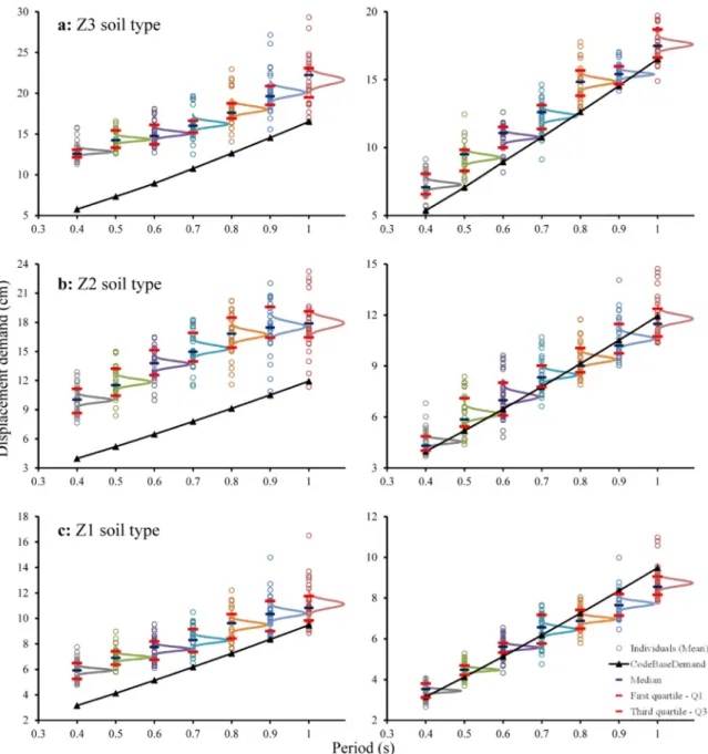
Fig. 11. Distribution of displacement demands according to nonlinear static and dynamic procedures (Left: Fy/W = 0.1, Right: Fy/W = 0.3).

y = 10.66x + 2.51 ρ = 0.99 y = 8.69x + 1.44_{ρ = 0.98} y = 9.43x + 0.36 ρ = 0.98 0 2 4 6 8 10 12 14 0.3 0.4 0.5 0.6 0.7 0.8 0.9 1.0 1.1 Displa ce m ent de m an d (c m )

Fy/W=0.1 Fy/W=0.2 Fy/W=0.3

y = 16.57x + 5.71 ρ = 0.98 y = 16.74x + 0.70 ρ = 1.00 y = 12.46x + 0.98 ρ = 0.99 0 5 10 15 20 25 0.3 0.4 0.5 0.6 0.7 0.8 0.9 1.0 1.1 Period (s) y = 18.61x + 6.29 ρ = 0.98 y = 15.60x + 4.41 ρ = 0.97 y = 17.09x + 1.97 ρ = 0.98 0 5 10 15 20 25 30 0.3 0.4 0.5 0.6 0.7 0.8 0.9 1.0 1.1

(10)

μ are calculated using Eq.(12). InTable 4, 95% confidence intervals (L, U) of mean of the populations are given. For instance, considering the SDOF system with T = 0.40s and Fy/W = 0.10, 95% confidence interval of μ is 5.65–6.21cm for soil Z1. Hence, it can be said that the resultant interval indeed contains μ with confidence 95%. Considering the same SDOF system, 95% confidence interval of μ is 9.49–10.50cm for soil Z2, and 12.43–13.23cm for soil Z3. For the other SDOF systems considered in this study, 95% confidence interval can also be shown inTable 4.

5. Reliability-based demand estimation and comparison of code procedures

It was argued with ANOVA and sampling distributions that seismic displacement demands obtained for the ground motion record sets compatible with the same design spectrum are randomly selected samples from the same population and possibility of demand ranges for each fundamental period and lateral strength ratios was determined.

In addition to nonlinear dynamic analysis procedures, nonlinear static procedures are also suggested in code based applications con-sidering the same seismic hazard levels to perform fast approximation of seismic demand for performance evaluation purposes. Code con-formed static procedures, on the other hand, with minor differences use the similar approaches and they generally require the identification of capacity curve and natural period of the structure[19,22,43,44]. Al-though nonlinear dynamic analysis technique is more reliable method to determine demands and structural behavior of the buildings, static procedures can also be used for preliminary assessment and foresee the seismic demands. But, unlike static procedures, estimations of nonlinear dynamic analyses are variable even for the same seismic hazard as the behavior of structure is completely affected from the characteristics of earthquakes. For this reason, seismic demands of static procedure of the considered code are determined in addition to dynamic analysis results. By this way, the use of both methods in seismic codes is compared and some important implications and recommendations are given for the practitioners in the field.

In Fig. 11, demand estimation of static and dynamic results is plotted for each lateral strength ratio, fundamental period and soil classes. For evaluation, some descriptive statistics like mean, median and first and third quartile of the dynamic analysis results are also determined. In the figure, probability distribution of dynamic analysis results is also given according to fundamental period of the structure considering the 95% confidence level previously determined inSection 4.3. It can be seen from the figure that static procedure approximations are increasing with an increasing period and even it may result in higher than dynamic results from Z3 to Z1 especially at high lateral strength ratios (Fy/W = 0.3). Furthermore, static procedure estimations get closer to dynamic results at long structural periods and stiff soils. This situation implies that special attention should be made to non-linear static procedure estimations for buildings with high periods. Nevertheless, it can be accepted that in general, dynamic analysis give more conservative results compared to static one.

A generally accepted view in the seismic codes is that if more than seven records are used, mean of structural responses are used for the constructed record set. However, if one uses, more than one record set that compatible to considered target response spectrum (seismic ha-zard) then which of the descriptive statics should be used for the per-formance evaluation? This arising question also becomes clear from the illustrations of theFig. 11and the figure clearly manifests that mean and median values of the record sets are almost identical. In other words, results show that both statistical measures can be used, but the means of the records are still slightly conservative compared to median one. It is also worth noting that the means can be affected from outliers. The first and third quartile of dynamic analysis results has also re-vealed a very striking finding in comparison of seismic demand esti-mation of dynamic analysis results. It can be inferred from the figures that first and third quartile of the individual means of records range

between lower and upper confidence limits that are determined from the sampling distribution of dynamic analysis result with 95% con-fidence level and this finding is also valid for each soil class and lateral strength ratios. In addition, it was observed that average of first and third quartile values are very close the mean of individual mean of records sets. When the proportion of these values (average of quartiles and individual mean of records sets) are calculated, it was determined that the ratio is 1.01 and the lowest and highest values were obtained as 0.98 and 1.03, respectively.

Considering the sampling distribution of the mean displacements and overall statistical assessments on the seismic demands, reliability based demand estimations can be performed for different structures represented by equivalent SDOF systems. For this purpose, 10% ex-ceedance probability of displacement demands are estimated for all SDOF systems considering all the record sets used in this study. Furthermore, linear regression analysis was performed to investigate correlation between fundamental period and seismic demands for each soil class and lateral strength ratio. Calculated correlation coefficient between period and displacement demand have shown the good agreement as can be seen form theFig. 12.

In the figure, equations of the linear curves are also given depending on the fundamental periods for each lateral strength ratio and soil type. Observed high correlations show that derived equations can be used for rapid prediction of seismic demands in reliability based manner. In other words, predicted demands have 10% exceedance probability and it can be said that one may predict the seismic demands very simply with very low risk (10% probability) without performing any nonlinear time history analysis and/or statistical assessment by only using the fundamental period of the structure.

6. Results

In this study, maximum displacement demands of SDOF systems obtained from nonlinear time history analysis using different real ground motion record sets compatible with TEC are statistically eval-uated. In order to consider the broad range of SDOF systems, vibration period and lateral strength ratio for SDOF systems are selected between 0.4 s–1.0 s and 0.1–0.3, respectively. 30 ground motion record sets compatible with elastic design spectra defined for each local soil classes Z1, Z2 and Z3 in TEC are used for the analyses. Totally, 13,230 non-linear time history analysis (21 SDOF systems and 90 ground motion record sets each of them has seven ground motion records) are per-formed. Performing nonlinear time history analysis of the SDOF sys-tems, maximum displacement demands are calculated for each of the ground motion records in the record sets. Then, the mean of maximum displacement demands are calculated for each of the record sets, se-parately. In order to evaluate the dispersion of the maximum dis-placement demands obtained from ground motion records around the mean of the sets, coefficient of variation values are calculated. The significance of the difference between the mean displacement demands calculated for different ground motion record sets is also evaluated using one-way ANOVA. In addition, confidence intervals are calculated for mean displacement demands for each SDOF system and local soil class considered in this study. Finally, linear regression models are proposed to estimate seismic displacement demands of the SDOF sys-tems for a certain value of exceedance probability. The results of the study could be summarized as follows:

a) In modern seismic design codes, ground motion selection procedures for time history analysis only consider the mean spectrum of the se-lected ground motions and target design spectrum without con-sidering random variability of the ground motion records. Thus, the variation of the seismic demands of SDOF systems obtained using code-compatible ground motion record sets is generally high. This variation may be considered for detailed probabilistic seismic per-formance assessment and/or seismic design of a specific structure.

(11)

b) The mean displacement demands calculated for a SDOF system using different ground motion record sets may differ although the record sets are compatible with the same design spectrum. Therefore, mean displacement demands can be accepted as random variables which change depending on the code-compatible record sets used for time history analysis.

c) According to one-way ANOVA results, the variance of the maximum displacement demands obtained from the individual ground motion records in the sets due to random causes is quite larger than the variance due to the differences between the mean displacement demands of the record sets compatible with the same design spec-trum. Hence, the differences between the mean displacement de-mands of ground motion record sets can be accepted as statistically insignificant at significance level α = 0.05. In other words, max-imum displacement demands in ground motion record sets can be accepted as simply random samples drawn from the same popula-tion at 90% confidence level.

d) The abovementioned results are valid for all the SDOF systems and local soil classes considered in this study.

e) Considering one-way ANOVA results, it is possible to make in-ferences about unknown parameters of the distribution of the po-pulations. In order to do this, statistics can be calculated evaluating the nonlinear analyses results using the large number of ground motion record sets. For example, confidence interval can be esti-mated for the population mean at the desired level of confidence. In this circumstance, confidence interval at selected 95% level of confidence for the population means are also estimated using levant maximum displacement demands of 30 ground motion re-cords as random samples, separately, for each of the SDOF systems and local soil classes used in this study.

f) Mean and median values of the seismic displacement demands ob-tained for the different record sets compatible with the same design spectrum are almost identical. Therefore, both statistical measures can be used for seismic design or performance evaluation if more than one ground motion records are used for time history analysis. But, it is also worth noting that means of the demands are still slightly conservative compared to median of the demands. g) Using sampling distribution of the populations of mean

displace-ment demands, it is also possible to perform reliability based de-mand estimation for different structures represented by equivalent SDOF systems. In this study, the mean displacement demands of ground motion record sets for 10% exceedance probability are cal-culated for each SDOF system and local soil class considered in this study. Then, linear regression models, depending on the funda-mental periods for each lateral strength ratio and soil type, are

proposed for rapid prediction of displacement demands in reliability based manner. Predicted demands have 10% exceedance probability and it can be said that one may predict the demands very simply with very low risk (10% probability) without performing any non-linear time history analysis and/or statistical assessment by only using the fundamental period and lateral strength ratio of the structure.

In this study, TEC compatible ground motion record sets are used to perform nonlinear time history analyses. Thus, the results are valid for TEC and considered hazard zonation map. In the near future, the new seismic code TBEC[45], and new hazard zonation map (https://tdth. afad.gov.tr) will be effective in Turkey. It should be noted that many of modern seismic codes (FEMA-368[18]; EUROCODE-8[19]; ASCE 07-05[20]; GB[21]), including TBEC, describe relatively similar proce-dures with TEC in terms of requiring spectral matching between the design spectrum and the response spectrum of a selected record set within a stated period range. Thus, it can be said that similar results of this study are obtained when the ground motion record sets compatible with the abovementioned seismic design codes are used for nonlinear time history analyses. Hence, using code-compatible different ground motion sets for nonlinear time history analyses of a structure it is possible to obtain information about the distribution of the population of the seismic demands which are used for design or assessment of that structure according to modern seismic codes.

Based on these results, it can be stated that there is a significant requirement for the consideration of variability in structural responses, numerically. For instance, reducing the variation of maximum dis-placement demands in the record sets may become a matter in future studies. In order to this, not only mean spectra of the record sets but also individual spectra of ground motion records in the record sets may be considered for compatibility with the target spectra. In addition, using two or three-dimensional structural models to perform code-based nonlinear time history analysis would provide remarkable results for evaluating the various seismic response parameters such as; global drift ratio, interstory drift ratio, internal forces or ductility demands etc. Different type of structures such as mid- or high-rise buildings, bridges etc., which have their fundamental periods are longer than 1.0 s, would also be considered. Probability based approaches may also become the future direction of taking the variability of structural responses into consideration numerically. The FEMA P-58 methodology[46]can be used to assess the probable seismic performance of buildings for par-ticular earthquake scenario intensity, or considering all earthquakes that could occur, and the likelihood of each, over a specified period of time.

Appendix A

See AppendixTables A1–A3

Table A1

Ground motion record sets obtained for Soil Z1.

Set 1 Set 2 Set 3 Set 4 Set 5 Set 6

Record Scale Record Scale Record Scale Record Scale Record Scale Record Scale

5270-Y 1.014 646-Y 0.816 5272-Y 1.440 6272-X 1.848 6331-X 0.671 6272-X 1.961

410-X 1.782 383-Y 1.449 6331-X 1.132 5272-Y 1.698 467-X 1.317 6262-Y 0.778

292-X 1.344 362-X 1.475 382-X 1.448 6327-Y 1.151 410-X 2.000 603-Y 1.967

362-X 1.554 292-X 0.971 5655-X 0.787 605-X 0.924 243-X 1.834 6269-Y 0.621

7158-X 0.632 1243-X 0.789 6270-Y 0.894 368-X 0.851 6278-X 0.511 6267-X 1.818

6272-Y 1.224 5272-Y 1.664 292-X 0.818 383-Y 0.993 960-X 1.104 598-Y 1.965

6327-Y 0.519 6331-X 1.166 362-Y 0.972 467-Y 1.277 5272-Y 0.669 6100-X 1.565

6269-Y 0.576 6331-Y 1.493 369-X 1.058 6272-Y 1.590 6100-Y 1.140 647-X 1.574

368-Y 0.878 646-Y 0.891 292-X 1.751 467-X 1.012 467-X 1.196 412-X 1.322

(12)

Table A1 (continued)

6337-X 1.772 1891-Y 0.545 410-Y 0.604 369-Y 0.723 1891-Y 1.854 410-X 0.953

6272-Y 1.399 4557-X 1.413 1891-Y 1.517 6262-X 1.054 6341-X 0.846 6331-X 0.841

604-X 1.829 292-Y 1.361 140-Y 0.590 646-X 0.872 5272-X 1.854 598-Y 1.077

6331-Y 1.732 6269-Y 1.492 6267-Y 1.261 292-Y 1.002 292-Y 0.983 467-Y 1.933

6262-X 0.781 6262-X 0.545 4679-Y 0.553 6337-X 1.486 646-Y 1.272 292-X 1.209

6761-X 0.725 1891-Y 1.262 6265-Y 0.847 6341-X 0.503 5272-Y 1.773 646-Y 1.247

6333-Y 0.522 1243-X 0.868 6326-Y 0.646 647-X 2.000 6336-Y 1.281 6269-Y 1.125

234-Y 0.748 628-X 0.500 5270-Y 1.280 369-X 1.002 5270-Y 1.418 467-Y 1.305

5272-Y 1.970 6278-Y 0.840 357-Y 1.997 292-X 1.116 410-Y 1.022 292-X 0.668

1891-Y 1.465 5271-X 2.000 369-X 0.903 603-Y 1.999 357-Y 0.826 369-X 1.934

243-X 1.702 412-X 1.584 603-Y 1.340 6327-Y 1.027 603-Y 1.809 6333-X 1.663

638-Y 1.190 6331-X 1.207 6327-Y 0.794 605-X 1.088 234-Y 0.667 382-X 1.068

960-Y 1.285 359-Y 0.508 604-X 1.918 292-Y 1.269 6270-X 0.987 1243-X 1.265

1891-Y 1.058 243-X 1.985 410-X 1.384 362-Y 0.897 385-Y 0.580 6272-Y 1.668

6331-Y 0.978 4679-Y 0.743 629-Y 0.579 598-X 0.978 5272-Y 1.728 6337-X 1.097

368-Y 0.840 6100-X 1.112 6327-Y 1.149 6333-X 1.889 369-Y 1.002 646-Y 1.459

6262-Y 0.801 292-X 1.240 605-X 1.554 646-Y 1.217 410-X 1.038 5272-Y 1.523

6333-X 1.202 5272-Y 0.921 6333-X 1.992 5272-Y 1.622 6336-Y 1.364 243-Y 1.954

383-Y 1.747 6331-X 1.270 6331-Y 1.230 6270-Y 1.307 4678-Y 0.688 598-X 1.063

368-Y 1.191 357-Y 1.999 639-X 1.084 6267-X 0.992 4678-X 0.539 641-X 0.935

603-Y 1.780 642-Y 0.936 960-Y 0.570 646-Y 1.523 5271-X 1.998 604-Y 1.095

292-Y 0.635 5270-Y 0.673 412-X 1.318 410-Y 1.183 960-X 0.683 646-Y 1.510

243-X 1.238 6272-Y 1.895 6262-Y 0.987 467-Y 1.172 6278-Y 0.993 6337-X 1.760

6327-Y 0.905 292-Y 0.501 6333-X 1.430 385-X 1.116 6331-X 0.928 6270-Y 1.313

6331-Y 1.425 5272-Y 1.523 604-X 1.932 243-Y 1.264 410-X 0.781 292-Y 1.138

6333-X 1.477 467-Y 1.759 642-X 0.674 6262-Y 0.788 6272-X 1.161 5272-Y 1.403

Table A2

645-Y 1.394 1859-X 0.992 6496-Y 1.721 6447-Y 1.919 572-Y 1.626 352-Y 1.167

352-Y 1.275 946-Y 1.786 1735-X 0.835 352-Y 0.592 759-Y 0.673 7155-Y 1.219

548-X 0.711 6496-Y 1.803 532-Y 1.061 232-Y 1.273 1859-X 0.630 645-Y 0.861

6422-X 1.600 645-Y 1.182 595-X 0.910 142-Y 1.023 645-Y 1.592 630-Y 0.775

946-Y 0.903 1720-Y 0.636 760-X 0.870 760-X 1.054 352-Y 1.239 946-Y 0.764

760-Y 1.467 595-X 0.819 142-Y 1.523 1735-X 1.688 7161-X 0.925 572-X 1.514

572-Y 1.747 142-Y 1.501 352-Y 0.982 6496-Y 1.309 6144-X 1.093 6138-Y 1.103

1984-X 0.715 6138-X 1.125 1711-X 0.745 761-Y 0.628 1984-X 1.899 352-Y 0.782

1881-Y 0.963 760-X 0.826 532-Y 0.975 1859-X 0.832 129-Y 0.875 1735-X 0.719

1735-Y 0.606 352-Y 1.333 142-Y 1.196 595-X 1.093 611-Y 0.518 232-X 0.980

6447-Y 1.995 620-X 0.787 352-Y 0.884 759-X 0.781 6138-X 1.958 572-X 0.765

612-X 0.614 232-X 0.736 548-X 0.511 6142-Y 0.817 142-Y 1.021 6138-Y 1.402

129-X 1.221 548-X 0.992 6138-X 1.136 502-Y 0.770 1859-X 1.830 759-X 1.195

572-X 1.378 549-Y 0.807 946-X 1.770 946-Y 1.713 49-Y 0.522 142-Y 0.974

572-X 1.093 6144-Y 0.685 352-Y 1.058 760-X 1.541 7155-Y 0.974 7067-X 1.948

611-Y 0.861 1859-X 1.684 5798-Y 0.876 572-Y 0.689 6494-Y 0.667 6145-X 1.211

6447-Y 1.498 1996-X 0.993 620-Y 0.839 6499-X 1.028 6138-Y 1.018 1720-X 1.552

5813-X 0.919 1720-X 1.341 1996-X 1.712 595-X 0.922 1881-X 0.749 760-X 0.707

6142-Y 0.803 352-Y 1.497 129-X 1.267 532-Y 1.197 569-Y 0.748 572-Y 1.086

595-X 0.510 645-Y 1.074 1720-X 1.477 620-Y 0.517 6142-Y 0.604 142-X 1.377

352-Y 0.921 572-Y 0.720 5813-Y 0.868 352-Y 1.560 572-X 1.393 352-Y 1.420

502-X 1.026 532-Y 0.791 6329-Y 1.083 572-Y 1.189 532-Y 1.300 244-Y 1.180

645-Y 0.681 6496-Y 1.670 946-Y 1.096 244-Y 1.787 946-X 1.437 129-X 1.415

1720-X 0.958 49-Y 0.500 6494-Y 1.274 352-Y 1.072 6138-Y 1.472 1881-Y 0.543

232-X 1.064 142-Y 0.936 645-Y 1.597 502-X 0.926 474-Y 0.994 502-Y 1.953

760-X 1.080 352-Y 0.850 1859-X 1.411 142-Y 1.119 129-X 0.741 6138-Y 1.574

(13)

Table A2 (continued)

352-Y 1.212 645-Y 1.103 1996-X 0.779 6138-Y 1.111 352-Y 0.828 1735-Y 0.975

142-Y 1.326 232-X 0.942 5798-Y 0.776 1881-Y 0.780 142-Y 1.115 142-Y 1.438

6138-X 1.120 572-Y 0.961 530-Y 0.520 142-Y 1.408 474-Y 0.661 6447-Y 1.578

5798-Y 1.283 6494-Y 0.838 244-Y 1.280 7067-X 1.874 352-Y 0.870 1720-X 0.792

946-Y 1.221 946-Y 1.161 7067-X 1.736 6144-X 1.165 759-X 1.014 572-X 0.965

759-X 0.798 211-Y 0.622 6142-Y 0.716 6447-X 1.903 6138-Y 1.266 352-Y 0.910

6142-Y 0.637 7161-X 1.351 352-Y 0.610 760-Y 1.352 142-Y 1.426 6142-Y 0.660

129-X 1.163 612-X 0.519 761-Y 0.740 232-X 1.127 7067-X 1.642 244-Y 1.876

1735-X 1.167 474-X 0.997 7257-X 1.344 352-Y 1.192 232-X 1.106 5813-X 0.783

Table A3

360-X 0.704 601-Y 1.008 141-X 1.988 6962-X 1.998 7010-Y 1.084 6962-Y 1.998

374-Y 0.672 648-Y 0.743 151-X 0.923 7104-X 0.728 1230-Y 0.617 360-X 0.591

602-X 0.999 360-X 0.831 7010-X 1.378 375-Y 0.904 141-Y 1.161 141-X 1.993

6962-Y 1.355 6606-Y 1.105 1230-X 0.540 1230-X 0.693 6975-Y 0.917 6978-Y 0.700

6978-Y 0.622 1230-X 0.548 6606-Y 1.301 360-X 1.044 151-X 0.597 6606-Y 1.463

6606-Y 0.582 6975-Y 1.096 6978-Y 0.819 6978-Y 0.757 602-X 0.717 1230-X 0.546

1230-X 0.788 375-Y 0.600 6962-Y 1.984 7010-Y 1.913 643-X 1.340 151-X 0.916

6606-Y 0.664 375-Y 0.604 1959-Y 1.914 1230-X 0.766 7010-X 1.838 7104-Y 0.581

439-Y 0.553 6962-Y 0.932 6975-Y 0.867 602-X 0.816 1230-X 0.501 1230-X 0.540

6975-Y 0.779 602-X 0.834 360-X 0.658 7104-Y 0.645 6975-Y 0.965 141-X 1.927

1230-X 0.660 360-X 0.839 7010-Y 1.083 375-Y 0.655 648-Y 0.532 648-X 0.615

633-X 1.468 1230-X 0.799 601-Y 1.185 360-X 0.919 141-X 2.000 151-X 0.761

360-X 0.669 6606-Y 0.692 1230-Y 0.618 6975-Y 0.579 6606-Y 1.323 6978-Y 1.036

141-X 1.190 6978-Y 0.769 375-Y 0.625 7010-Y 1.057 151-X 0.812 6962-Y 1.548

1908-X 0.673 6975-Y 0.679 375-Y 0.743 1230-Y 0.572 1230-Y 0.528 375-Y 0.645

6975-Y 0.622 7010-Y 1.193 6606-Y 0.626 151-X 0.752 6962-X 1.988 6606-Y 1.073

602-X 1.082 1230-X 0.740 6978-Y 0.718 6975-Y 0.856 6978-Y 0.803 141-X 1.725

360-X 0.814 360-X 0.848 6962-X 1.808 7010-X 1.808 141-X 1.642 6978-Y 1.165

6606-Y 0.934 375-Y 0.619 1230-X 0.755 6963-Y 0.503 151-X 1.183 7010-Y 0.742

374-Y 0.619 602-X 0.835 602-X 0.791 141-Y 1.142 7010-X 0.832 360-X 0.798

1230-X 0.709 6606-Y 0.890 360-X 0.830 602-X 0.655 6963-Y 0.881 1230-X 0.773

1230-X 0.505 6975-Y 0.915 6978-Y 0.666 7010-X 1.690 360-X 0.674 6978-Y 0.525

151-X 1.015 1230-X 0.543 602-X 0.869 601-Y 0.995 6606-Y 1.566 375-Y 0.539

1908-X 0.962 602-X 0.742 6962-Y 1.632 1230-Y 0.572 6975-Y 0.716 1230-X 0.820

141-X 1.999 648-Y 0.655 360-X 0.849 1959-Y 1.860 141-X 1.255 6962-Y 1.464

6962-Y 1.421 151-X 0.593 6606-Y 0.728 6975-Y 0.897 602-X 0.873 360-X 0.862

6606-Y 1.077 360-X 0.572 1230-X 0.699 360-X 0.708 374-Y 0.544 602-X 0.958

6978-Y 1.026 6606-Y 1.024 374-Y 0.652 375-Y 0.693 1230-X 0.663 6606-Y 0.628

374-Y 0.530 1230-X 0.762 6975-Y 0.706 7010-Y 1.470 360-X 0.981 375-Y 0.648

6606-Y 1.119 6978-Y 1.108 1230-X 0.737 151-X 0.548 7010-Y 1.797 6606-Y 1.183

6975-Y 0.651 375-Y 0.649 648-Y 0.571 1908-X 1.490 6962-Y 0.869 141-X 1.281

1230-X 0.727 360-Y 0.852 7010-Y 1.117 602-X 0.788 1230-X 0.577 360-X 0.949

1908-X 1.064 141-X 0.502 360-X 0.779 6975-Y 0.848 648-X 0.662 6978-Y 1.240

602-X 0.930 602-X 0.609 602-X 0.684 379-Y 0.547 555-Y 1.937 950-X 0.539

(14)

Appendix B

See AppendixTable B1

Table B1

Detailed information about selected ground motion records for the record sets.

Record Earthquake Name Date M Station Record Earthquake Name Date M Station

49 Friuli 06/05/76 6.5 ST14 530 Racha (aftershock) 15/06/91 6.0 ST200

129 Friuli (aftershock) 15/09/76 6.0 ST14 532 Racha (aftershock) 15/06/91 6.0 ST202

140 Friuli (aftershock) 15/09/76 6.0 ST36 548 Izmir 06/11/92 6.0 ST43

141 Friuli (aftershock) 15/09/76 6.0 ST12 549 Izmir 06/11/92 6.0 ST162

142 Friuli (aftershock) 15/09/76 6.0 ST14 555 Kallithea 18/03/93 5.8 ST10

151 Friuli (aftershock) 15/09/76 6.0 ST33 569 Patras 14/07/93 5.6 ST166

211 Montenegro (aftershock) 15/04/79 5.8 ST67 572 Patras 14/07/93 5.6 ST178

232 Montenegro (aftershock) 24/05/79 6.2 ST77 595 Umbria Marche 26/09/97 5.7 ST83

234 Montenegro (aftershock) 24/05/79 5.8 ST68 598 Umbria Marche 26/09/97 6.0 ST222

243 Valnerina 19/09/79 5.8 ST82 601 Umbria Marche 26/09/97 5.7 ST224

244 Valnerina 19/09/79 5.8 ST83 602 Umbria Marche 26/09/97 6.0 ST224

292 Campano Lucano 23/11/80 6.9 ST98 603 Umbria Marche 26/09/97 5.7 ST225

352 Biga 05/07/83 6.1 ST131 604 Umbria Marche 26/09/97 6.0 ST225

357 Umbria 29/04/84 5.6 ST134 605 Umbria Marche 26/09/97 5.7 ST84

362 Umbria 29/04/84 5.6 ST137 620 Umbria Marche (aftershock) 06/10/97 5.5 ST83

368 Lazio Abruzzo 07/05/84 5.9 ST143 628 Umbria Marche (aftershock) 06/10/97 5.5 ST226 369 Lazio Abruzzo 07/05/84 5.9 ST109 629 Umbria Marche (aftershock) 06/10/97 5.5 ST225 374 Lazio Abruzzo 07/05/84 5.9 ST148 630 Umbria Marche (aftershock) 06/10/97 5.5 ST228 375 Lazio Abruzzo 07/05/84 5.9 ST149 633 Umbria Marche (aftershock) 14/10/97 5.6 ST227 379 Lazio Abruzzo (aftershock) 11/05/84 5.5 ST1034 638 Umbria Marche (aftershock) 14/10/97 5.6 ST233 382 Lazio Abruzzo (aftershock) 11/05/84 5.5 ST140 639 Umbria Marche (aftershock) 14/10/97 5.6 ST226 383 Lazio Abruzzo (aftershock) 11/05/84 5.5 ST153 641 Umbria Marche (aftershock) 14/10/97 5.6 ST84 385 Lazio Abruzzo (aftershock) 11/05/84 5.5 ST155 642 Umbria Marche (aftershock) 14/10/97 5.6 ST225

410 Golbasi 05/05/86 6.0 ST161 643 Umbria Marche (aftershock) 14/10/97 5.6 ST224

412 Golbasi 06/06/86 5.8 ST161 645 Umbria Marche (aftershock) 14/10/97 5.6 ST83

439 Spitak 07/12/88 6.7 ST173 646 Umbria Marche (aftershock) 14/10/97 5.6 ST234

467 Chenoua 29/10/89 5.9 ST181 647 Umbria Marche (aftershock) 14/10/97 5.6 ST222

474 Filippias 16/06/90 5.5 ST123 648 Umbria Marche (aftershock) 14/10/97 5.6 ST221

502 Racha (aftershock) 03/05/91 5.6 ST200 759 Umbria Marche 26/09/97 5.7 ST265

760 Umbria Marche 26/09/97 6.0 ST265 6262 South Iceland 17/06/00 6.5 ST2496

761 Umbria Marche (aftershock) 14/10/97 5.6 ST265 6265 South Iceland 17/06/00 6.5 ST2494

946 Potenza 05/05/90 5.8 ST103 6267 South Iceland 17/06/00 6.5 ST2565

950 Sicilia-Orientale 13/12/90 5.6 ST288 6269 South Iceland 17/06/00 6.5 ST2497

960 Sicilia-Orientale 13/12/90 5.6 ST296 6270 South Iceland 17/06/00 6.5 ST2556

1230 Izmit 17/08/99 7.6 ST576 6272 South Iceland 17/06/00 6.5 ST2568

1243 Izmit (aftershock) 13/09/99 5.8 ST575 6278 South Iceland 17/06/00 6.5 ST2552

1711 Ano Liosia 07/09/99 6.0 ST1255 6326 South Iceland (aftershock) 21/06/00 6.4 ST2496

1720 Dinar 01/10/95 6.4 ST543 6327 South Iceland (aftershock) 21/06/00 6.4 ST2552

1735 Adana 27/06/98 5.7 ST581 6329 South Iceland (aftershock) 21/06/00 6.4 ST2485

1859 Near NW coast of Kefallinia island 27/02/87 5.7 ST1303 6331 South Iceland (aftershock) 21/06/00 6.4 ST2486 1881 South Aegean 23/05/94 6.1 ST1310 6333 South Iceland (aftershock) 21/06/00 6.4 ST2487 1891 Kranidia 25/10/84 5.5 ST1320 6336 South Iceland (aftershock) 21/06/00 6.4 ST2563 1908 Filippias 16/06/90 5.5 ST126 6337 South Iceland (aftershock) 21/06/00 6.4 ST2494 1959 Kyllini 16/10/88 5.9 ST214 6341 South Iceland (aftershock) 21/06/00 6.4 ST2497 1984 Kefallinia island 23/01/92 5.6 ST1353 6422 Izmit (aftershock) 13/09/99 5.8 ST3135

1996 Anchialos 30/04/85 5.6 ST1355 6447 Izmit (aftershock) 11/11/99 5.6 ST3140

4557 Bovec 12/04/98 5.7 ST750 6494 Duzce 1 12/11/99 7.2 ST3134

4678 South Iceland 17/06/00 6.5 ST2557 6606 Izmit (aftershock) 11/11/99 5.6 ST2571

4679 South Iceland 17/06/00 6.5 ST2563 6761 Vrancea 30/08/86 7.2 ST40

5270 Mt. Vatnafjoll 25/05/87 6.0 ST2486 6962 Izmit (aftershock) 13/09/99 5.8 ST3271 5271 Mt. Vatnafjoll 25/05/87 6.0 ST2483 6963 Izmit (aftershock) 13/09/99 5.8 ST3268 5272 Mt. Vatnafjoll 25/05/87 6.0 ST2487 6975 Izmit (aftershock) 13/09/99 5.8 ST3272 5655 NE of Banja Luka 13/08/81 5.7 ST2950 6978 Izmit (aftershock) 13/09/99 5.8 ST3273 5798 Gulf of Akaba (aftershock) 23/11/95 5.6 ST2989 7010 Izmit (aftershock) 11/11/99 5.6 ST772

5813 Itea 05/11/97 5.6 ST857 7067 Altinsac 15/11/00 5.5 ST608

6100 Kozani 13/05/95 6.5 ST1315 7104 Ishakli (aftershock) 03/02/02 5.8 ST856

6138 Aigion 15/06/95 6.5 ST1330 7155 Firuzabad 20/06/94 5.9 ST3290

(15)

Appendix C

See AppendixTables C1–C6

Table C1

mΔvalues for all the SDOF systems and ground motion record sets for Soil Z1 (cm).

T (s) 0.40 0.50 0.60 0.70 0.80 0.90 1.00 Fy/W 0.10 0.20 0.30 0.10 0.20 0.30 0.10 0.20 0.30 0.10 0.20 0.30 0.10 0.20 0.30 0.10 0.20 0.30 0.10 0.20 0.30 Set1 5.13 3.54 3.83 6.49 5.20 4.48 7.92 5.46 5.71 7.76 6.00 6.54 7.64 7.85 7.16 8.46 8.35 7.72 8.86 7.95 8.20 Set2 5.63 4.37 4.07 6.68 4.67 4.39 8.53 5.63 5.55 9.67 6.26 7.17 11.02 7.05 7.40 10.65 7.60 7.15 10.88 8.34 7.96 Set3 5.37 4.45 3.83 6.91 4.85 4.27 7.71 5.87 6.38 9.42 6.39 7.20 10.81 6.76 7.36 10.70 7.59 7.89 10.51 8.39 8.17 Set4 6.73 4.30 2.81 6.92 5.38 3.98 7.06 6.66 6.07 7.21 6.67 5.38 8.15 6.89 6.84 9.52 7.50 7.58 11.34 9.47 8.53 Set5 5.24 3.75 3.03 5.84 5.42 4.58 6.28 5.46 5.62 6.84 6.24 6.11 7.69 7.59 7.50 8.94 9.70 8.54 9.56 9.02 9.26 Set6 5.94 3.59 2.66 6.70 4.27 4.22 7.09 6.19 5.74 7.43 7.87 6.22 8.38 8.04 6.59 9.67 9.06 7.98 10.54 9.73 10.80 Set7 5.90 3.73 3.65 7.55 4.67 4.49 9.15 6.02 5.36 9.83 6.26 5.94 11.37 7.03 6.88 11.43 8.55 8.29 13.00 10.47 9.14 Set8 6.83 4.75 3.85 8.09 7.09 4.50 8.41 7.03 5.42 9.40 6.81 7.05 11.46 6.46 6.56 11.69 7.91 7.43 11.56 9.00 8.16 Set9 4.96 3.35 3.64 6.12 5.97 4.80 6.80 6.49 5.75 8.46 8.69 7.26 8.44 8.80 7.94 9.00 7.99 6.96 11.46 9.43 8.66 Set10 5.04 3.73 3.80 7.40 4.91 4.26 7.43 5.55 4.96 7.10 6.60 5.74 9.64 6.73 6.63 11.18 6.41 7.91 10.87 8.60 8.33 Set11 6.63 4.33 3.69 8.98 6.19 4.66 8.27 6.71 5.69 8.09 8.35 6.80 9.80 8.59 7.42 11.39 9.24 8.77 12.61 10.08 9.55 Set12 5.06 3.77 3.63 6.57 5.47 4.94 7.98 6.79 6.54 8.88 8.44 7.59 9.15 8.49 7.76 10.27 7.77 8.39 10.32 8.04 8.48 Set13 6.11 4.82 3.68 7.34 5.62 4.68 7.95 6.60 5.94 8.65 5.97 5.42 9.00 6.52 5.99 8.67 7.11 7.11 9.83 8.10 7.83 Set14 5.26 3.86 3.28 6.64 4.15 4.53 7.84 5.00 4.72 8.75 6.24 7.39 9.90 8.29 7.60 10.10 9.12 8.18 10.81 9.52 8.93 Set15 7.75 3.74 2.96 8.45 4.31 4.42 9.54 5.11 4.67 10.50 6.45 4.76 10.85 6.99 7.25 12.23 7.75 6.92 13.21 8.58 8.03 Set16 5.99 3.36 3.20 7.00 4.88 4.12 7.93 5.30 5.33 8.78 7.66 5.79 9.95 7.38 6.95 10.71 7.30 7.38 11.53 8.81 8.84 Set17 6.45 4.41 4.05 6.15 4.89 4.67 6.66 5.98 6.00 6.87 7.29 6.77 8.05 6.23 6.42 9.01 6.88 7.25 10.45 7.59 7.84 Set18 6.81 4.16 3.25 8.05 5.31 5.10 7.75 6.37 5.13 8.52 6.84 7.22 9.17 6.83 6.51 9.97 8.10 6.46 10.72 8.13 8.56 Set19 5.98 4.00 2.99 6.90 5.24 5.29 6.51 6.83 5.32 7.21 6.58 5.69 8.42 7.16 6.48 10.30 9.30 7.90 10.71 9.38 10.57 Set20 5.59 4.01 3.89 7.18 5.08 4.41 9.02 4.97 5.73 9.74 6.95 7.66 9.89 7.27 7.42 10.40 7.46 7.27 9.84 9.08 8.26 Set21 7.34 3.87 3.34 7.42 5.02 3.96 8.18 4.97 5.07 9.47 6.14 5.94 12.20 7.36 7.11 14.79 9.67 8.29 16.51 10.37 8.33 Set22 7.07 4.44 3.44 7.48 6.40 4.24 7.81 6.39 5.54 8.43 7.28 6.75 10.84 6.96 6.40 12.71 8.47 7.12 13.70 8.14 7.91 Set23 5.65 3.72 3.48 6.48 4.75 3.86 6.94 5.42 5.59 7.50 6.04 6.11 9.80 7.03 6.88 11.74 7.68 6.97 12.34 8.39 8.40 Set24 5.58 3.64 3.14 6.37 4.14 3.70 7.34 5.03 4.34 8.06 6.31 5.23 9.62 6.90 6.18 8.99 7.17 7.73 9.09 8.59 8.57 Set25 5.60 3.76 3.14 6.16 5.33 4.48 6.56 5.21 6.24 7.47 6.23 6.26 9.63 6.02 6.63 11.38 7.97 7.72 13.35 9.16 9.32 Set26 4.77 3.65 3.58 5.79 4.98 5.02 6.35 5.82 5.48 7.50 5.86 5.47 8.50 6.57 5.79 8.83 7.69 7.01 9.14 9.76 9.03 Set27 5.96 3.65 3.12 6.98 4.51 4.23 7.77 5.77 5.69 8.16 7.56 7.09 9.00 8.65 8.05 10.42 10.30 9.99 10.93 10.17 10.98 Set28 6.40 4.42 3.59 6.37 5.42 5.12 6.12 6.74 6.29 6.48 7.73 7.39 7.61 7.53 6.86 8.36 8.70 7.58 9.35 8.98 8.83 Set29 4.88 3.37 2.90 6.09 4.58 4.75 6.52 6.13 5.51 7.11 6.53 6.91 8.65 6.96 7.90 9.79 7.74 8.39 9.64 9.45 8.75 Set30 6.26 4.65 3.86 7.46 5.84 4.08 8.66 6.70 5.66 9.08 7.46 6.59 10.18 7.45 6.39 10.81 7.56 7.58 11.00 7.92 7.94 Table C2

mΔvalues for all the SDOF systems and ground motion record sets for Soil Z2 (cm).

T (s) 0.40 0.50 0.60 0.70 0.80 0.90 1.00 Fy/W 0.10 0.20 0.30 0.10 0.20 0.30 0.10 0.20 0.30 0.10 0.20 0.30 0.10 0.20 0.30 0.10 0.20 0.30 0.10 0.20 0.30 Set1 10.06 5.38 3.80 12.60 6.49 4.56 15.10 8.10 7.27 17.40 10.22 9.59 18.80 12.36 8.88 20.65 13.47 10.96 22.20 15.48 10.45 Set2 9.52 5.18 4.30 10.23 6.47 5.03 12.52 6.95 5.81 13.39 8.10 7.33 15.00 9.26 8.73 17.15 10.33 9.99 17.42 13.03 10.37 Set3 10.85 5.56 4.26 12.86 6.46 4.38 14.94 6.28 4.82 16.31 8.02 6.63 18.68 10.45 9.24 19.06 11.95 9.80 17.74 11.61 10.61 Set4 8.66 5.32 4.84 8.40 7.03 5.95 9.98 8.41 7.35 11.62 8.83 8.33 13.28 10.82 10.37 14.52 10.15 10.32 13.98 10.59 10.89 Set5 10.25 5.63 3.69 13.01 6.99 5.17 15.72 7.83 8.03 17.97 9.02 8.50 19.40 12.01 9.16 22.02 14.74 10.26 23.26 16.31 12.28 Set6 10.19 5.63 3.94 12.21 7.11 5.57 13.97 7.49 6.01 14.93 9.12 8.46 15.48 9.94 9.81 17.91 12.59 9.48 19.40 13.43 11.45 Set7 9.49 6.92 4.32 10.45 7.89 5.68 13.08 9.13 6.61 13.50 11.77 8.47 15.97 12.76 8.95 17.43 12.92 9.32 18.79 16.88 12.25 Set8 12.55 6.92 4.46 15.00 9.08 6.61 16.47 8.63 7.59 18.27 11.17 8.76 20.18 15.15 9.96 19.92 16.19 14.05 22.57 14.16 11.84 Set9 11.45 5.45 4.77 13.41 7.54 6.53 15.72 7.96 7.03 18.24 9.61 8.17 20.23 11.65 8.66 19.48 12.14 11.40 18.78 10.64 11.45 Set10 8.38 6.04 5.49 10.29 7.10 7.78 11.96 8.02 9.37 12.30 8.65 7.27 11.60 11.38 8.58 10.90 15.72 10.14 11.35 17.75 14.74 Set11 12.89 8.40 6.81 14.86 9.78 8.04 15.28 10.80 6.89 16.46 11.79 9.27 17.47 12.47 10.49 16.60 14.23 10.98 15.01 16.40 12.67 Set12 8.57 4.89 4.00 11.10 5.85 5.70 12.24 5.95 6.15 14.87 9.44 7.89 17.40 9.44 9.05 17.70 9.13 9.04 17.01 11.85 10.46 Set13 9.05 6.37 5.33 11.46 7.12 7.98 13.95 6.82 8.82 14.79 8.96 8.00 15.86 12.02 8.97 15.95 13.99 9.94 16.25 16.02 14.27 Set14 11.86 7.02 4.79 14.90 8.88 6.57 16.39 12.65 7.41 18.17 15.25 10.28 18.43 16.12 11.73 20.48 16.61 12.28 21.59 16.71 11.51 Set15 9.08 5.74 4.27 11.93 7.63 5.49 12.84 10.24 7.78 14.58 10.77 10.07 15.25 12.30 10.88 16.48 12.70 11.87 16.87 11.37 11.87 Set16 12.03 7.54 5.14 13.52 9.35 6.37 15.39 9.90 6.12 17.59 12.54 7.67 18.22 16.60 10.95 18.63 18.27 11.85 19.05 16.30 11.03 Set17 8.32 6.70 4.12 10.00 9.85 7.22 12.58 9.87 8.94 13.99 9.18 9.46 15.08 10.40 9.89 15.82 11.40 9.60 15.84 14.70 12.04 Set18 11.11 7.23 5.11 13.47 8.23 6.26 14.45 10.94 8.01 15.09 13.28 10.70 16.14 15.81 11.75 17.19 14.99 11.72 18.85 14.26 11.14 Set19 11.18 5.28 4.22 12.18 6.95 5.57 14.23 6.70 5.19 15.03 9.56 8.04 16.12 11.73 8.61 16.54 11.16 11.16 17.15 11.34 10.37 Set20 10.28 5.57 4.60 11.22 5.85 4.72 11.51 7.17 5.87 15.01 8.36 8.11 17.52 9.18 8.88 19.88 10.58 10.02 18.47 11.38 10.80 Set21 11.19 7.98 6.02 13.42 10.13 7.84 15.70 11.81 9.62 17.67 11.86 10.42 19.26 14.50 10.50 20.75 17.73 12.31 22.21 19.32 14.51 Set22 10.28 5.52 4.47 10.97 6.64 5.38 13.89 6.84 6.48 16.02 9.74 7.62 17.50 11.11 8.85 20.52 12.92 10.34 19.63 12.82 11.85 Set23 8.85 5.44 4.23 10.89 6.01 6.25 13.67 7.23 6.05 16.78 8.71 7.36 18.82 9.12 8.52 19.50 9.92 9.61 18.03 12.30 10.85 Set24 8.65 5.36 3.97 11.48 6.12 5.76 12.76 7.86 6.94 14.54 10.10 8.33 16.19 8.48 8.18 16.31 10.25 9.95 16.54 12.91 11.14 Set25 8.08 6.39 4.04 10.94 9.50 8.38 12.89 10.00 9.46 14.69 8.15 8.50 17.01 12.87 9.47 16.65 13.48 12.59 16.58 15.22 13.10 Set26 11.15 6.21 3.85 13.19 8.23 5.53 14.35 9.97 6.69 13.48 10.42 7.80 13.89 10.72 8.29 13.64 10.13 9.51 15.79 11.43 11.85 Set27 7.65 6.80 4.92 9.15 7.83 7.11 10.52 8.34 9.14 11.42 8.31 8.95 12.60 11.14 8.12 12.17 13.61 10.64 12.73 17.04 13.87 Set28 9.70 4.85 4.00 11.58 6.48 4.68 12.74 6.40 6.25 13.94 9.66 8.33 16.63 10.81 8.64 17.50 11.52 9.91 18.96 10.93 10.57 Set29 10.00 5.06 4.04 10.45 7.01 5.47 12.58 6.43 5.99 14.42 8.34 7.12 16.56 8.82 7.91 17.41 9.46 9.19 18.41 10.75 10.42 Set30 8.51 6.55 4.78 10.41 8.05 7.13 13.67 8.47 7.71 16.28 9.39 8.73 17.30 11.11 9.59 18.03 12.73 9.97 17.29 15.28 12.92