T.C
ISTANBUL AYDIN UNIVERSITY
INSTITUTE OF SOCIAL SCIENCES
TIME SERIES ANALYSIS: A CASE STUDY ON FORECASTING
TURKEY’S INFLATION AND UNEMPLOYMENT
MBA THESIS
BARKAT ALI
DEPARTMENT OF BUSINESS
BUSINESS ADMINISTRATION PROGRAM
THESIS ADVISOR: YRD. DOÇ. DR. TUĞBA ALTINTAŞ
T.C
ISTANBUL AYDIN UNIVERSITY
INSTITUTE OF SOCIAL SCIENCES
MBA THESIS
TIME SERIES ANALYSIS: A CASE STUDY ON FORECASTING
TURKEY’S INFLATION AND UNEMPLOYMENT
BARKAT ALI
Y1212.130014
DEPARTMENT OF BUSINESS
BUSINESS ADMINISTRATION
THESIS SUPERVISOR: YRD. DOÇ. DR. TUĞBA ALTINTAŞ
i
APPROVAL BY THE SUPERVISOR
I certify that I have read this research work and in my view it is completely
sufficient, in quality and scope for the degree of Master of Business
Administration.
Signature
__________________
Assist. Prof. Tuğba altintaş
APPROVAL BY THE INSTRUCTOR
I certify that I have read this research work and in my view it is completely
sufficient, in quality and scope for the degree of Master of Business
Administration.
Signature
___________________
ii
ACKNOWLEDGEMENT
Knowledge is limited and words are bound to admire almighty Allah, the Lords of words, the most the beneficent, the sympathetic, and the merciful. No one is perfect in the entire context of this life;everyone has a limited brain and thoughts approaches. That is Almighty ALLAH whose guidance shows everyone, brightness in the dusk and then human being look for his the way in that light. Human being is helpless and nothing without Almighty ALLAH.
I am extremely indebted to my supervisor Assist. Prof. Dr. TUĞBA ALTINTAġ. It was Dr. TUĞBA who led me to this wonderful world of research thank you for giving me this opportunity to work with you and I am really thankful for your keenness to support me and guide me and for providing me with all kinds of help whenever I needed during my research and even before.
I am thankful to my family for their sympathetic, inspiration and tolerance. Especially I am too much obliged of my Father and Mother for supporting me in my all field of life. There are no words for appreciation of them.
I am grateful to all my friends, who support me while I was writing this thesis and staying in Turkey. Without help of my friends this thesis work would be nothing.
iii
TIME SERIES ANALYSIS: A CASE STUDY ON FORECASTING
TURKEY’S INFLATION AND UNEMPLOYMENT
Contents
ÖZET ... v
ABSTRACT ... vi
Introduction ... 1
1. Inflation ... 4
1.1 The cost of inflation ... 4
1.1.1 Redistribution ... 6
1.1.2 Uncertainty and lack of investment ... 6
1.1.3 Balance of payments ... 7
1.1.4 Resources ... 8
1.2 Causes of inflation ... 8
1.2.1 Demand pull inflation ... 9
1.2.2 Cost push inflation ... 9
2. Turkey‟s Inflation ... 11
2.1 The Consumer Price Index (CPI) ... 13
2.2 Inflation rate through CPI ... 14
3. Unemployment ... 15
4. Time Series Analysis and Forecasting ... 18
4.1 Time series forecasting ... 19
4.2 Forecasting ... 19
4.2.1 Forecasting Methods ... 20
4.2.1.1 Quantitative forecasting ... 20
4.2.1.2 Qualitative forecasting ... 21
4.3 Components of a Time Series ... 21
4.3.1 The Trend Component (T) ... 21
4.3.2 The seasonal (S) ... 21
4.3.3. Cyclical Component (C) ... 22
4.3.4 Irregular Component (I) ... 22
4.4 Exponential Smoothing Methods ... 23
4.5 Autoregressive Model ... 26
iv
4.5.2 Second order autoregressive model ... 27
4.5.3 Data Source ... 27
4.5.4 Practical work through Autoregressive Model ... 28
4.5.5 Phillips curve ... 42
4.5.6 Relationship between unemployment and inflation ... 43
5. Results and Conclusion ... 48
References ... 50
v
ÖZET
Bir ülkenin ekonomik strateji ve politikaları düĢük enflasyonla birlikte tam istihdam ve güvenli ekonominin en önemli faktörüdür. Bu çalıĢma 2000 yılı ile 2014 yılı arası iĢsizlik ve enflayona odaklanmıĢtır. 2000-2014 periyodu için istatistiksel very Türkiye Ġstatistik Kurumu web sitesinden alınmıĢtır.
Bu araĢtırmanın ilk amacı 2015 ve 2016 yılları için enflasyon ve iĢsizliği tahmin etmektir. Eflasyon ve iĢsizlik bir zaman serileri yöntemi olan otoregresif model iletahmin edilmiĢtir.
AraĢtırmanın ikinci amacı 2000-2014 periyodu için iĢsizlik ve enflasyon arasındaki iliĢkiyi belirlemektir. Bunun için 2014 yılına ait Philips eğrisi ve basit doğrusal regresyon analizi kullanılmıĢtır. Sonuç, Türkiye ekonomisinde iĢsizliğin enflasyonu negative yönde etkilediğini göstermiĢtir ve iĢsizlik ile enflasyon arasında istatistiksel olarak anlamlı bir iliĢki olduğu görülmüĢtür.
vi
ABSTRACT
Economic strategies and policies of a country is the most important factor of complete employment and secure economy throughout low inflation. This case study focused on unemployment and inflation for a particular period from 2000 to 2014. Statistical data for the period 2000 to 2014 was collected from a Turkish statistical institute website.
The first intention of this research is to forecast inflation and unemployment for 2015 and 2016. Inflation and unemployment has forecasted by autoregressive model as a time series method.
The second intention of this research is to determine the relationship between unemployment and inflation in Turkey for the period 2000 to 2014, through Phillips curve, which is conducted in 2014 and the simple linear regression analysis were used. The result shows that unemployment negatively effects inflation in Turkey economy and it was seen that there was a statistically significant relationship between inflation and unemployment.
1
Introduction
The objective of this research is to clarify the relationship between unemployment and inflation in Turkey perception of Phillips curve. Time series data shall be used for the phase 2000-2014.Unemployment rate is taken as independent variable whereas inflation rate is taken as dependent variable. The link between them would be finding by Simple linear regression.
The key reason of this work is to examine ways of extending the theory of inflation and unemployment. This research is about time series analysis and forecasting Turkey‟s inflation and unemployment. The most important purpose for selecting this topic is to get the knowledge and identify the different time series models. The idea of this schoolwork is to know the logic of inflation and unemployment strategy of Turkish Government and fluctuation of both in different years. To forecast Turkish inflation by exercising models of econometric and to describe the term of inflation and unemployment broadly by studying historical data. Turkey has practiced extreme and insistent inflation for more than twenty years. Firstly Literature on inflation shall be cover in details so as to be able to discuss, understand and classify more about inflation. The second literature shall be about unemployment.
The autoregressive time series model will be used to forecast inflation and unemployment individually by different Lag values.
Inflation is one of the most important concepts in economics. In the basic level inflation is a rise in prices. When there is raise in the price of goods and services, than the value of dollar shall go down, as we will not be able to buy as enough with the dollar as we could have last time or last period.
Mostly people thinks that inflation is the increase in price but according to economist inflation is the decreasing power of dollar. What causes inflation? Why do we have inflation? Why do prices go up every year?
2
The more currency circulation creates inflation. On the other side less money circulation creates deflation.
Many people think that inflation is a bad thing, but for those whose income is increasing through time to time has no problem with inflation.
It gives problem to those who has a fixed income or retires when price increases. Inflation messes up the terms of long term contracts. Too much inflation can destroy the wealth of a nation.
Most economists think and approve that inflation of about 2 percent or 3 percent yearly is a normal function of a growing economy. I think if you have Zero inflation every time, the prices of commodities should become lower since producers would contest for the top class and smallest price goods, and then customers could buy extra, so the wealth in the country would increase. And certainly the way to prevent inflation is to stay to a financial standard, like gold.
Time series analysis could be an outstanding for analysis, mathematical statistics, finance and economic science. Previous couple of years, it's been a prolific field of study in terms of analysis and applications. Historically, time series are studied among statistics, a field wherever most advances are obtained. A milestone within the rationalization of the thought of prediction future values of a statistic as a mixture of past values was attributable to Box and Jenkins and materialized into their AR, MA, ARMA and ARIMA family of models. Where as it's become a regular reference, a key limitation of A.R.I.M.A is its linear nature that makes it not terribly effective once approaching non-linear statistic. Statisticians have developed additional advanced nonlinear models. These models square measure distinctive representatives of the applied math approach to statistic analysis. On the opposite hand, statistic analysis could be a drawback that has continuously attracted the eye of process Intelligence (CI) researchers and practitioners. prediction future values of a series is typically a awfully complicated task, and plenty of CI ways and models area customer tackle it, together with Artificial Neural Networks and Fuzzy-Rule primarily based Systems in their varied formulations. All the same, a typical characteristic of these approaches is that they typically contemplate statistic as simply another information set which needs some little adaptions to be solid into the regression or classification sort of that most
3
CI models were created. They represent a data-drive approach towards statistic analysis (Aznarte& Benıtez 2013).
In this thesis, the primary objective is to separately forecast inflation and unemployment using Autoregressive time series model and getting the best and appropriate model or equation for accurate forecasting. The secondary aim of the study is to find the connection between the Unemployment and Inflation. So my main focus is on finding the tradeoff between them. This research will conduct by using the method of Regression.
4
1. Inflation
According to new classical economist, Inflation can be defined as additional rise in the value of money can cause the price of goods. Inflation is just monetary phenomenon it means inflation happen because of increase of money supply. Inflation is the name of constant and continuous rise in price.
The inflation rate (π) is calculated from the following Formula:
Where as
Is the price index for year t.
Is the price index for the previous year.
Thus if the price index for year 1 is 149.1 and for year 2 is 140, then inflation in year 2 is:
1.1 The cost of inflation
It is not inflation if the price of only one good goes up. It is inflation if the prices of most goods go up. The rate of inflation is that the rate by which the general level of price will increase. When rate of inflation is positive that is, it means the average price level is rising a dollar buys fewer and fewer over time. Or, to put it another way, it takes more and more dollars to purchase the same bundle of goods and service. While the costs of unemployment are apparent—it causes not only a loss in output but also the misery of those who cannot secure gainful work—the costs of inflation are more subtle. People sense there is something wrong with the economy when there
5
is high inflation. Workers worry that paychecks will not keep pace with price hikes, a failure that will erode their standard of living. When inflation is anticipated, many of its economic costs disappear. Workers who know that prices will be rising by 5 percent this year, for example, may negotiate wages that rise quick adequate to equalize inflation. Enterprise may be willing to accept to these larger salary increases as they anticipate being able to raise the prices of the goods they produce. Lenders know that the dollars they will be repaid will be worth less than the dollars they lent, so they take this loss in value into account when setting the interest rate they charge or when deciding whether to make a loan. But even when inflation is not fully anticipated, workers and investors can immunize themselves against its effects by having wages and returns indexed to inflation. For instance, when wages are perfectly indexed, a 1 percent increase in the price level results in a 1 percent increase in wages, preserving the workers‟ purchasing power. In recent years, both Social Security payments and tax rates have been indexed. Many countries, including the United Kingdom, Canada, and New Zealand, sell indexed government bonds so that savers can put aside money knowing that the returns will not be affected by inflation. (Joseph, Carl, 2006)
There are many economic cost of inflation which can be stated and overview in briefly.
Inflation commences aggressiveness in global market. In those countries where the products prices are high, they will have smaller competition by this the country export shall reduce. However if the rate of exchange is down the circumstances may be different.
When the inflation is high people will confuse what to buy and what not. And firm will also confuse and will invest low amount in any business as firm are in doubt regarding future cost and profits. This situation can direct to less economic growth rate more than a period.
High inflation growth is normally take place after recession. Steady circumstances become intolerable by times. Low inflation is good for growth of economic in a country. Continued low inflationary is safe and helpful in nature.
High inflation is not acceptable. Every country wants to decrease inflation by decreasing inflation can lead to increase rate of interest. But a decrease in inflation can involves decrease in economic growth and progress of a country and increase in unemployment problem.
6
Typically inflation will make borrowers enhanced and lenders get worse however this situation dependent on rate of real interest.
Shoe leather costs means economy will make saving when bank falling the interest rate. Because of this customers will have fewer amounts of cash and the more will have the bank.
Menu Costs Shows the cost linked with the shifting price catalog. When price change firms has to reprint the catalog and pay the price for that.
1.1.1 Redistribution
Inflation redistributes financial gain removed from those on fastened incomes and people in an exceedingly weak dialogue location, to whom that will apply their economic control to realize giant disburse, hire or earnings will increase. It distributes again wealth to those with assets (e.g. property) that increase in price notably quickly through times of inflation, and removed as of those by kinds of funds that pay charge of interest beneath the speed of inflation and thus whose price is scoured by inflation. Pensioners could also be notably badly hit by speedy inflation. (John Sloman, 2006)
1.1.2 Uncertainty and lack of investment
Inflation causes insecurity among the business group of people, particularly at the time when inflation rate fluctuates. (Usually, when there is higher the rate of inflation, it will fluctuate more and more) If this troublesome for corporations to forecast their prices and incomes, they will be disheartened from investment. This can scale back the speed of economic process. (John Sloman, 2006)
7
1.1.3 Balance of payments
BOP is bookkeeping of international dealings of a country over an exact fundamental measure, usually annually or quarterly. BOP express the total of the dealings just monetary ones, also as those relating product or services between people, businesses and government agencies in the country and people within there minder of the globe.
Internationally dealing is done in a debit and a credit. Any transaction through which money comes in the country is called credits, and transactions through which money leave country is called debits. For example if somebody in France buys a Turkish stereo , the acquisition is a debit to the France account and a credit to the Turkish account. If a Turkish company sends payment of interest to Pakistani Bank on a loan, the transaction represents a debit to the Turkish Balance of Payments account and a credit to the Pakistan Balance of Payment account.
The BOP has a three parts, the capital account, current account, and the financial account. Current account is about international trade in which goods and services and earnings on investment take place. In Capital account the transfer and the purchase and the disposal of non produced, non financial assets can be include. In final the financial account keep proceedings transfers of financial capital and non financial capital.
Inflation is probably going to deteriorate the BOP. When a rustic effect from comparatively inflation in high, its exports can settle down aggressive in global market at an equivalent occasion, import can turn out to be comparatively low price than abode produced product. So exports can drop and imports can rise. As a effect, the BOP will get worse and/or the trade rate will fall. Both of these effects can cause problems. (John Sloman, 2006)
8
1.1.4 Resources
Additional capital is seemingly to be won‟t to deal with the consequences of inflation. Financial and Accountants expert may have to be in work by companies to help them manage with the suspicions caused by inflation (John Sloman, 2006).
The costs of inflation could also be comparatively gentle if inflation is unbroken to single figures. They‟ll be terribly serious, however, if inflation gets out of hand. If inflation develops into „hyperinflation‟, with costs rising maybe by many hundred per cent or maybe thousands per cent each year, the complete basis of the free enterprise are undermined. corporations perpetually raise costs in an endeavor to hide their soaring prices Employees demand vast pay will increase in an endeavor to remain sooner than the higher cost of living. (John Sloman, 2006)
1.2 Causes of inflation
A constant rise in the costs of items that prompts a fall in the obtaining force of a country is called inflation. In spite of the fact that inflation is a component of the ordinary monetary phenomena of any nation, any build in expansion over a decided beforehand level is a reason for concern. Large amounts of inflation bend financial execution, building it obligatory to identify the bringing about variables. A small number of inward & outer components, for instance, the producing of additional cash by the management, and rise in generation and labor outlay, lofty lending levels, a fall in the swapping level, prolonged expenses or wars, can end result in inflation.
The high inflation in Turkey is linked with interest rates, higher the interest rate means high inflation as the cost of financing will be high to the investors which will lead to higher prices i.e.: high inflation.
Currently the domestic industry of Turkey is not capable of meeting consumer demand and this incapability must be eliminated by increasing the production capacity of the industries in order to decrease the inflation in future.
9
By lowering the interest rates it will be easier for the investors to get loans at lower financing cost and increase their production capacities by using either the idle resources or introducing new production plants
Low interest rates will also encourage the consumer to increase his expenditures with fall in general price level of commodities thus there will be less saving and more inflow into the business cycle of Turkey, helping to gradually eliminate the inflationary pressure from the economy.
1.2.1 Demand pull inflation
Demand pull inflation means money through which prices of goods increase the demand of goods. For example if a country population grows rapidly or if there is a fashion or if people habits changed so in that condition those goods demand will increase more than there supply. Then it will create inflation. Demand pull inflation is originated by raise in aggregate demand. Demand pull inflation is a constant rise in aggregate demand. It is naturally connected with a booming economy. In recession the demand pull inflation shall low but the demand deficient unemployment is high. On the other hand when the economy is on peak than demand pull inflation shall high and demand deficient unemployment shall low.
1.2.2 Cost push inflation
Cost push inflation is inflation, which is increase by the increase in expenditure of production. For instance if labors wages increase or raw material prices increase or because of something if the factors of production price increase then it will increase the cost of production. And by this it will increase the prices of goods and inflation will take place. The main characteristic of cost pull inflation is that, on one hand it increase price and on the other hand it decrease the quantity of production. It creates unemployment and inflation.
10
When there is an increase in firms cost, in that case firms will shift the burden on the consumer‟s shoulders. By this the aggregate supply curve will shift to the left (John Sloman, 2006).
In demand pull inflation the employment and out turns to rise and in cost push inflation employment and production turns to fall.
Cost push inflation is effected by many factors. For example rise in a wages, prices of raw material, profit push inflation, reducing output, up taxes.
11
2. Turkey’s Inflation
The economy of Turkey has improved significantly over the last five years, but despite of that economic expansion rate of inflation has reached to 9.15 percent. The economic development of Turkey has been extremely impressive in last decade and a record increased in foreign investments can be seen, so export has also been amplified and several new projects have been set off. Beside this other fields of economy are also yielding higher production. Economists suggest that Turkey needs to stabilize and strong its monitory policy and food prices should be in control in order to control its increasing inflation, otherwise Turkey may face crisis in future.
The Central Bank of the Republic of Turkey (CBRT) reported in inflation report 2014 (III) that in the second quarter of 2014, annual consumer inflation increased by 0.8 points quarter on quarter to 9.16 percent. The main drivers of this increase were food and core goods prices. It was the worst second quarter in the history of the index for the food category due to drought and the exchange rate pass-through. In the core goods category, annual inflation fell in durable goods but went up further in other core goods that react with a lag to the exchange rate pass-through. In the services category, while the underlying trend displayed a negative outlook, annual inflation declined slightly, mainly on base effects. Thus, the rise in the annual rate of change in core inflation indicators halted as of the second quarter. Meanwhile, after the first-quarter deterioration, both pricing behavior and inflation expectations saw a partial improvement in the second quarter. Moreover, with the appreciation of the Turkish lira and the moderate course of import prices, domestic manufacturing industry prices flattened for the first time after an extended period during this quarter. Therefore, except for the ongoing supply constraints on food prices, inflation faced relatively fewer cost pressures in the second quarter.
Across subcategories, food prices recorded a higher-than-average increase in the second quarter of the year. Services prices also posted a higher-than-average increase, whereas energy prices dropped compared to previous periods.
In sum, in the second quarter, unfavorable food prices and the delayed effects of exchange rate developments, particularly through prices of core goods, affected consumer inflation. The contribution of food and core goods prices to annual inflation increased by 0.50 and 0.34 points,
12
respectively. Consumer inflation is expected to follow a downward path in the upcoming period. The outlook for food prices will determine the pace of disinflation. Yet, both the gradually waning cumulative effects of exchange rates and the modest course of private final domestic demand will support the fall in consumer inflation.
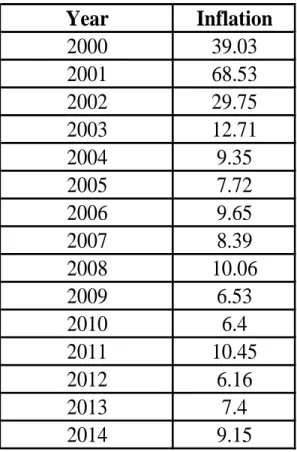
The schedule below shows the historic rate of inflation in turkey. The maximum rate of inflation was 68.5% in 2008 and the minimum rate of inflation was 6.4% in 2009.
Table 1. Turkey’s Yearly Inflation
Source:Turkstat
Year
Inflation
2000
39.03
2001
68.53
2002
29.75
2003
12.71
2004
9.35
2005
7.72
2006
9.65
2007
8.39
2008
10.06
2009
6.53
2010
6.4
2011
10.45
2012
6.16
2013
7.4
2014
9.15
13
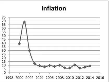
Figure 1. Turkey’s Inflation Source: Turkstat
2.1 The Consumer Price Index (CPI)
CPI is calculated and announced each month by the Bureau of Labor Statistics (BLS), is surely the most closely watched price index. When you read in the newspaper or see on television that the “cost of living rose by 0.2% last month,” may be the reporter is referring to the CPI.
To know which items is to be include and in what amounts, the BLS conducts an broad survey of spending habits more or less once every decade. As a consequence, the same bundle of merchandise and services is used as a standard for ten years or more (Baume, Blinder 2009).
Consumer price index is the main tool for measuring the inflation and price level in any country economy .It determine cost of living for a specific time.
Consumer price index can be calculated by the following formula.
0 5 10 15 20 25 30 35 40 45 50 55 60 65 70 75 1998 2000 2002 2004 2006 2008 2010 2012 2014 2016
Inflation
14
2.2 Inflation rate through CPI
When we speak about Turkey rate of inflation this is typically refers that the rate of inflation is apply on the consumer price index for a period. The CPI express the modification in cost of a regular bundle of merchandise and services that Turkish families buy for consumption .So as to measure rate of inflation an evaluation is prepared that what proportion of the CPI has go up in rate , over a given period contrast to the CPI in a previous period.
The annual rate of inflation is usually measured by CPI values.
15
3. Unemployment
The rate of unemployment shows that what is going on in the labor market. Unemployment goes down when the rate of those people who are out of work but are looking for work, over the entire people in the labor force falls. If in the society less people who are seeking work then employer shall trying to employee those who have already job.
Measurement of unemployment
Unemployment is measured by Bureau Labor Force Statistic by survey household .They ask people according to the following categories.
1) Employed: Those people who worked at least one hour for pay in last two week. These people may be those whose age is more than sixteen and they are working.
2) Unemployed: Those people who have now job and have not worked at one hour in last two weeks but the searched or spent for job at least one hour in last two weeks.
3) Not in labor force: People who have no job. These people may be those who are retired like grandfathers in the age of seventy years or a little kid whose age is less than 10 years. Those people whose age is more than sixteen and not seeking for job.
The labor force: All those people who are available for work it means Employed plus Unemployed people.
Adult civilian non institutionalized population
These are people who could potently be in a labor force, they are adult so they are legal to work, they are civilian so they are not in military, and they are non-institutionalized means they are not in jail or mental house facility. So these are all the people who available for work.
16
There are different types of unemployment first type is called Frictional Unemployment, in this kind of unemployment generally people are more capable for specific work and by their own will people quite their job and look for a better one. Second one is called Structural Unemployment, when the collective demand or collective supply structure is changing in any country than people may undergo through structural because of professional or geographic immobility. Third one is called Seasonal Unemployment; it takes place in a specific season where economic activities are concentrated during a few time periods. Fourth one is called cyclical unemployment, it occurs due to economic recession in which wages decreased.
The unemployment rate in Turkey
The unemployment rate is 9.7% which is 0.5 points higher than last year; 2.75 million people were unemployed According to TUIK‟s “Household Labor Force Statistics 2013”. The unemployment rate for non-agricultural was 12% in 2013. This rate was raised by 0.4% points to 11.5% in urban areas. Also it increased by 0.6 point to 6.1% in rural areas.
In the Southeast Anatolia region the highest rate of unemployment was recorded by 14.5% at the same time minimum rate of unemployment was recorded in Northeast Anatolia Region and in the West Black Sea Region with 6.7%. In addition there were fewer jobs for males with highest unemployment rate by 15.2% in Southeast Anatolia Region, and 14.8% unemployment rate were
17
The rate of employment rose from 45.4% to 45.9% from last year. 50% people were employed in services, 23.6% in agriculture, 19.4% in industry and 7% in construction. Employment in agricultural sector fell by 82 thousand people and nonagricultural go up by 785 thousand people as compared to 2012.
The unemployment rate among the age group 15 to 24 was 17.5 percent in the year 2012 and
now raise it to 18.7 percent in the year 2013.
Relating to the previous year the labor force participation rate was increased by 0.8 %points in 2013.But the labor force participation of male was 71.5% increased by 0.5 points, and 30.8% for female with an increase of 1.3 % points consider to previous year. The amount of out of the labor force decreased in 2013 from 27.4 million in 2012 to 27.3 million.
18
4. Time Series Analysis and Forecasting
Time series data are collected on a specific attribute by a phase of instance at ordinary periods. Techniques to forecasting the time series effort in account for changes by time through different methods. (Ken Black, 2009)
The analysis of time series consists in breaking down the observed series into various components parts for separate study. To achieve this breakdown we must have to make assumption about the relationship existing among the various components.
Time series is a set of data depending on time. There are lots of data which depends on time after some interval it changes. So we have to record our data and then on this basis we to the analysis.
An orderly arrangement of the statistical data by successive time period is called a time series. It is any set of data in which observation are arranged in a chronological order.
Examples of time series:
• The hourly temperature recorded in a city. • The daily consumption of electricity in a factory. • The weekly prices of sugar.
• The monthly sales of motor cycles. • The annual rainfall recorded in a city. • Total passengers carried by rail in a month. • Student enrollment in any university in a year.
19
4.1 Time series forecasting
According to (M.Shahzad 2011) a time series is a set of mathematical data that is obtained at equal intervals over time and forecasting is a process of assessing the magnitude of time series variable for some future point of time. Time series models can often be used more easily to forecast. Selecting an appropriate time series method is to be considering the type of data patterns. Four types of data patterns can be distinguished: stationary, seasonal, and cyclical and trend.
4.2 Forecasting
The desire to be able to foretell the future is a common characteristic of every human being. Business is an indispensable part of human activity .The common objective for every business man is to maximize the profit and to minimize the probable loss. The past has gone, the present is dealing with and the future we want to make safe and prosperous, which can be done by effective future planning based on past and present experience, thus it is future which worries human most and nobody can predict the future exactly but the past and present experiences always lead him to make certain predictions about the future. Forecasting in by the information we have at one time to guess what will happen at some future moment of time. (M.Shahzad2011)
The art or science of predicting the future which is utilized in the result and decision creation procedure to assist business community arrives at conclusions about trade, promotion, producing, hiring, and many other actions. For an example, think about the following items:
Market watchers predict a resurgence of stock values next year. City planners forecast a water crisis in Southern California. Future brightens for solar power.
20 Energy secretary sees rising demand for oil.
CEO says difficult times won‟t be ending soon for U.S. airline industry. Life insurance outlook fades.
Increased competition from overseas businesses will result in significant layoffs in the U.S. computer chip industry.
The aim of forecasting is to establish as accurately as possible, the probable behavior of economic activity based on all data available and to set policies in terms of these probabilities.
The forecast of future values are obtained through the data collected on past behavior of the variable to be predicated and on the behavior of other variable , forecasting is a scientific process which aims at reducing the uncertainty of the future state of business and trade.
4.2.1 Forecasting Methods
There are two types of forecasting methods quantitative and qualitative.
4.2.1.1 Quantitative forecasting
The method provide us accurate short term forecasting and can be used when the past data is available and it can be assumed that the patterns of past will continue into the near future i.e., present past is a good guide to the near future. (M.Shahzad 2011)
In such cases, a forecast can be developed either by time series method or a causal method .The qualitative approaches do not work well when sudden and major economic or political changes occur.
21
4.2.1.2 Qualitative forecasting
These methods can usually involves the use of intuitive thinking, specialist finding and accumulated knowledge to build up forecasts .These methods can be useful while the data on the variable being forecast can‟t be quantified and the past data are either not appropriate or unavailable (M.Shahzad 2011).
4.3 Components of a Time Series
Changes or variations in the observation of a time series are because of these four factors which are called component of the time series.
It is generally believed that data of time series are collected of four elements, trend, seasonal, cyclical, and irregular or random. (Ken Black, 2009)
4.3.1 The Trend Component (T)
The lengthy term common direction of data is referred to as trend. (Ken Black, 2009)
It is also called long term Secular trend with up and down movement of data more than five years. The common propensity of the data of time series to raise or decline in a lengthy period of time is called simply trend or secular trend. It is a flat normal and lengthy period progress of a time series. Its measurement helps in business planning. If we show the data on the graph than it is called linear line as Y=a +bx+e. Here the Least Squared Method is used to determine the trend.
4.3.2 The seasonal (S)
Also known as short time changes are those which are found daily , weekly , monthly or quarterly are caused mainly by the changing of seasons (weather or by holidays or by social
22
customs or by religious festivals).They are more or less regular movement within a 12 months period.
Example of seasonal variation are the production of soft drinks which is high during the summer and low during the winter, variations in daily temperature, the number of marriages on Friday and Sunday is higher than on any other day, near Eid the sales of clothes and shoes is increase considerably , etc.
4.3.3. Cyclical Component (C)
Cyclical variations are those rotational changes which occur according to the principle of business and economic in the form of cycles and are also called business cycles.
4.3.4 Irregular Component (I)
Irregular variations are unpredictable in nature and has no direction and amplitude as the other components of time series. The variations are caused by some unusual events. They are the result of enforceable causes such as floods, wars, strikes, elections famine etc are some examples of irregular variations. These variations being unseen cannot be controlled, so it‟s difficult to make a study of such non recurring variation.
23
4.4 Exponential Smoothing Methods
The exponential smoothing methods involve exponentially declining weights as the observation gets older. Exponential smoothing is one type of weighted average that assigns positive weights to past and current values. A single weight (α or ω) is called the exponential smoothing constant, is selected so it is between 0 and 1.
Thus an exponential series:
There for the exponential smoothing value at time “t” assigns the weight “ω” to the current series value and the weight (1-ω) to the pervious smoothed value. Like many average the exponential smoothing series changes less rapidly than the time series itself. The smoothness of depends on choice of “ω”. The smaller is the value of ω, the smoother is . The smoothed series is not affected by rapid changes in current values as small values of ω give more weight to the past value of the time series. A smooth series provides a good picture of the general trend of the original series. A major use of the exponential smoothing is to forecast future value of a time series. The past and current values of the time series are used in exponential smoothing so it is easily adapted to forecasting. The exponential smoothed forecast for is simply the smoothed
value at time t.
24
Note that for example the forecast for time t is the smoothed value for time (t-1). The forecast for time (t+1) is equal to the forecast for time t (Ft), plus a correction for the error in the forecast for in the forecast for time . An exponentially smoothed forecast is called an adaptive forecast for example the forecast for time (t+1) is explicitly adapted for the error in the forecast for time t. An exponential smoothing model assume that the time series has little or no trend or seasonal component, thus the forecast value is used to forecast not only but also all future value of .
4.4.1 Simple Exponential Smoothing
Simple exponential smoothing model is suitable for those time series in which there is no seasonality or trend. This method is so much similar with the model of A.R.I.M.A with 0 order of autoregression, differencing one order, moving average of one order and zero constant (Orhunbilge, 1999).
4.4.2 Brown's Linear / DoubleExponentialSmoothing
This model is the correct model for those time series which have a liner trend and no seasonality. These methods parameters are trend and level, and assumed to be equal. That‟s why this model has a unique folder of Holt‟s model. This method is so much similar with an A.R.I.M.A model with 0 order of autoregression, differencing 2 orders, moving average of 2 orders, coefficient for the 2nd order of moving average which is equal to the square of ½ of the coefficient for the 1st order.
25
4.4.3 Holt’s liner trend
Holt‟s liner trend model is the correct model for those time series which have a liner trend and zero seasonality. These methods parameters are trend and level, which are not forced by each other‟s value. This model may take lengthy time to work out for large series but this model is more common than Brown‟s model. This method is so much similar with an A.R.I.M.A model with 0 order of autoregression, differencing two orders, moving average of two orders and zero constant.
4.4.4 Holt Winters' Smoothing
C.C. Holt in 1957 firstly introduced this method by forthepurpose of nonseasonal time series which shows no trends. Holt laterly in 1958 made procedure which handle trends .After that Winters in 1965 mention a method to include seasonality , give the name “HoltWintersMethod”.
This method ha threee quations .Multiplicativ , additiveand with no trend. Each constant has ranges 0 to 1.
Multiplicative : Xt = (A+ Bt)* St +et
A and B are previously calculated initial estimates.St is the average seasonal factor for tth season.
This model is suitable for those time series in which have a linear trend and a seasonal effect, which does not depend in the level of the series. These methods parameters are trend, level, and season. There is no similarity in this method and ARIMA model.
Additive : Xt = (A+ Bt)+SNt + et
This model is suitable for those time series in which have a linear trend and a seasonal effect, which does not depend in the level of the series. These methods parameters are trend, level, and season. This method is so much similar with an ARIMA model with 0 order of autoregression, differencing one order, seasonal differencing one order, moving average of P+1 orders, as of P is the seasonal interval of the number of periods.
26 No Trend :β= 0, so, Xt = A * SNt +et
Ġt means exponential smoothing is similar to the Holt winters smoothing if and .
4.5 Autoregressive Model
A forecasting technique that takes benefit of the relationship of values (Yt) to the previous period values is called autoregression. (Ken Black, 2009)
Autoregression is a numerous regression method with in which the self determining factor or independent variables are time lagged volume of the needy variable; it means we forecast a value of from values of . The independent variable can be lagged for 1, 2, 3, or more time periods. An autoregressive model containing independent variables for three time periods looks like this: (Ken Black, 2009).
Autoregression is helpful tool in finding seasonal or cyclical effects in the data of time series. For example, if any data are given in 12 months increments, autoregression using lagged variables by 12 months can search for the predictability of previous monthly time periods. If data are given in quarterly time periods, autoregression of up to four periods removed can be a useful tool in locating the predictability of data from previous quarters. When the time periods are in years, lagging the data by yearly periods and using autoregression can help in locating cyclical predictability (Ken Black, 2009).
In autoregressive forecasting, the dependent variable (y) is treated the same way it is in other regression models within this chapter. However, each independent variable represents previous values of the dependent variable (Ronald, J. Brian, Lawrence, 2008).
27
4.5.1 First order autoregressive model
The forecast for specific time is calculated by the value experimental by the previous time period (Ronald, J. Brian, Lawrence, 2008).
̂
Where
4.5.2 Second order autoregressive model
The forecast for specific time is calculated by the value experimental by the 2 previous time period (Ronald, J. Brian, Lawrence, 2008)
̂ Where
4.5.3 Data Source
Mostly mentioned data is secondary data taken from the following research website for the period 2000 to 2014.
1. Turkish Statistical Institute www.turkstat.gov.tr 2. Central Bank of Turkey-TCMB www.tcmb.gov.tr
28
4.5.4 Practical work through Autoregressive Model
These steps are taken place for building Autoregressive Model
1. Create an excel sheet , Where we have to put time series data than run analysis by doing regression analysis, the highest-order parameter within the autoregressive model to be evaluated, realizing that the t test for significance is predicated on degrees of freedom. 2. Create a table for different lagged variable for Lag1, Lag 2, Lag3, and Lag4. The 1st p
lagged forecast variable lags by only one phase , the 2nd p lagged forecast variable lags by two time phase, then on and therefore the last forecaster variable lags by p time periods.
3. Complete a least-squares analysis containing all p lagged forecaster variables of the multiple regression model using excel.
4. Check takes a look at for the significance or importance of the highest order autoregressive parameter within the model.
If null hypothesis is not rejected then remove pth variables and do again step three and four by doing that the test of significant of the new highest order parameter shall be based on T distribution whose degrees of freedom are revised to correspond with revised range of forecasters.
If the null hypothesis is rejected, choose the autoregressive model with all p predictors for fitting to forecasting.
29 Table 2. Turkey’s Inflation with Lags
Year Inflation Lag 1 Lag 2 Lag 3 Lag 4
2000 39.03 2001 68.53 39.03 2002 29.75 68.53 39.03 2003 12.71 29.75 68.53 39.03 2004 9.35 12.71 29.75 68.53 39.03 2005 7.72 9.35 12.71 29.75 68.53 2006 9.65 7.72 9.35 12.71 29.75 2007 8.39 9.65 7.72 9.35 12.71 2008 10.06 8.39 9.65 7.72 9.35 2009 6.53 10.06 8.39 9.65 7.72 2010 6.4 6.53 10.06 8.39 9.65 2011 10.45 6.4 6.53 10.06 8.39 2012 6.16 10.45 6.4 6.53 10.06 2013 7.4 6.16 10.45 6.4 6.53 2014 9.15 7.4 6.16 10.45 6.4 Source: Turkstat
30 Table 3. Excel Output of Lag 4
For selecting a proper and best fitted autoregressive model for the annual time series I shall start with the fourth order autoregressive model.
̂
Next step is to test for the significance of the highest order parameter. The highest order parameter estimate, for the fitted fourth order autoregressive model is -0.025854, with a standard error of 0.038589.
SUMMARY OUTPUT
Regression Statistics
Multiple R
0.549425839
R Square
0.301868753
Adjusted R Square -0.16355208
Standard Error
1.665660969
Observations
11
ANOVA
df
SS
MS
F
Significance F
Regression
4
7.197895757 1.799473939 0.64859313
0.648402082
Residual
6
16.64655879 2.774426465
Total
10
23.84445455
Coefficients Standard Error
t Stat
P-value
Lower 95%
Upper 95% Lower 95.0% Upper 95.0%
Intercept
13.00156906
3.498672237 3.716143778 0.00989739
4.44062652 21.5625116 4.44062652 21.56251161
Lag 1
-0.45743206
0.360463861 -1.26900949 0.25144179 -1.339455353 0.42459123 -1.33945535 0.424591232
Lag 2
-0.28256051
0.303642228 -0.93057052 0.38798493
-1.02554627 0.46042526 -1.02554627 0.460425258
Lag 3
0.167678145
0.129185334 1.29796579 0.24195926 -0.148426981 0.48378327 -0.14842698 0.48378327
31 Testing null hypothesis:
T-Test value= -0.6699859
Using α=0.05 level of significant the two tail test t test with 6 degrees of freedom has critical value ±2.447.Because -2.447˂-0.6699 and +2.447˃-0.6699 or because the p value= 0.5277954˃0.05 I cannot reject therefore it can be concluded that the fourth order parameter of the autoregressive model is not significant and can be deleted.
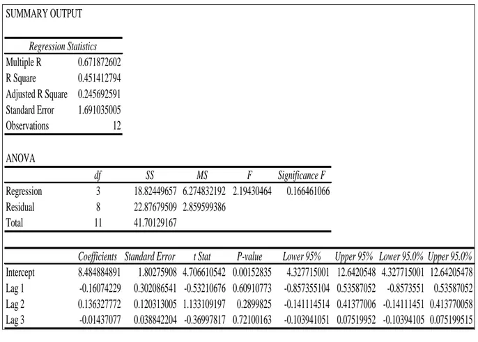
Table 4. Excel Output of Lag 3
3rd autoregressive model ̂ SUMMARY OUTPUT Regression Statistics Multiple R 0.671872602 R Square 0.451412794 Adjusted R Square 0.245692591 Standard Error 1.691035005 Observations 12 ANOVA df SS MS F Significance F Regression 3 18.82449657 6.274832192 2.19430464 0.166461066 Residual 8 22.87679509 2.859599386 Total 11 41.70129167
Coefficients Standard Error t Stat P-value Lower 95% Upper 95% Lower 95.0% Upper 95.0% Intercept 8.484884891 1.80275908 4.706610542 0.00152835 4.327715001 12.6420548 4.327715001 12.64205478 Lag 1 -0.16074229 0.302086541 -0.53210676 0.60910773 -0.857355104 0.53587052 -0.8573551 0.53587052 Lag 2 0.136327772 0.120313005 1.133109197 0.2899825 -0.141114514 0.41377006 -0.14111451 0.413770058 Lag 3 -0.01437077 0.038842204 -0.36997817 0.72100163 -0.103941051 0.07519952 -0.10394105 0.075199515
32
Next step is to test for the significance of the highest order parameter. The highest order parameter estimate, for the fitted 3rdorder autoregressive model is -0.01437, with a standard error of 0.038842204.
Testing null hypothesis:
T -Test value= -0.3699782
Using α=0.05 level of significant the two tail test t test with 8 degrees of freedom has critical ±2.306.Because -2.306˂-0.369978 and +2.306˃-0.369978 or because the p value= 0.72100˃0.05 I cannot reject therefore it can be concluded that the third order parameter of the autoregressive model is not significant and can be deleted.
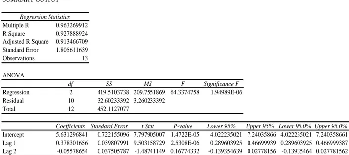
Table 5. Excel Output of Lag 2
2nd autoregressive model ̂ SUMMARY OUTPUT Regression Statistics Multiple R 0.963269912 R Square 0.927888924 Adjusted R Square 0.913466709 Standard Error 1.805611639 Observations 13 ANOVA df SS MS F Significance F Regression 2 419.5103738 209.7551869 64.3374758 1.94989E-06 Residual 10 32.60233392 3.260233392 Total 12 452.1127077
Coefficients Standard Error t Stat P-value Lower 95% Upper 95% Lower 95.0% Upper 95.0%
Intercept 5.631296841 0.722155096 7.797905007 1.4722E-05 4.022235021 7.24035866 4.022235021 7.240358661 Lag 1 0.378301656 0.039807991 9.503158729 2.5308E-06 0.289603925 0.46699939 0.289603925 0.466999387 Lag 2 -0.05578654 0.037505787 -1.48741149 0.16774332 -0.139354639 0.02778156 -0.13935464 0.027781562
33
Next step is to test for the significance of the highest order parameter. The highest order parameter estimate, for the fitted 2nd order autoregressive model is -0.055786, with a standard error of 0.037505787.
To test the null hypothesis:
T- Test value= -1.4874115
Using α=0.05 level of significant the two tail test t test with 10 degrees of freedom has critical ±2.288.Because -2.288˂-0.369978 and +2.288˃-0.369978 or because the p value= 0.16774˃0.05 I cannot reject therefore it can be concluded that the 2nd order parameter of the autoregressive model is not significant and can be deleted.
34 Table 6. Excel Output of Lag 1
First order Autoregressive model
̂
Next step is to test for the significance of the highest order parameter. The highest-order parameter estimate, for the fitted 1st order autoregressive model is 0.612704, with a standard error of 0.204130656.
Testing the null hypothesis:
T test value= 3.0015329
Using α=0.05 level of significant the two tail test t test with 12 degrees of freedom has critical ±2.179.Because t statistic 3.00153˃2.179 or because the p value= 0.0110352˂0.05 I can reject
therefore it can be concluded that the first order parameter of the autoregressive model is significant and should remain in the model.
SUMMARY OUTPUT Regression Statistics Multiple R 0.654844754 R Square 0.428821652 Adjusted R Square 0.381223457 Standard Error 13.09411095 Observations 14 ANOVA df SS MS F Significance F Regression 1 1544.679024 1544.679024 9.00919975 0.011035214 Residual 12 2057.468898 171.4557415 Total 13 3602.147921
Coefficients Standard Error t Stat P-value Lower 95% Upper 95% Lower 95.0% Upper 95.0% Intercept 4.287343998 4.86852884 0.880624135 0.39581615 -6.320269087 14.8949571 -6.32026909 14.89495708 Lag 1 0.612704881 0.204130656 3.0015329 0.01103521 0.167942389 1.05746737 0.167942389 1.057467373
35
For the given data of inflation the most appropriate model is the first order autoregressive model. Using the estimates and and the most recent data or year value .
For forecasting year 2015 inflation the equation would be like that.
̂
̂
̂
̂
̂
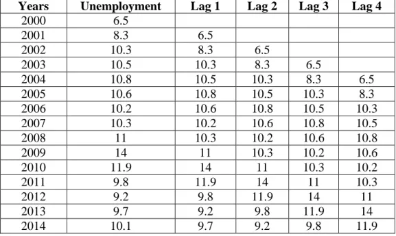
Table 7. Turkey’s Yearly Unemployment with Lags
Years Unemployment Lag 1 Lag 2 Lag 3 Lag 4
2000 6.5 2001 8.3 6.5 2002 10.3 8.3 6.5 2003 10.5 10.3 8.3 6.5 2004 10.8 10.5 10.3 8.3 6.5 2005 10.6 10.8 10.5 10.3 8.3 2006 10.2 10.6 10.8 10.5 10.3 2007 10.3 10.2 10.6 10.8 10.5 2008 11 10.3 10.2 10.6 10.8 2009 14 11 10.3 10.2 10.6 2010 11.9 14 11 10.3 10.2 2011 9.8 11.9 14 11 10.3 2012 9.2 9.8 11.9 14 11 2013 9.7 9.2 9.8 11.9 14 2014 10.1 9.7 9.2 9.8 11.9 Source: Turkstat
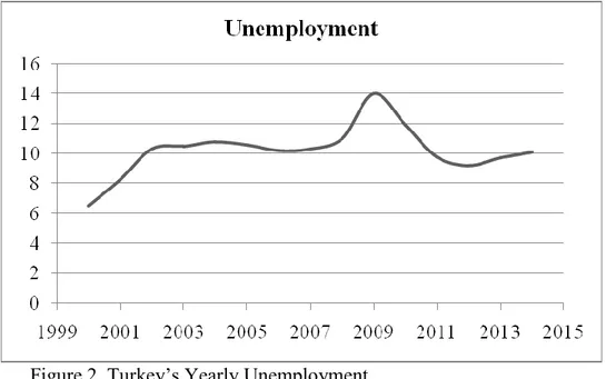
36
Figure 2. Turkey‟s Yearly Unemployment Source: Turkstat
Table 8. Excel Output of Lag 4 for Unemployment
SUMMARY OUTPUT Regression Statistics Multiple R 0.650798643 R Square 0.423538874 Adjusted R Square 0.039231456 Standard Error 1.288083822 Observations 11 ANOVA df SS MS F Significance F Regression 4 7.314131311 1.828532828 1.10208353 0.434964578 Residual 6 9.954959598 1.659159933 Total 10 17.26909091
Coefficients Standard Error t Stat P-value Lower 95% Upper 95% Lower 95.0% Upper 95.0%
Intercept 10.70791156 5.586357923 1.916796544 0.10372582 -2.961413821 24.3772369 -2.96141382 24.37723694 Lag 1 0.586139095 0.390354452 1.501556064 0.18389038 -0.369023839 1.54130203 -0.36902384 1.541302029 Lag 2 -0.45130055 0.456872856 -0.98780338 0.36139408 -1.569228154 0.66662705 -1.56922815 0.666627053 Lag 3 -0.138428023 0.459331667 -0.30136834 0.77330522 -1.26237212 0.98551607 -1.26237212 0.985516075 Lag 4 0.004071531 0.297112664 0.013703661 0.9895107 -0.722936966 0.73108003 -0.72293697 0.731080028
37
For selecting a proper and best fitted autoregressive model for the annual time series I shall start with the fourth order autoregressive model.
̂
Next step is to test for the significance of the highest order parameter. The highest order parameter estimate, for the fitted fourth order autoregressive model is 0.0040, with a standard error of 0.01370.
Testing null hypothesis:
T test value= 0.0137
Using α=0.05 level of significant the two tail test t test with 6 degrees of freedom has critical ±2.447.Because 2.447˃0.0137 or because the p value= 0.9895˃0.05, I cannot reject therefore it can be concluded that the fourth order parameter of the autoregressive model is not significant and can be deleted.
38 Table 9. Excel Output of Lag 3 for Unemployment
3rd autoregressive model
̂
Next step is to test for the significance of the highest-order parameter. The highest-order parameter estimate, for the fitted 3rd order autoregressive model is 0.0314, with a standard error of 0.27244.
Testing the null hypothesis:
T- Test value= 0.1154
Using α=0.05 level of significant the two tail test t test with 8 degrees of freedom has critical SUMMARY OUTPUT Regression Statistics Multiple R 0.593608992 R Square 0.352371635 Adjusted R Square 0.109510999 Standard Error 1.183511184 Observations 12 ANOVA df SS MS F Significance F Regression 3 6.09691022 2.032303407 1.45092115 0.298848415 Residual 8 11.20558978 1.400698723 Total 11 17.3025
Coefficients Standard Error t Stat P-value Lower 95% Upper 95% Lower 95.0% Upper 95.0% Intercept 8.006135529 3.917279185 2.043800085 0.0752288 -1.027126462 17.0393975 -1.02712646 17.03939752 Lag 1 0.637527251 0.354134023 1.800242872 0.10951235 -0.17910727 1.45416177 -0.17910727 1.454161773 Lag 2 -0.422975528 0.380673476 -1.11112424 0.29879033 -1.300810137 0.45485908 -1.30081014 0.454859081 Lag 3 0.031459113 0.272445522 0.11546937 0.91091886 -0.596801386 0.65971961 -0.59680139 0.659719612
39
±2.306.Because 2.306˃0.1154 or because the p value= 0.910˃0.05 I cannot reject therefore it can be concluded that the third order parameter of the autoregressive model is not significant and can be deleted.
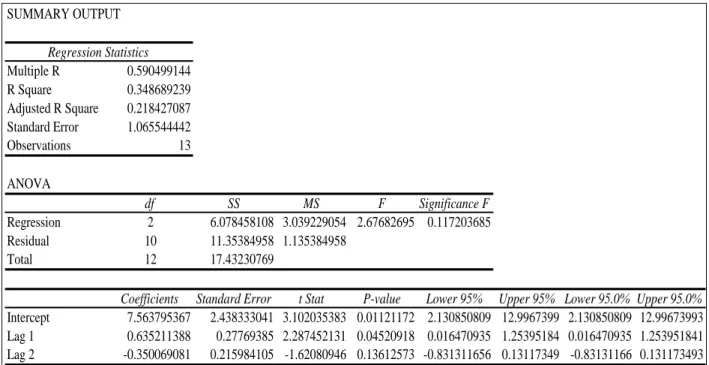
Table 10. Excel Output of Lag 2 for Unemployment
2nd autoregressive model
̂
Next step is to test for the significance of the highest order parameter. The highest-order parameter estimate, for the fitted 2nd order autoregressive model is -0.3500, with a standard error of 0.2159.
Testing the null hypothesis:
T- Test value= -1.6208 SUMMARY OUTPUT Regression Statistics Multiple R 0.590499144 R Square 0.348689239 Adjusted R Square 0.218427087 Standard Error 1.065544442 Observations 13 ANOVA df SS MS F Significance F Regression 2 6.078458108 3.039229054 2.67682695 0.117203685 Residual 10 11.35384958 1.135384958 Total 12 17.43230769
Coefficients Standard Error t Stat P-value Lower 95% Upper 95% Lower 95.0% Upper 95.0% Intercept 7.563795367 2.438333041 3.102035383 0.01121172 2.130850809 12.9967399 2.130850809 12.99673993 Lag 1 0.635211388 0.27769385 2.287452131 0.04520918 0.016470935 1.25395184 0.016470935 1.253951841 Lag 2 -0.350069081 0.215984105 -1.62080946 0.13612573 -0.831311656 0.13117349 -0.83131166 0.131173493
40
Using α=0.05 level of significant the two tail test t test with 10 degrees of freedom has critical value ±2.288.Because -2.288˂-1.6208 and +2.288˃-0.369978 or because the p value= 0.1361˃0.05 I cannot reject therefore it can be concluded that the 2nd order parameter of the autoregressive model is not significant and can be deleted.
Table 11. Excel Output of Lag 1 for Unemployment
First order Autoregressive model
̂
Next step is to test for the significance of the highest order parameter. The highest-order parameter estimate, for the fitted 1st order autoregressive model is 0.4572, with a standard error of 0.1814. SUMMARY OUTPUT Regression Statistics Multiple R 0.588168191 R Square 0.345941821 Adjusted R Square 0.291436973 Standard Error 1.10848272 Observations 14 ANOVA df SS MS F Significance F Regression 1 7.798764152 7.798764152 6.34699173 0.026942642 Residual 12 14.74480728 1.22873394 Total 13 22.54357143
Coefficients Standard Error t Stat P-value Lower 95% Upper 95% Lower 95.0% Upper 95.0%
Intercept 5.804995692 1.878598126 3.090067861 0.00936115 1.711881998 9.89810939 1.711881998 9.898109385 Lag 1 0.457233126 0.181490426 2.519323665 0.02694264 0.061799457 0.85266679 0.061799457 0.852666795
41 Testing the null hypothesis:
T-Test value= 2.519
Using α=0.05 level of significant the two tail test t test with 12 degrees of freedom has critical value ±2.179.Because t statistic 2.519˃2.179 or because the p value= 0.026˂0.05 I can reject therefore I conclude that the first order parameter of the autoregressive model is significant and should remain in the model.
For the given data of employment the most appropriate model is the first order autoregressive model.
Using the estimates and and the most recent data or year value
For forecasting year 2015 Unemployment the equation would be like that.
̂ ̂
̂
̂
42
4.5.5 Phillips curve
A lot of debate takes place among the economists that to discuss possibility to attain two macroeconomics goals at the same point for instance low unemployment and low inflation. About this the theory of Phillips curve emerged. This theory shows a tradeoff between unemployment and inflation. Discussion on the subject of the reality of negative relationship involving unemployment and inflation has take much significance when renowned economist Whilliam Phillips wrote a article about “The Relationship between Unemployment and the Rate of change of Money wage Rates in the united kingdom 1861-1957”. Later than the journal of Bill Phillips (1958) the central focus of policy maker and macroeconomists has been remained to find the relationship between unemployment and inflation. The main purpose of the debate was to confirm the relation between inflation and unemployment either there exist negative relation or not.
There are three important assumptions to understand the Phillips curve firstly In short run the tradeoff can be seen between unemployment and inflation. Secondly the tradeoff can be break by stagflation in the short. Thirdly in the long run there is no exchange or tradeoff between inflation and unemployment. It is true that increase in the prices of daily use goods set dreadful outcome on the consumer purchasing power. Now consumers are enforced to buy the same commodities at a costly rate. Unexpected increases in price enforce consumers to buy less as they can‟t take the load. Because of this consumers are paying extra income to get a smaller amount of goods at high prices. When prices are goes up by the time ability of consumers to purchase goods goes down, by that a raise in unemployment take place in the economy.
The short run Phillips curve has a negative slope, its means as the inflation has increasing so the unemployment will decrease. When you have the high price level means more output when there is more output it means more people are working. So higher output means lower unemployment and by this worker will have more leverage, more options. Employers shall raise wages to attract and retained workers then workers will have more power to buy goods and services which will increase demand. When demand increase for goods and services is going to increase the all utilization of factors of production (Land, Labor, Capital, Organization or Entrepreneurship).
43
Assumption of Short Run Phillips Curve are That two variables must remains constant 1) expected rate inflation 2) natural unemployment rate means cyclical unemployment is zero.
In short run economy faces a tradeoff between inflation and unemployment. When monetary and fiscal policy maker expand aggregate demand and movie the economy up along the Short Run Aggregate Supply Curve they can low unemployment for a sometime but only at the cost of high inflation rate.
When monetary and fiscal policy maker contract aggregate demand and movie the economy down along the Short Run Aggregate Supply Curve they can lower inflation rate but only at the cost of temporally higher unemployment.
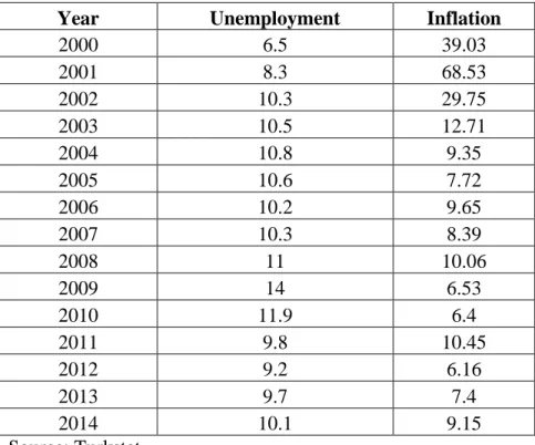
4.5.6 Relationship between unemployment and inflation
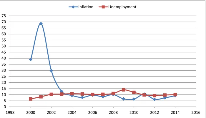
Table 12. Turkey’s Yearly Unemployment and Inflation
Year Unemployment Inflation
2000 6.5 39.03 2001 8.3 68.53 2002 10.3 29.75 2003 10.5 12.71 2004 10.8 9.35 2005 10.6 7.72 2006 10.2 9.65 2007 10.3 8.39 2008 11 10.06 2009 14 6.53 2010 11.9 6.4 2011 9.8 10.45 2012 9.2 6.16 2013 9.7 7.4 2014 10.1 9.15 Source: Turkstat
44
Figure 3. Combined Unemployment and Inflation Source: Turkstat
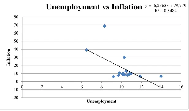
4.5.7 Simple Linear Regression Model
In accordance with all empirical studies, it is suggested that the equation for Inflation (I) is expressed as a function of Unemployment (UN). That can be expresses in the following equations.
I = α + β1 (UN)
Whereas in equation I represent the dependent variable i.e. Inflation, independent variables is Unemployment (UN). 0 5 10 15 20 25 30 35 40 45 50 55 60 65 70 75 1998 2000 2002 2004 2006 2008 2010 2012 2014 2016 Inflation Unemployment