Investigations on the effects of fourwave-mixing in dwdm fiber channels

T.C. DOĞUŞ UNIVERSITY

GRADUATE SCHOOL OF SCIENCE ENGINEERING AND TECHNOLOGY DEPARTMENT OF ELECTRONICS AND COMMUNICATIONS

ENGINNEERING

INVESTIGATIONS ON THE EFFECTS OF FOURWAVE-MIXING IN DWDM FIBER CHANNELS

M.Sc. THESIS

Onur ERKAN

Thesis Advisor: Prof.Dr. Ercan TOPUZ

ii

T.C. DOĞUŞ ÜNİVERSİTESİ

ELEKTRONİK VE HABERLEŞME MÜHENDİSLİĞİ BÖLÜMÜ

INVESTIGATIONS ON THE EFFECTS OF FOURWAVE-MIXING IN DWDM FIBER CHANNELS

M.Sc. THESIS

Onur ERKAN 200892001

Thesis Advisor: Prof.Dr. Ercan TOPUZ

iii FOREWORD

I would like to thank the all people who supported me carrying out this work, without their help and support this thesis would not have been possible.

Firstly, I like to extend my gratitude to my academic supervisor Prof. Dr. Ercan Topuz for accepting me as Ms candidate. Especially I want to thank for his encouragements and guidance throughout the thesis. His deep insights and expertises in fiber optics have made this work possible.

I want to thank my wife Feyza Erkan for her support and patience during thesis with an everlasting positive energy and motivation. I would also like to thank my parents for their unconditional support during the time I studied.

Finally I would like to express my gratitude to Technology Division of Vodafone Turkey for the opportunity to write my thesis on such a related topic with industrial focus area of fiber optics communications.

iv TABLE OF CONTENTS FOREWORD iii TABLE OF CONTENTS iv ABSTRACT v ÖZET vii LIST OF FIGURES ix LIST OF TABLES x 1. INTRODUCTION 1

1.1 Background and Problem Definition 2

1.2 Introduction to Optical Fibers in Communication Systems 3

1.3 WDM Optical Fiber Communication Systems 4

1.4 Overview and Objective of the Thesis 6

2. THEORY OF OPTICAL FIBERS 8

2.1 Fiber Types 9

2.2 Linear Degradation 10 2.2.1. Attenuation in Fibers 10

2.2.2. Chromatic Dispersion 12

2.2.3. Polarization Mode Dispersion 13

2.3 Nonlinear Degradation 14

2.3.1. Self Phase Modulation 15

2.3.2. Cross Phase Modulation 16

2.4 Four Wave Mixing 17

2.4.1. Introduction 18

2.4.2. Interchannel and Intrachannel Effects 19

2.4.3. FWM Efficiency 20

2.4.4. FWM Effect Reduction Techniques 21

3. PULSE PROPAGATION IN WDM OPTICAL FIBER COMMUNICATION SYSTEMS 22

3.1 Wave Propagation Equation 23

3.2 Fiber Modes 24

3.2.1. Single Mode Condition 25

3.3 Derivation of pulse propagation equation 27 4. NUMERICAL ALGORITHM AND SIMULATIONS 33 4.1 Numerical method to solve NLSE 34 4.2 Symmetrized Split step fourier method 35 4.3 Simulations 38 4.4 Results 38 REFERENCES 67 APPENDIX 75

v

INVESTIGATIONS ON THE EFFECTS OF FOURWAVE-MIXING IN DWDM FIBER CHANNELS

ABSTRACT

Optical fiber cables have become ideal for achieving the challenge of reaching high speed data rates and terabit transmission, due to its low attenuation characteristics and high bandwidth capability such as 50 THz. Multiplexing of numerous channels on the same fibre requires higher transmit power or sufficiently lower fibre losses to utilize the available bandwidth having high bit rate with a span of thousands of kilometer.

It is required to increase the number of optical channels in dense WDM systems in order to meet the extreme capacity demands on data transmission networks. This necessity of increment in number of channels can be provided only with small channel spacing. In order to reach required amount of signal channels, new frequency standards such as 25 GHz and 12.5 GHz were recently specified by ITU. In such narrower channel spacing with large number of WDM channels, the non-linear effects of the optical fibre can induce serious system impairments. In modern WDM systems, the primary nonlinear effects are cross phase modulation (XPM), and the four-wave mixing (FWM). The FWM characteristics are especially related to frequency allocation of channels. Throughout this thesis, we will be mainly dealing with the FWM impairments.

The occurrence of FWM depends on several factors, such as frequency spacing between channels, the input power per channel, the dispersion characteristics of the optical fiber, and the distance along which the channels interact.

Four wave mixing results from changes in the refractive index with optical power called optical Kerr effect. In FWM, two co-propagating waves produce two new optical sideband waves at different frequencies. The generation of these beat signals which fall into original signal wavelengths causes a channel energy loss, which induces a crosstalk effect. In long haul transmission links, the deployment of optical amplifiers makes the problem even worse, as not only the transmitted signal is amplified, but also the generated FWM products, which mix again with the signals, causing new products. Also when intense incident signal power launched into a fiber, linearity of optical response is lost. Moreover, in the usage of dispersion-shifted fibers (DSF), the FWM mechanism is enhanced, due to a depletion of the phase mismatch associated to the fiber's chromatic dispersion. In consequence, the detected signal power will fluctuate considerably.

Numerous techniques have been proposed to minimize the detrimental limiting effects of FWM such as: the spectral allocation of the channels, the spectral assignment of the channels as far as possible from the zero-dispersion wavelength (λZD), and the spectral distribution of the unequally spaced channels, which requires a complex system design. In this study, the impact of the channel spacing (positioning of the DWDM channels), phase mismatching, changing of channel input power and fiber length on FWM efficiency were analyzed based on represented algorithm. For various types of fibers such as G.652

vi

(Single- Mode Fiber - SMF), G.653 (Dispersion-Shifted Fiber - DSF), and G.655 (Non-Zero Dispersion-Shifted Fiber - NZDSF) compliant fibers, considering the DWDM grids suggested by the ITU-T Recommendations G.692, and G.694.1, with uniform channel spacing of 100, 50, 25, and 12.5 GHz were compared with simulations. Split Step Fourier Method (SSFM) numerical technique has been used to model nonlinear Schrödinger (NLS) equation in order to investigate pulse propagation in optical fibers.

vii

DALGA BOYU BÖLMELİ ÇOĞULLAMA SİISTEMLERİNİN FİBER KANALLARINDA DÖRT DALGA-KARIŞIMI ETKİLERİNİN İNCELENMESİ

ÖZET

Fiber optik kablolar, düşük zayıflama özellikleri ve 50 THz gibi yüksek bant genişliği sağlayabilen profilleri sayesinde yüksek hızlı verilerin aktarımına ulaşmak için ideal hale gelmiştir. Aynı fiber üzerinden, binlerce kilometrelik mesafelerde yüksek bit hızı ile mevcut bant genişliği kullanmak için çok sayıda kanalın çoğullanması, yüksek iletim gücü yada kaybı yeterince düşük fiber gerektirir.

Veri iletimi şebekelerinde artan kapasite taleplerini karşılamak amacıyla yoğun dalga boyu bölmeli çoğullama (WDM) sistemlerinde optik kanal sayısını artırmak gerekmiştir. Gerekli olan bu kanal sayısı artışı sadece kanal aralığı küçük tutularak sağlanabilir. İstenen sayıda sinyal kanalına ulaşabilmek için uluslar arası telekomünikasyon kurumu (ITU) tarafindan belirlenen son frekans aralıkları olan 25 GHz ve 12.5 GHz frekanslar kullanılmaktadır. Bu denli yakın kanal boşlukları kullanılarak elde edilen WDM sinyalleri, optik fiberin doğrusal olmayan etkileri sebebiyle ciddi sistem bozukluklarına neden olabilir. Modern WDM sistemlerinde doğrusal olmayan etkilerin başlıcaları Çapraz-Faz Modülasyonu (XPM) ve Dört-Dalga Karışımı (FWM), sistem performansını sınırlandırmaktadır. FWM etkisinin karakteristiği özellikle kanalların frekans düzlemindeki tahsisi ile ilişkilidir. Bu tez boyunca, FWM bozuklukları ve etkileri ele alınıp incelenmiştir.

FWM oluşumu; kanallar arası frekans aralığı, kanal başına giriş gücü, optik fiberin dispersiyon özellikleri ve kanalların aldığı mesafe boyunca birbirleri ile etkileşimi gibi birçok faktöre bağlıdır.

Dört dalga karışımı, “Optik Kerr Etkisi” adı verilen fiber kırılma indisinin optik güç ile değişiminden gelmektedir. FWM etkisinde, eş yayılan iki dalga farklı frekanslarda iki yeni optik yan dalga üretmektedir. Bu bozucu yan dalga ürünlerinin orijinal sinyal kanalları üzerinde oluşması sonucu enerji kaybı meydana gelmekte ve çapraz karışım etkisine sebep olmaktadır. Uzun mesafeli veri iletim hatlarında, optik kuvvetlendiricilerin kullanılması; problemi daha da ciddileştirmekte olup iletilecek ana sinyal ile beraber FWM ürünü sinyallerin de kuvvetlendirilmesine, karışıma sebep olacak yeni ürünler doğmasına sebep olmaktadır. Ayrıca fibere yoğun bir giriş sinyali uygulandığında optik doğrusallık bozulmaktadır. Buna ilaveten Dispersiyonu Kaydırılmış Fiber (DSF) kullanılması durumunda, fiberin kromatik dispersiyonu ile ilişkili olarak faz uyumsuzluğunun azalması sonucu FWM etkisi gelişir. Bunun sonucu olarak elde edilen edilen sinyal gücü önemli ölçüde dalgalanır.

FWM ve sınırlayıcı etkilerinin minimize edilmesi için sayısız teknik geliştirilmiştir. Kanalların spektral dağılımı, sıfır-dispersiyon dalga boyundan (λZD) mümkün olan en uzak

viii

mesafede kanalların seçimi ve eşit olmayan bir spektral dağılım, karmaşık bir sistem tasarımı gerektiren tekniklerdir.

Bu tez çalışmasında, kanal aralığının etkisi (DWDM kanal konumlandırması), faz uyuşmazlığı, kanal giriş gücünün ve fiber uzunluğunun değişiminin FWM verimliliği üzerinde etkisi sunulan algoritma kullanılarak analiz edilmiştir. ITU-T G.692 ve G.694.1 DWDM kanal dağılım standardları olan 100, 50, 25 ve 12.5 GHz kanal aralıkları ile fiber standartları olan G.652 basamak-indisli tek modlu optik fiber (step-index, SMF), G.653 dispersiyonu kaydırılmış fiber (DSF) ve G.655 sıfırlanmamış dispersiyonu kaydırılmış fiber (NZDSF) türleri simülasyonlarda karşılaştırılmıştır. Simülasyonlarda optik fiberin darbe yayılımını sayısal teknik ile araştırmak amacıyla parçalı adım Fourier metodu (SSFM) ile doğrusal olmayan Schrödinger (NLS) denklemi çözülmektedir.

ix LIST OF FIGURES

Page

Figure 1.1: Cross section and refractive-index profile for step-index and

graded-index fibers ... 3

Figure 1.2: Schematic view of a DWDM System ... 5

Figure 2.1: Standard geometrical parameters and index profiles for optical fibers (a) graded-index MMF, (b) step-index SMF ... 7

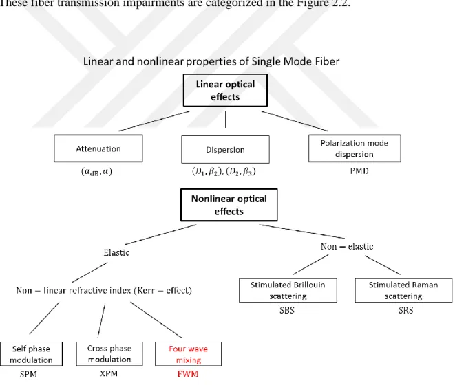
Figure 2.2: Linear and non-linear optical fiber effects ... 8

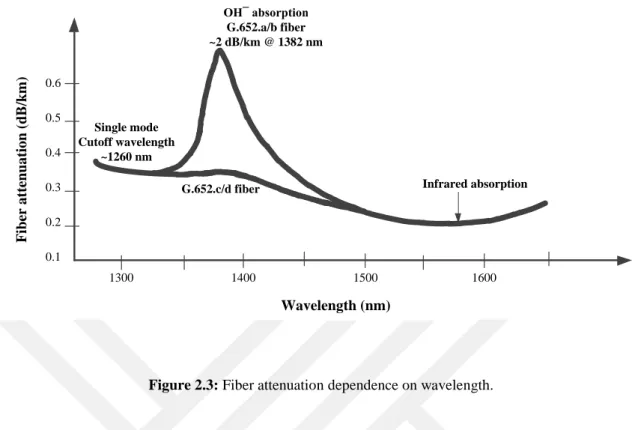
Figure 2.3: Fiber attenuation dependence on wavelength ... 10

Figure 2.4: Pulse spreading due to chromatic dispersion in fiber ... 11

Figure 2.5: Total chromatic dispersion in SMF resulting from material and waveguide dispersion ... 14

Figure 2.6: Differantial group delay (PMD) effect on pulse propagation ... 16

Figure 2.7: FWM products of three equally spaced DWDM signals ... 20

Figure 2.8: Number of FWM products ... 21

Figure 2.9: FWM efficiency for different channel spacing with respect to different values of chromatic dispersion ... 23

Figure 2.10: Cross sectional area of a G.655 fiber ... 24

Figure 3.1: Normalized propagation constant b as a function of normalized frequency V for a few low-order fiber modes. ... 31

Figure 4.1: Schematic view of SSFM process ... 38

Figure 4.2: FWM power change along with the fiber length with respect to different dispersion parameters. ... 41

Figure 4.3: Variation of FWM Efficiency with different channel spacing for different dispersion parameters. ... 42

Figure 4.4: Variation of FWM Power with different channel spacing for different types of fiber. ... 43

Figure 4.5: FWM Noise Power change with Injected power ... 44

Figure 4.6: FWM Noise Power change with Injected power ... 44

Figure 4.7: Produced FWM components for equidistant 3 channel DWDM system ... 45

Figure 4.8: Graphical user interface ... 46

Figure D.1: Focus of Gaussian beam ... 55

Figure D.2: Normalized Gaussian beam Intensity as a function of t ... 46

Figure F.1: Flow diagram of the symmetric Split-Step Fourier Method for solving the Nonlinear-Schrödinger Equation ... 61

x LIST OF TABLES

Page

Table 2.1 : FWM products of three equally spaced DWDM channels. ... 4

Table 4.1: Characteristics of different types of optical fibers. ... 4

Table H.1: Transmission data rates for SONET/SDH ... 65

1 1. INTRODUCTION

1.1 Background and Problem Definition

The rapid increase of worldwide communication, internet and multimedia demands has led to an explosive growth of high speed digital communications. Throughout the latter quarter of the 20th century fiber optics has been indispensable in facilitating this extraordinary load [1].

Modern commercial fiber optic systems are capable of transmitting hundreds of gigabits-per-second, with experimental systems demonstrating terabit capability [2]. Contemporary optical fibers have a bandwidth in excess of 30 terahertz [3]. While the fiber channel may be capable of transmitting terabit-per-second (Tb/s) data rates, no current single electrical communication system can reach this capacity. The electrical transmitters and receivers on either end of a fiber channel are subject to technological constraints currently which limit their speeds at about 40 Gb/s [4].

Communication systems overcame the electronic limitations with the invention of low-loss optical fibers and wavelength division multiplexing (WDM) thereby resulting in an increment in the transmission capacities [3].

In WDM systems, the available bandwidth is divided into separate channels with each channel carrying one signal. The data rate of each channel frequently limited to 10 Gb/s, but total data rate of all channels are much higher [2]. In order to increase the transmission capacity of WDM optical system, transmission data rate per wavelength has been increased as well as the number of wavelengths.

However, there are two different transmission issues which are limiting factors in long-haul WDM systems: dispersion and fiber nonlinearities.

In terms of the high data rate transmission, the chromatic dispersion (CD) and polarization-mode dispersion (PMD) are typically major obstacles which result in much larger penalties than the nonlinearity of optical fiber. Thus, nonlinear effects were usually neglected prior to the 1990’s. With the improvement of dispersion shifted fibers (DSF), dispersion compensating fibers (DCF) and the other dispersion management techniques, the limiting problem of CD has been mitigated [5,6].

2

As data rates have continued to increase the number of wavelengths the number of wavelengths also increased. Decreasing channel spacing in WDM systems led to limitations due to nonlinearities such as four-wave mixing (FWM) and cross-phase modulation (XPM).

In order to establish communications over long-haul networks the power losses are compansated by using erbium-doped single mode fiber amplifier (EDFA) at about every 50 km in WDM transmission systems.

Although EDFAs make the high optical power levels available in WDM systems, they also led to a more vulnerable system performance by increasing nonlinear effects [7,8]. This leads to interference, distortion, and excess attenuation of the transmitted signals and results in system degradations. As a result, fiber nonlinearities emerged as the most serious limiting factor.

The origin of nonlinearities arise from the variation of the refractive index in an optical fiber that is related to the intensity of the optical signal. This detrimental effect becomes more significant when high aggregate power is launched, even if the individual power of each channel may be below the level needed to produce nonlinearities. The combination of high total optical power and large number of channels at narrower spaced wavelengths leads to the formation of many unwanted components. Hence, four-wave mixing seems to be the most harmful impairment in dense wavelength division multiplexing (DWDM) systems [9-11].

1.2 Introduction to Optical Fibers in Communication Systems

An optical fiber is a dielectric waveguide consisting a core region which has a higher refractive index surrounded by a cladding layer that has lower refractive index material. This type of fiber is called step-index fiber. This refractive index difference ensures that the propagating signal power is contained predominantly within the core region which has a higher refractive index. For propagation, the angle of incidence of the propagating light should be smaller than the critical angle at the boundary waveguide. For core region with a refractive index n , and for the cladding region with a refractive index _c n , the critical _cl

3 arcsin cl c c n n   _ _   (1.1)

Another parameter used to characterize an optical fiber is Numerical Aperture (N.A.). Numerical aperture is the maximum angle that light can be accumulated into a fiber from its end faces and can be calculated with Snell-law:

 

sin _{c cl}

NA   n n (1.2)

where refractive index of environment is taken as “1” considering incidence from air. As opposed to step-index fibers, the graded-index fibers have a refractive index profile which has its highest value on the axis and decreases monotonically towards the index of the cladding region. Figure 1.1 shows schematically the index profile and the cross section for the two kinds of fibers.

a b

a b

Step-index fiber Graded-index fiber

Jacket Cladding Core b a n1 n2 n0 In d ex Radial distance b a n1 n2 n0 In d ex Radial distance

Figure 1.1: Cross section and refractive-index profile for step-index and graded-index fibers [2].

The normalized frequency which is denoted as V determines the number of modes supported by an optical fiber and can be expressed as

1

2 2 2

0 ( c cl)

4

where k₀ 2_ ,  is the core radius, and  is the wavelength of the light. It is observed that the V parameter depends on the geometry of fiber and the core-cladding index difference. Industrial fibers are designed to support only one mode that can be satisfied by the V<2.405 condition. A step-index fiber which satisfies this condition is referred as Single-mode fiber(SMF). In this thesis, only single mode fibers are investigated with different classification of ITU such as G.652, G.653, G.655 fibers. Fiber modes will be explained in more detail in the following chapter.

1.3 WDM Optical Fiber Communication Systems

A standard communication system consists of basic components like multiplexer, demultiplexer, signal source, receiver and carrier medium. In order to use the system in full capacity, a new technique is developed through the simultaneous multiplexing of each channel. Time division multiplexing (TDM) and Frequency division multiplexing (FDM) are two main multiplexing schemes which use time domain and frequency domain respectively. In practice, these two multiplexing techniques can be used both in electrical domain and optical domain. Due to the limitations imposed by electronic components, transmission of multiple channels over same fiber provided a simple way for exploiting the large bandwidth offered by optical fibers. Development of such system corresponds to optical carriers at different wavelengths, which is called Wavelength Division Multiplexing (WDM) [2].

Wavelength division multiplexing (WDM) is a technology used to combine and split two or more optical signals of different optical center wavelengths in a fiber. This technique allows fiber capacity to be expanded in the frequency domain from one channel to more than 100 channels.

The WDM channel wavelength assignment is an industry standard defined in International Tele-communications Union (ITU-T) recommendation (See Appendix-G).

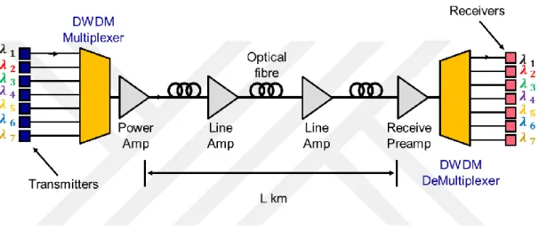
In a typical WDM system (Figure 1.2), bit sequence is modulated in transmitters through optical carriers each at a different wavelength i.e., λ1 … λN with a specific modulation format. Optical bandpass filtering and combining of the individual wavelength signals are performed in multiplexer level. The demultiplexer coupler separates the combined signals

5

through their corresponding channel ports. Basic WDMs are transparent to all optical protocols such as SONET, SDH, GigE, 10GigE, etc. They are also transparent to transmission rates up to the WDM’s specification limits (Appendix-H).

During signal propagation several linear and nonlinear fibre impairments such as attenuation, chromatic dispersion and fibre nonlinearities affect the system. The main focus of this thesis is to study the effects of four-wave mixing (FWM) which is considered as a major limitation in a Dense Wavelength Division Multiplexing System [12].

Figure 1.2: Schematic view of a DWDM System.

When low loss SMF is used (e.g, fibers with reduced OH-absorption near 1.4µm), the ultimate capacity of a WDM system can reach up to 300 nm bandwidth. The minimum channel spacing can be as small as 50 GHz or 0.4 nm for 40-Gb/s channels. Since 750 channels can fit into the 300-nm bandwidth, the resulting effective total bit rate may be as large as 30 Tb/s. Assuming that the WDM signal can be transmitted over 1000 km by using optical amplifiers with dispersion management, the effective BL product may exceed 30,000 (Tb/s).km with the usage of WDM technology [2].

1.4 Overview and Objective of the Thesis

This thesis is focused on the several degradation effects of four-wave mixing in high capacity DWDM systems. The propagation algorithm is used to calculate linear and nonlinear fiber transmission parts. The long-haul scenario is unique in the sense that it

6

simultaneously requires high data rates, high power levels and long distances. This is precisely the condition under which nonlinear effects are the limiting factor.

The thesis is organized as follows. The problem definition and some preliminaries on optical communication channels are given in Chapter 1.

Chapter 2 introduces the theoretical background of pulse propagation equation in fiber optic transmission systems. Linear and nonlinear fibre impairments effecting the transmission are presented. All of the high capacity WDM systems transmit multiple-channels on a single fiber with high spectral efficiency. The performance in these systems is limited by the inter-channel non-linearities (XPM, FWM) due to the interaction of neighbouring channels. The main focus of this work will be the effect of FWM as the most problematic nonlinear impairment of DWDM systems. The impact of intra-channel and inter-channel nonlinear effects of FWM is analyzed at 10 and 40 Gbit/s.

The signal propagation in a fiber channel can be described by the nonlinear Schrodinger

equation (NLSE) and the solution of the NLSE can be solved numerically by using split-step Fourier method (SSFM).

In Chapter 3 numerical solution of pulse propagation equation is presented. Software simulations performed in Matlab with Split Step Algorithm (SSFM). Optisystem, (or Linksim) a commercial software is used to compare and verify results. SSFM algorithm is implemented by solving the linear and nonlinear part in an iterative method numerically. All the simulation results derived are given in Chapter 4. The conclusions are summarized. Several future research directions are also suggested and discussed in this chapter.

7 2. THEORY OF OPTICAL FIBERS 2.1 Fiber Types

An introduction to the theory of optical fibers was given in Section 1.2. In terms of the ray optics, approximation for propagation is described by the Snell’s law and Total Internal Reflection. The fibers with higher fractional index change Δ are not suitable for optical communications due to the multipath dispersion (modal dispersion). For this reason, another type of fiber is developed with considerably reduced intermodal dispersion. Such an optical fiber is called as graded-index fiber (GRIN) [2].

Graded-index fibers have a core with radially decreasing refractive index from the center to the core boundary. Considering the geometrical properties and the number of guided modes, the fibers can be categorized further as multi-mode and single mode fibers.

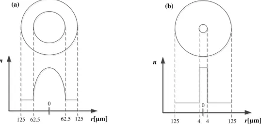
The graded index profile is usually given as:





where  is the core radius. The parameter  determines the index profile. n is the ₁

nominal refractive index n₁n r ( 0), n is the refractive index of the homogeneous ₂

cladding, ρ is the radius of the core, 2 2 2

1 2 1

(n n ) 2n

   . A step-index profile is approached in the limit of large . A parabolic-index fiber corresponds to  2.

n r[µm] (a) 0 125 62.5 n r[µm] (b) 0 125 4 62.5 125 _{4 125}

Figure 2.1: Standard geometrical parameters and index profiles for optical fibers

8

For optical communication systems, optical fibers are assumed to be a perfect data transmission medium considering bandwidth limitations of the other mediums. Several limitations are taken into account especially in high bit rate systems, as the distance and number of amplifiers increase. These limitations can be divided into two major categories: linear and nonlinear.

The linear propagation effects of the fibers are attenuation, chromatic dispersion (CD) and polarization mode dispersion (PMD).

In particular, the nonlinear effects set strict limitations for multiwavelength WDM systems at higher bit rates and increased distances. The primary nonlinear effects are self phase modulation (SPM), cross phase modulation (CPM) and four-wave mixing (FWM).

These fiber transmission impairments are categorized in the Figure 2.2.

9 2.2 Linear Degredation

2.2.1. Attenuation in Fibers

Average optical power P of a bit stream propagating inside an optical fiber differs and it can be shown by Beer’s formula:

dP

P

dz   (2.2)

where  is the attenuation coefficient.

Optical power loss is wavelength dependent and cumulative in an optical fiber. It increases exponentially with fiber length,

( )

0

( , ) z j t z

x

E z t E e e   W (2.3)

The amount that an optical signal is attenuated in power after propagating through a passive component or fiber can be defined as optical loss and given by

exp( )

out in

P P L (2.4)

where P is the transmitted power, _out P is the initial power and _in 𝐿 is the length of the fiber. The value of  can be expressed in units of dB/km using the relation

10 10 ( ) log out 4.343 in p dB km L p    _ _    (2.5)

Elastic collisions between the light wave and fiber molecules cause the scattering of light along the entire length of the fiber. This type of scattering is also known as Rayleigh scattering. Some of the light escaping from the fiber waveguide and some of the light reflecting back to the source is a direct outcome of Rayleigh scattering that causes 96% of (attenuation) signal loss in fibers. However, the other factors such as material absorption and bending loss account for the rest.

10 0.1 0.2 0.3 0.4 0.5 0.6 1300 1400 1500 1600 Single mode Cutoff wavelength ~1260 nm OH¯ absorption G.652.a/b fiber ~2 dB/km @ 1382 nm Infrared absorption G.652.c/d fiber Wavelength (nm) F ib er a tt en u a ti o n ( d B /k m )

Figure 2.3: Fiber attenuation dependence on wavelength.

Absorption of light energy by fiber impurities such as water (OH−) molecules is called material absorption. The main water absorption band is centered at 1383 nm, which is considerably reduced in newer G.652.c/d fiber. Figure 2.3 shows fiber attenuation dependence on wavelength of a typical standard G.652.a/b fiber and reduced water absorption G.652.c/d fiber.

2.2.2. Chromatic Dispersion

Variation in propagation delay with respect to wavelength results in broadening of the pulses. This phenomenon is referred as Chromatic Dispersion (C.D.) which depends on fiber materials and dimensions.

Phase velocity of a propagating wave (carrier velocity) is related to propagation parameter β as defined in the equation below

eff c n      (2.6) eff

n is the effective refractive (mode) index that is related to propagation constant: 0

eff

n k

11

where k is the wave number and defined as ₀ k₀  c2 .

For a single mode fiber (SMF), the major source of dispersion is the group velocity dispersion (GVD). Group velocity (pulse envelope velocity or information velocity) is defined as derivative of the phase velocity,

1 1 ( ) 1 g d d  _    _  (2.8)

where  is the propagation constant.

The wavelength dependence of the group velocity leads to pulse broadening due to the dispersion of different spectral components during propagation. Resulted time delay (Fig. 2.4) can be determined as g T L v (2.9) λ1 λ2 λ3 λ4 λ5 v1 v2 v3 v4 v5 Tb Input pulse {λ1...λ7} group Fiber core Longest wavelength Δτ Relative group delay Shortest

wavelength Tb +Δτ

z

Output pulse spread

Figure 2.4: Pulse spreading due to chromatic dispersion in fiber [12].

Using Equation 2.9, the extent of broadening (T) for a pulse spectral width of Δω through a fiber of length L is governed by

2 2 2 g dT d L d T L L d d v d                _ _       (2.10) 2

 is known as the group velocity dispersion (GVD) parameter. It’s used to present pulse broadening parameter of the optical signal while propagating inside the fiber.

Dispersion coefficient can also be derived from the propagation constant with expansion of Taylor-series as

12 0 ₀ 2 2 0 2 0 1 ( ) ( ) ( ) 2 d d n c d   d                          (2.11) where 2 2 2 d d   

 is group velocity dispersion (GVD) (2.12)

Spectral width of the optical pulse is defined as





2 c

   

    (2.13)

Substituting Equation 2.13 in Equation 2.10, broadening of pulse can be written as

g d L T DL d v       _ _     (2.14) where 1 2_{2 2} g d c D d v     _  _ _    (2.15)

D is called dispersion coefficient and can be expressed by the group velocity dispersion, β2,

2 2 2 c D      ps/(km-nm) (2.16)

dispersion slope is also often expressed in terms of wavelength using the dispersion slope parameter 2 3 2 0 0 2 2 dD c S D d  _       _{ }    (2.17)

where the slope parameter S is normally given in ps/nm2/km. A typical value in SMF at 1550 nm is 0.08 ps/nm2/km.

Material dispersion and waveguide dispersion are the two subproducts of total dispersion in optical fibers.

Predominant one material (intermodal) dispersion appears in MMF because the different modes are associated with different velocities. Material dispersion occurs due to the fiber core’s refractive index changing with wavelength.

13 1 g M dn D c d  (2.18)

where n_g is the group index defined as n_g n_eff  (dn_eff d).

At the wavelength of 1.276 µm, slope of n_g becomes zero (dn_g d0). This wavelength is referred to as zero-dispersion wavelength_ZD. For the region below _ZD,D is negative _M

and above that it becomes positive. Zero dispersion wavelength of the fibers can vary depending on doping the core and cladding which results in with a refractive index variation based upon design.

The main cause of the waveguide dispersion effect is the physical structure of the fiber core cladding that causes pulses to propagate at different velocities for different wavelengths.

Waveguide dispersion depends on fiber design parameters such as core radius  and core-cladding index difference ∆. It can be calculated as

2 2 2 2 2 2 g ( ) g ( ) W n Vd Vb dn d Vb D n dV d dV                 (2.19)

Since the result of this equation is always negative, D is negative throughout the entire _W

wavelength range [2].

If the total dispersion is considered (Figure 2.5) as the combination of material and waveguide dispersion, it reduces to

M W

DD D (2.20)

As the pulse propagate in fiber, signal pulse becomes wider due to chromatic disperison which leads to two major problems:

1) Trailing and leading edges of the pulse spreads into adjacent pulse bit time slots which is called as Inter Symbol Interference (ISI),

14 Zero dispersion wavelength Material dispersion Total chromatic dispersion Wavelength dispersion Wavelength D is p er si o n c o ef f. ( p s/ (n m .k m )) + -0 - - - - -1200 _{1300 λ}ZD 1400 1500 1600 nm

Figure 2.5: Total chromatic dispersion in SMF resulting from material and waveguide dispersion [4].

Typical values of dispersion are in the range 15–18 ps/(km-nm) near 1.55µm. In WDM communication systems, this wavelength region has remarkable interest.

Using this feature, new fibers designed such that whose zero dispersion wavelength are shifted towards the longer wavelengths.

Most commonly deployed fiber type is Standard Single Mode Fiber (SMF, ITU-T G.652) which has a non-dispersion shifted structure. Therefore it is also known as Non-Dispersion Shifted Fiber (NDSF). Zero dispersion wavelength of SMF is approximately 1310 nm. They are used for both TDM and DWDM transmission systems with the dispersion compensation requirement.

Dispersion-shifted fibers (DSF, ITU-T G.653) have its zero dispersion wavelength in 1550 nm region. This property reduces dispersion for this window whereas increasing nonlinear distortions especially FWM in deployment for DWDM links.

The other type of fiber has a low chromatic dispersion window in 1550 nm region but not zero. Those fibers which are designed to alleviate nonlinear distortions is known as Non-zero Dispersion Shifted Fiber (NZDSF, ITU-T G.655). Because of the reasons, these fibers are frequently preferred in multichannel DWDM systems.

Also fibers with the positive ₂ value ,(D negative) in the wavelength region below 1.6 µm are designated to compensate dispersion in communication links. This type of fiber is called dispersion compensating (DCF) fiber [12].

15 2.2.3 Polarization Mode Dispersion

Ideally, single mode fibers have perfectly cylindrical and circular core. But in industry the core of the fibers exhibit variations in the shape along with the fiber length due to mechanical and thermal stresses included during manufacturing and deployment. The change of geomety results in a difference between index of refraction and the orthogonally polarized modes.

This phenomenon is referrred to as birefrigence and defined as m x eff y eff

B  n _ n _ (2.21)

where n_{x eff} and n_{y eff} are mode indices for orthogonally polarized modes.

A periodical power exchange between these two orthogonal polarization components occurs because of the birefrigence. This period is called beat length and can be calculated as B m L B   (2.22) Typically L_B 10 m at 1µm.

As a result of birefrigence, initially launched linear polarization quickly reaches a state of arbitrary polarization.

These two principal states of polarization have different velocities that lead to pulse spreading along the fiber. The amount of pulse spreading in time between the two polarization pulses is referred to as differential group delay (DGD) and is measured in units of picoseconds (Figure 2.6).

Differential group delay is given by

1x 1y ( 1) gx gy L L T L L v v           (2.23)

When both of the polarization components of input pulse excited into a waveguide fiber, pulse becomes broader as the components disperse due to different propagation velocities (also for different frequency components) of the signal’s two orthogonal polarizations.

16

This phenomenon is called polarization-mode dispersion (PMD) and turns out to be a restrictive factor for optical communication systems operating at high bit rates.

Input intensity Fiber core Instantaneous DGD z Output Intensity seen by receiver X Y Slow PSP vx vy Fast PSP Input vx=vy vx vy Differential group Delay (DGD) nx > ny vx < vy Due to DGD

Figure 2.6: Differential group delay (PMD) effect on pulse propagation [3].

It can be calculated as;

p T D ps km L   (2.24)

where T is the differential group delay and L is the length of the fiber as a transmission distance.

PMD value is in the range of 0.1-1 ps/√km. Because of its √L dependence, PMD induced pulse broadening is relatively small as compared to GVD effects [2,12].

2.3 Nonlinear Degredations

The refractive index of the fiber is assumed to be constant at low power levels. This assumption makes silica as a linear medium. In other words the fiber material (silica) is assumed to be linear medium.

Even though silica is intrinsically not a highly nonlinear material, the waveguide geometry confines light to the small core cross section and hence power density becomes several hundreds of MW/m2 . Thus, over long fiber spans nonlinear effects become significant in the design of WDM communication systems.

Effect of nonlinear impairments is dependent on signal strength which declines exponentially along with the propagation in the fiber. Therefore, effective fiber length is defined as the length of fiber beyond which nonlinear effects are no longer significant.

17 0 ( ) L eff in P z dz L P 



where P is the initial optical power, L is the fiber length and _in P z is the power of the ( ) optical signal at length of z. P z is related to the attenuation in the fiber: ( )

( ) _in z

P z P e (2.26)

Thus L_eff can be reduced to

1 L eff e L      (2.27)

Typically α is 0.048/km (αdB = 0.21 dB/km) at 1550 nm, then Leff is approximately 21 km for very long (where L>> 21 km) nonamplified fiber links.

Nonlinear effects in optical fiber mainly originate from fiber’s refractive index dependence on intensity of the propagating signal which is referred to as Kerr effect. Variation in refractive index due to the Kerr effect is caused by two reasons.

First one is the change in refractive index due to the high signal power levels. This change in refractive index can be calculated as

2 ( , ) _eff( ) eff p n E n n A     (2.28)

where A_eff is the effective fiver core area, n is the nonlinear index coefficient. Typical ₂

values of n are 3.0 x 10₂ -20 _m2_{/W (varies between 2.0 x 10}-20 _{to 3.5 x 10}-20 _m2_{/W) for silica.} Second significant reason of nonlinear Kerr effect is the change in refractive index due to the change of propagation parameter (β) by a factor called nonlinear coefficient (). It can be derived by

' P

    (2.29)

where ' is the nonlinear propagation parameter.

In practice nonlinear coefficient () varies between 1 to 3 (1/km.W) And it can be obtained by

18 2 2 eff n A     (2.30) 2.3.1 Self-phase modulation

Nonlinear coefficient term (  ) produces a pahse shift which increases linearly along with the propagation distance z. This nonlinear phase modulation induces a pulse on itself which referred as Self-Phase Modulation (SPM). Assuming the constant input power, nonlinear phase shift due to SPM is given by

0 0 ( ) ( ) L L SPM in eff ' dz P z dz P L  





where P z and ( ) L_effare defined in Equation (2.26) and (2.27) respectively.

SPM leads to frequency chirping of optical pulses which depends on the pulse shape. In order to reduce the impact of SPM, phase shift value _SPM should be less than 0.1. For long fibers, this assumption can be approximated to

0.1 ( )

in A

P   N (2.32)

In practice, if =2 (1/W.km), NA=10, α=0.2 dB/km, the input peak power is limited to 2.2 mW.

2.3.1 Cross-phase modulation

The nonlinear behaviour of the refractive index due to the optical intensity of other channels creates phase shift (i.e. frequency modulation) for a specific channel. This phenomena is known as cross-phase modulation (CPM or XPM) which occurs especially in multichannel transmission systems such as DWDM.

Phase shift of the j-th channel can be written as

( 2 ) XPM j eff j m m j L P P     



Assuming equal channel powers worst case of the phase shift occurs when pulses completely overlap one another. In this case phase shift can be estimated as

19

( ) (2 1)

XPM

j M Pj

     (2.34)

Pulses at different wavelengths travel at different group velocities in the presence of dispersion and cause walk-off between pulses. This process diminishes the distortions induced by XPM. Therefore, the effect of XPM is inversely proportional to dispersion discrepancies among channels in WDM systems [2,12].

2.4 Four-Wave Mixing

2.4.1 Introduction

In WDM transmission, when three optical signals of different center wavelengths are propagating through an optical fiber, beating (mixing) of the signals leads to generation of interfering signals at new wavelengths. This process is called as Four-Wave Mixing (FWM). This newly produced signal is called FWM component which can cause signal crosstalk if the frequency falls within the band of an existing WDM channel. FWM originates from the dependence of the fiber’s refractive index on the intensity of optical signal that produces a nonlinear medium due to the third order nonlinear susceptibility. If the number of channels are increased, number of FWM light is also increased. It can be expressed as

4 1 2 3

     (2.35)

But only frequency combinations of ₄   ₁ ₂ ₃ are generate significantly high power components in WDM systems provided that the channel spacing and dispersion are small enough to meet the phase matching condition.

FWM process is also different from SPM and XPM because of energy transfer between channels. Such a power transfer not only results in the power loss for the channel but also induces interchannel crosstalk that degrades the system performance seriously.

20 C37 C36 C35 C34 C33 C32 C31 C30 DWDM Channels P o w er DWDM Signals Newly generated FWM products λ113 _λ112 λ213 λ123 λ223 λ132 λ312 λ221 λ332 λ321 λ231 λ331 λ1 _{λ2 λ}3

Figure 2.7: FWM products of three equally spaced DWDM signals [12].

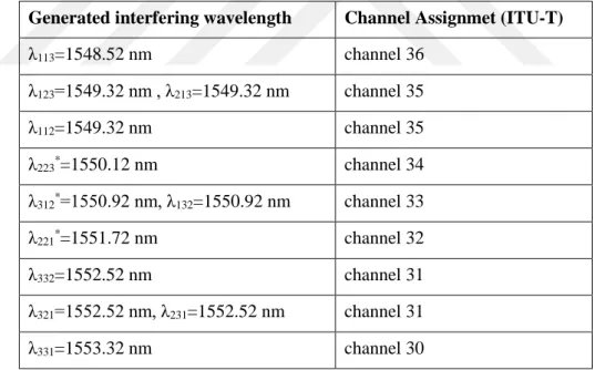
In Table 2.1 three equally spaced DWDM channels (λ1=1550.12, λ2=1550.92, λ3=1551.72 nm) and FWM components is presented. Generated FWM terms are given in Table 2.1.

Table 2.1: FWM products of three equally spaced DWDM channels.

Generated interfering wavelength Channel Assignmet (ITU-T)

λ113=1548.52 nm channel 36 λ123=1549.32 nm , λ213=1549.32 nm channel 35 λ112=1549.32 nm channel 35 λ223*=1550.12 nm channel 34 λ312*=1550.92 nm, λ132=1550.92 nm channel 33 λ221*=1551.72 nm channel 32 λ332=1552.52 nm channel 31 λ321=1552.52 nm, λ231=1552.52 nm channel 31 λ331=1553.32 nm channel 30

The generated components with center wavelengths λ223=1550.12, λ312=1550.92, λ221=1551.72 fall directly into the original DWDM signal channels therefore causing interference. The other generated components fall into adjacent and nearby DWDM channels interfering with those channels (Figure 2.7) [2,12].

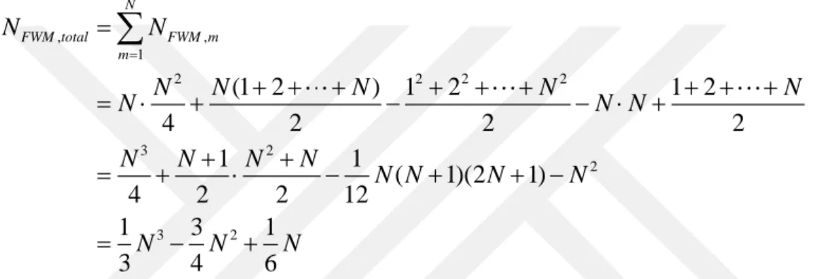
21 2 ( 1) 2 N N (2.36) where N is the number of DWDM channels.

Assuming channels are equally spaced and number of channels are even, the number of these FWM components on the m-th signal channel is expressed as

2 2

4 2 2 2

FWM

N Nm m m

N     N (2.37)

Therefore, the total number of the FWM components that fall on the signal channels can be calculated as: , , 1 2 2 2 2 3 2 2 3 2 (1 2 ) 1 2 1 2 4 2 2 2 1 1 ( 1)(2 1) 4 2 2 12 1 3 1 3 4 6 N FWM total FWM m m N N N N N N N N N N N N N N N N N N N N N                              



As number of channels increases, generated FWM products increases rapidly.

22 2.4.2 FWM Efficiency

FWM leads to crosstalk and this resulting with the generation of new wave at frequency can be defined by

FWM i j k

    

Types of mixing are divided to two categories as degenerate and non-degenerate. Degenerate involves FWM components that do not appear on the original DWDM signal channels (f_i  f_j  f_k). Nondegenerate involves FWM components that can appear on the same original DWDM signal channels (f_i  f_j  f_k) .

Assuming all signals have the same polarization along the propagation in the fiber and no amplifiers are used, the power of FWM component can be calculated as

2 2 2 1 ( ) 9 L ijk i j k eff P   d PP P L e (2.39)

where  is the efficiency and d is the degeneracy factor which defined as

3, 6, ijk i j d i j     _ 

FWM efficiency can be obtained as

2 2 2 2 2 4 sin ( 2) 1 (1 ) L L e L e              _  _   _  _ (2.40)

where  is the phase mismatch.

Assuming same channel spacing, phase mismatch parameter can be given by (Appendix-E). 2 2 fc 2 CD ( ) 2 k k ik jk c ik jk f f f f S c c          _     _   (2.41)

Assuming the same channel spacing, depending on the distance of center wavelength of the DWDM system to the zero-dispersion wavelength phase mismatch parameter , ,can be reduced to

23 4 2 0 0 0 2 2 2 0 2 ( ) is near 2 is far from i m m c m f f f S c D f c  _{ }   _{ }         _  (2.42)

The FWM efficiency is shown in Figure 2.9 as a function of channel spacing. Fiber dispersion coefficient for a 100 km fiber span with attenuation is also taken 0.21 dB/km at 1550 nm. As the fiber’s dispersion coefficient or channel spacing increases, the FWM efficiency decreases, thereby reducing the power of FWM component. As the CD increases, the FWM becomes negligible especially for the broader channel spacing.

Channel spacing Δf (GHz) F W M e ff ic ie n cy η ( d B ) 40 20 60 80 100 120 140 160 180 200 -50 -40 -30 -20 -10 CD=8 ps/(nm.km) CD=17 ps/(nm.km) CD=1 ps/(nm.km)

Figure 2.9: FWM efficiency for different channel spacing with respect to different values of chromatic

dispersion [12].

For the long-distance transmission in WDM system, if the standard SMF is employed at 1550nm window, a cumulative CD will degrade the system performance. Due to the GVD, different channels travel at different speeds thereby lowering FWM efficiency.

When the perfect phase matching occurs the efficiency takes its the highest value, e.g. in a fibre without chromatic dispersion. Higher fibre dispersion and larger channel spacing decrease the phase matching [13].

24 2.4.3 Reducing FWM Effect

Numerous techniques have been proposed to reduce the effect of FWM-induced degradation on WDM systems. Generally these techniques focused on the minimizing of FWM terms that intersect with WDM channels. These techniques consist of

1- Designing WDM systems with unequal channel spacing: In order to prevent overlapping of generated FWM components on the WDM channels, uneven channel spacing can be designed.

2- Designing WDM systems with wide channel spacing: As the spacing between DWDM channels are increased, phase-matching is decreased with a result of reduced FWM efficiency.

3- Reducing transmitter signal power and amplifier spacing can help diminishing the FWM effect.

4- Deploying a fiber with larger cross sectional area (i.e. ITU-T G.655). Larger effective area reduces the optical intensity and consequently effects of FWM.

Large Effective Area NZDSF Aeff=72µm2 NZDSF Aeff=55 µm2 Radius (µm) Light Intensity Effective Area

Figure 2.10: Cross sectional area of a G.655 fiber.

5- Using polarization-multiplexed DWDM channels can reduce FWM component power and cross talk.

25

If deployed optical fiber is not a ITU G.655 type fiber, another practical and applicable solution is to plan a dispersion-management map such that GVD is high locally all along the fiber even though its average value is quite low. Such a dispersion map can be realized with the combinations of fibers with normal and anomalous GVD. Consequently, locally high GVD leads to reduce of phase mismatch and hence resulting in a reduced FWM crosstalk [13].

26

3. PULSE PROPAGATION IN WDM OPTICAL FIBER CHANNEL 3.1 Wave Propagation Equation

Maxwell equations govern the propagation of optical fields. , t      D H J (3.1) , t      B Ε (3.2) . _f,  D (3.3) . 0,  B (3.4)

where E and H are electric and magnetic field vectors, D and B are corresponding electric and magnetic flux densities, J and ρf are current density vector and the charge density, respectively.

Since following assumptions can be made:  There are no free charges _f = 0.

 Conductivity is very close to zero ( 0, assuming a lossless medium J. , E J0).  Silica is a nonmagnetic material.

The flux densities D and B are related to the electric and magnetic fields E and P propagating inside the medium as

0    D Ε P (3.5) 0   B H (3.6)

where ε0 = 8.885 × 10-12 As/Vm is the vacuum permittivity, μ0 = 1.2566 ×10-6 Vs/Am is the vacuum permeability, and P is the induced electric polarization.

Equations 3.1 to 3.4 take the following form for propagation in optical fibers

B t      Ε (3.7) D t     H (3.8) . 0 D (3.9) . 0  B (3.10)

27

Putting equations (3.1), (3.2), (3.5) and (3.6) together and taking the curl leads to

( ), t       Ε B (3.11) 0 ( 0 ) , t  t          _{ }  _     Ε Ε P (3.12) 2 2 0 0 2 0 2 t t            Ε P Ε (3.13) where 0 0 2 1 , c    (3.14) Equation (3.13) yields 2 2 0 2 2 2 1 c t  t         Ε P Ε (3.15)

In order to solve Equation (3.15), a relation between induced polarization vector P and electric field vector E is needed.

Induced polarization consists of two parts: linear (PL) and nonlinear (PNL) . ( , )t  _L( , )t  _NL( , ).t P r P r P r (3.16) (1) 0 ( , ) ( ). ( , ) , L t   t t' t' dt'   



_{  }

Since optical fibers (silica) are isotropic and symmetric compounds, second order nonlinear susceptibility is ignored in calculations.

Nonlinear part of polarization is a result of third order susceptibility χ(3) as explained in (Appendix-A)

Due to the weakness of nonlinear effecs in silica fibers; it’s considered as PNL has a small perturbation on total polarization. It will be assumed as PNL = 0 and only linear part of the polarization will be taken into account as a first step.

28 2 2 (1) 0 0 2 2 2 1 (t t'). ( , )t' dt' . c t  t             _  _  _{ }



Taking Fourier transform and simplifying both sides of Equation (3.19) leads to

2 2 (1) 2 2 2 (1) 2 ( , ) ( , ) ( ) ( , ) (1 ) ( , ), c c c         _{ }      Ε r Ε r Ε r Ε r (3.20) 2 2 ( , ) ( ) ( , ) 0, c      Ε r  Ε r  (3.21)

where Ẽ (r,ω) is the Fourier transform of E(r,t) and it’s given by ( , ) ( , ) exp(t i t dt )

  



Ε r E r (3.22)

here ε(ω) is frequency dependent dielectric constant and related to the susceptibility as





( ) 1 ( ) ,

     (3.23)

where  (1)( ) is Fourier transform of (1)( )t . Since  (1)( ) is generally complex, therefore ε(ω) is also complex. The real and imaginary parts of ε(ω) are related to refractive index n(ω) and absorption coefficient α(ω) by

2 ( ) ( ) ( ) . 2 i c n         _  _   (3.24)

Using the Equation (3.23) and (3.24) following relation can be obtained 2 (1) 2 1 ( ) 2 c i c n  n          _{ }    (3.25)

Real and imaginary components in Equation (3.25) can be simplified as (1) ( ) Im ( ) nc     _  _ (3.26) 2 (1) 1 Re ( ) , n   _  _ (3.27)









29 (1) 1 ( ) 1 Re ( ) . 2 n   _  _ (3.29)

Since n(ω) often behaves independently of spatial coordinates in both the core and cladding of step index fibers, the following identity can be used

2

( . ) .

   Ε Ε   Ε (3.30)

Using ρf = 0, it can be easily deduced that  .E 0. Thus, 2

.

  Ε Ε (3.31)

Another simplification can be made by considering the fact that, the imaginary part of ε(ω) is small, in comparison to the real part because of low loss of optical fiber in the wavelength region of interest. Thus, in Equation (3.24), ε(ω) can be replaced by n2(ω). With this simplification wave equation in equation (3.21) is simplified to

2 2 2 2 ( , ) n ( ) ( , ) 0 c      Ε r  Ε r  (3.32) 3.2 Fiber Modes

Even though the nonlinear effects in optical fibers have a key role, they can be omitted in the discussion of fiber modes.

An optical mode means to a specific solution of the wave equation that satisfies the appropriate boundary conditions. Also an optical mode’s spatial distribution does not change with propagation. Signal transmission in fiber-optic communication systems occurs through the guided modes only. In the remainig part of chapter, guided modes of a step-index fiber will be explained [2].

Depending on the cylindrical symmetry of the optical fibers, Equation (3.32) can be represented in cylindrical coordinates: ρ, φ and z. Applying the Laplacian operator ∇2 _in cylindrical form, given as

2 2 2 2 2 0 2 2 2 2 1 1 0 n k z       _  _  _ _{ }     Ε Ε Ε Ε Ε (3.33) where

30 2 2 2 2 2 2 2 2 1 1 , z                   (3.34) 0 2 , k c      (3.35)

where n is the refractive index.

For a fiber having core radius a, n = n1 for ρ ≤ a (means inside the core) and n = nc for ρ >

a (means outside the core), Ẽ (r,ω) is the Fourier transform of E(r,t) defined as

1 ( , ) ( , ) exp( ) . 2 t  i t d     



The wave equation for Ẽz can be solved using the method of variables separation which

takes the following general form as

( , ) ( ) ( ) exp( ) exp( ),

z

E r  A F  im i z (3.37)

where A(ω) is a normalization constant, F(ρ) is the radial component of Ẽz ,m is an integer, and β is propagation constant.

2 2 2 2 2 0 2 2 1 0. d F dF m n k F d  d      _   _    (3.38)

To analyze the fiber core region (ρ ≤ a) it can be deduced that

2 2 2 2 2 0 2 2 1 0. d F dF m n k F d  d      _   _    (3.39) where 2 2 2 2 1 0 n k    (3.40)

This is a well-known Bessel differential equation, whose general solution is given by

1 2

( ) _m( ) _m( )

F  C J  C N  (3.41)

( ) _m( ) for .

F  J  a (3.42)

For analysis of wave propagation in the cladding region (i.e. for ρ > a), substitute the following relation in Equation (3.38)

2 2 2 2

2 0

n k

31

Solution of Helmholtz equation can be considered as follows:

2 2 2 2 2 1 0. d F dF m F d  d      _  _    (3.44)

For cladding region, the solution F (ρ) is given by ( ) _m( ) for .

F  K  a (3.45)

where Km represents a modified Bessel function such that the solution F(ρ) decays

exponentially for larger values of ρ

The equations given can be limited to SMF using the following procedure.

2 2 2 2 2 2 2 2

1 0 and 2 0

n k n k

      can be combined as follows;

2 2 2 2 2

1 2 0

(n n )k .

    (3.46)

Cut-off frequency is an important parameter for each mode. This frequency can be determined by setting the condition γ = 0 (n2=β/k0) in Equation (3.46) which is called as

cutoff condition leads to

2 2

0 ( 1 2)

c k n n

   (3.47)

Using the relation (3.47), a normalized frequency V can be defined as 2 2

0 1 2

. _c . . ( )

V a a k n n (3.48)

To achieve the condition of single mode fiber, V must be smaller than Vc where Vc ≈2.405.

3.2.1 Single Mode Condition

The single-mode condition is determined by the value of V at which the TE 01 and TM01 modes reach cutoff. A fiber designed such that V < 2.405 supports only the fundamental HE 11 mode namely the single-mode condition.

For the operating wavelength range 1.3–1.6 µm, the fiber is generally designed to become single mode for λ>1.2 µm. By taking λ=1.2µm, n1=1.45, and ∆=5×10−3, Equation (3.44) shows that V<2.405 for a core radius a<3.2µm. The required core radius can be increased

32

to about 4 µm by decreasing ∆ to 3×10 −3. Indeed, most telecommunication fibers are designed with a ≈ 4µm. Normalized frequency V N o rm a li ze d p ro p a g a ti o n c o n st a n t b

Figure 3.1: Normalized propagation constant b as a function of normalized frequency V for a few low-order

fiber modes [2].

3.3 Pulse Propagation Equation

Optical fiber can be considered isotropic and ρ = 0, therefore E vanishes 0

(   D  E 0).

Recalling wave equation in (3.15) and using relation      E ( E) 2E 2E , Wave equation takes the following form

2 2 2 0 2 2 2 1 c t  t        E P E (3.45)