DOI: 10.1501/commua1-2_0000000092 ISSN 1303-6009
© 2016 Ankara University Communications Faculty of Sciences University of Ankara Series A2-A3: Physical Sciences and Engineering
UMTS PASSIVE RADAR IMPLEMENTATION WITH TWO STAGE
TRACKING ALGORITHM1
Gökhan SOYSAL and Murat EFE
Ankara University Engineering Faculty Dept. of Electrical and Electronics Eng. E-mail : {soysal, efe}@eng.ankara.edu.tr
(Received: March 03, 2016; Accepted: April 04, 2016 ) ABSTRACT
In this paper, theoretical analysis of UMTS signals have been performed from the standpoint of passive radar application and a receiver with circular array antenna has been modeled in order to simulate a UMTS passive radar. It is assumed that the radar system consisting of single transmitter and single receiver that is capable of measuring bistatic range, range-rate, and azimuth followed by a two stage target tracking algorithm is utilized. Performance of the system has been analyzed through Monte Carlo simulations.
KEYWORDS: UMTS signal, passive radar, target tracking, unscented Kalman filter, state estimation.
1. INTRODUCTION
Passive radar could be simply described as a radar system that employs one or more receivers having no designated active transmitters (illuminator). The illuminators in the whole scenario are the non-cooperative transmitters in the nearby environment some of whose signal characteristics are known. There are numerous source of signals in free space to be utilized for passive radar applications such as, analogue/digital radio/TV broadcasts, signals from navigation and communications satellites as well as cellular phone networks (mobile communication systems). Especially in the last decade mobile communication signals have attracted quite big attention than any other signals due to their availability, accessibility and existence even in
1This work is supported by Ankara University Scientific Research Support Office, through contract No: 14B0443002 and by TUBITAK, through project No: 114R081
areas and conditions2. Besides, the increasing bandwidth with respect to the development in mobile communication systems makes these signals more appropriate for utilization in passive radar applications. Nowadays, three mobile communication standards GSM (Global System for Mobile), UMTS (Universal Mobile Telecommunications System), and LTE (Long Term Evolution) are supported by service providers and signals obeying these standards are available at the base transceiver stations (BTS). Thus, a passive radar system can exploit one or more of these signals depending on the capability of its receiving systems.
In the literature, studies performed in China, Germany and Czech Republic on GSM/UMTS based passive radars are attracting attention. In [1] vehicle traffic is displayed by using a passive radar, which is based on GSM signals. The system was established by using two antennas where one is employed to capture direct path signal (reference signal) and the other one is used to obtain forward scatters (reflecting signal) form possible moving targets. Both signals are recorded using Vector Network Analyzer, and detection of moving vehicles and determination of their velocities via Doppler processing are accomplished. A passive radar research was conducted at University of Pisa where they built a system exploiting UMTS signals [2]. They also use separated antennas to collect direct path and forward scatter signals. This study was mainly focused on calculating the cross-ambiguity function, and target detection and tracking were not studied. Another research on GSM signal based passive radar was conducted at the Nanyang University of Technology where a passive radar system with four horn antennas was constructed [3]. In this study, reference signal was extracted using a technique based on direction of arrival estimation of the BTS. The researchers showed that they can measure bistatic range, Doppler, and angle of arrival of the detected target. In other studies by the same researchers a passive radar system which have separate antennas for the reference and reflected signals was developed [4, 5]. The cross-ambiguity function was calculated and the targets were shown on the bistatic range – Doppler uncertainty function. In these studies, different kinds of vehicles (cars or motorcycles) and human movements were studied based on the cross-ambiguity function and the Doppler – Time variations. A GSM based passive radar implementation was accomplished at the Warsaw University of Technology by exploiting two log-periodic antennas with the aim of collecting reference and reflecting signals separately [6]. Target detection was carried out using Constant False Alarm
2It is reported that even Somalian pirates do not destroy mobile communication infrastructure since their communication is also based on the mobile systems
Rate – CFAR technique [7] and the researchers successfully detected targets flying over the Baltic Sea.
A passive radar system was developed using the GSM signals at 1800 MHz frequency at the Fraunhofer Institute [8]. In order to enhance the receiver gain and apply beamforming techniques, a phased array antenna system was built up by using three Vivaldi type antennas with 32 elements. In this study, researchers focused on getting better probability of detection and radar coverage by using more than one receiver. Same group also studied on improving range resolution via unmatched filtering in order to solve closely moving targets [9]. However, they concluded that the performance of the matched and unmatched filtering were almost the same for the targets moving at different speeds. Two more studies were published by the same group via exploiting the same receiver infrastructure. Applying beamforming technique and reference signal extraction was explained in [10] and target tracking in multiple receiver environment was presented in [11]. A study on passive radar development based on GSM signal was carried out at Liege University [12]. Authors focused on implementation of space time adaptive signal processing (STAP) and showed that the STAP is applicable for GSM passive radar. However, they did not provide any solution for calculating interference plus noise power which is a crucial point for the optimal filtering.
Most of the studies given in the literature have focused on detecting targets by using GSM signals. Exploiting UMTS signals and the tracking of detected targets issues have been a subject of research only in a few studies. In this paper, we have analyzed the appropriateness of the UMTS signal for the passive radar application and also provided a target tracking scheme similar to the one given in [13] for the single transmitter single receiver UMTS based passive radar system. Receiver antenna is modeled as an eight element circular array and both reference and reflected signals have been extracted by exploiting this antenna. Ten beams are formed to get 120 degree coverage with maximum gain in the desired direction. It has been assumed that the transmitter was located at the opposite direction of surveillance region covered by the radar and the reference signal has been extracted from the side lobes. Target as well as clutter detection has been carried out by applying CFAR. Receiver is assumed to have the capability of measuring bistatic range, range-rate and azimuth with respect to the receiver. Thus, target tracking in 2D Cartesian space is possible with a single transmitter single receiver configuration. We have presented a target tracking scheme in which life cycle of target has been implemented in three phases i.e., initiation, update and drop. Tracking has been carried out both in bistatic and Cartesian spaces. Track initiation and measurement to track association is performed in bistatic
domain and only confirmed targets are tracked in Cartesian space. Since bistatic range and range-rate measurements are resulting from the travel time of the signal over the path from the transmitter to target and target to receiver, these measurements must be modeled in 3D Cartesian space to match the real life case. However, there is no adequate information about the elevation in this configuration and so one can only obtain target state estimation in 2D Cartesian space which leads to an error arising from mapping 3D Cartesian space to 2D Cartesian space. This makes it difficult to perform measurement to track association in Cartesian domain where difference between predicted and real target state cannot be obtained with a significant accuracy. Therefore, measurement to track association process is carried out in the bistatic domain and tracking in Cartesian space has been accomplished by utilizing the results obtained in bistatic domain. Target state estimation and measurement to track association in the bistatic domain has been performed by using five state Kalman filter [14] and 2D assignment [15] algorithm respectively. Since the measurements are nonlinear function of the state of the target in Cartesian space, state estimation in Cartesian space has been implemented by using unscented Kalman filter (UKF) [16]. Target tracking performance of the UMTS based passive radar has been analyzed in terms of initiated track rate with respect to the different initiation rules, and RMS estimation error. The results obtained via Monte Carlo simulations have been presented and discussed.
Rest of the paper has been organized as follows: Theoretical analysis on the feasibility of the UMTS signals in passive radar application is given in section 2. Circular array antenna and its properties are presented in section 3. Target tracking scheme consisting of track initiation algorithm, measurement to track association algorithm, and bistatic and Cartesian domain filters are outlined in chapter 4. Simulation environment is explained and obtained results are presented in Chapter 5. In Chapter 6, a brief summary and discussion of the results are given.
2. FEASIBILITY OF UMTS SIGNALS IN PASSIVE RADAR
Feasibility of the GSM signals in passive radar application was surveyed in [17] and appropriateness of GSM signals for radar applications was discussed in terms of range and Doppler resolution, range ambiguity and, Doppler ambiguity. In this study we have performed similar analysis for the UMTS signals. The UMTS signal is expected to provide a better range resolution since it has 5 MHz bandwidth in comparison to that of GSM
bandwidth which is only 200 kHz. Another advantage of the UMTS over GSM is the high orthogonality characteristics of its signal due to spreading codes in CDMA. The range resolution can be calculated for signal bandwidth of 5 MHz and bistatic angle of 45 degree as follows:
8 6 3 10 m s 32.47 m 2 cos 2 2 5 10 cos 45 2 c R B (2.1)where c is the speed of light, B is bandwidth and is the bistatic angle. The range resolution, for this case, of the UMTS is 32.47 m whereas GSM range resolution is almost 2 km. This result shows significant enhancement in range resolution when UMTS is employed as the illuminator of opportunity. The velocity resolution can be calculated using the Eq. 2.2 for bistatic radars.
3
1 1 10.8 Hz 2 cos 2 2 50 10 cos 45 2 f T (2.2)where, T is the total coherent integration time and is again the bistatic angle. This is a slightly poor Doppler resolution in comparison to Doppler resolution of GSM based signal which is 5 Hz. The range ambiguity can be calculated as follows: 8 3 3 10 10 10 Range Ambiguity 1500 km 2 2 p cT (2.3)
For the Doppler ambiguity Eq. 2.4 can be used.
3 1 1 Doppler Ambiguity 100 Hz 10 10 p T (2.4)
The results indicate that the UMTS signal is feasible for the passive radar applications and they are competitive range and Doppler resolution in comparison to the active systems.
3. RECEIVER SYSTEM
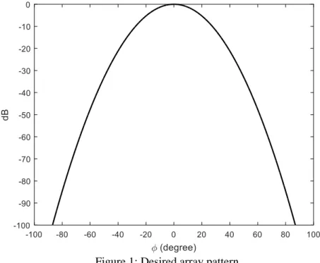
Receiver antenna has been modeled as a circular array consisting of equally spaced eight isotropic elements. The downlink frequency band of the UMTS is between 2110 MHz and 2170 MHz and the corresponding wavelength is between 13.82 and 14.22 cm. We have assumed that the radius of the circular array is equal to 15 cm which is slightly greater than wavelength of the UMTS signal. We have set the frequency that we want to listen to 2110 MHz which corresponds to 14.22 cm wavelength. Pattern of the antenna has been formed with these presumed parameter values by using the method given in [18] in which a cost function depending on square distance between the array far field pattern and the desired pattern has been defined. In order to obtain an array pattern related to the desired pattern one must minimize the cost function with respect to the excitation coefficients of the array elements. A closed form solution to this minimization problem has been given in [18] and calculation of excitation coefficients has been presented. In our study, the desired antenna pattern has been defined by an exponential function
2
0 exp 5 ,
F (3.1) and the pattern is depicted in Fig. 1. The pattern function of an N element circular array in spherical coordinate system O r
, ,
is given in Eq. 3.2 wherea1, ,a , R, and N are excitation coefficients, radius of the circle, and wavelength of the signal respectively
1
, exp sin cos , 2
N k n k F a j R
(3.2)The cost function defining the square distance between desired and the circular array patterns is given in Eq. 3.3.
2 0 0 0 , F F d
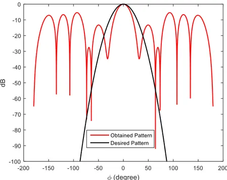
(3.3)where 0 defines a canonical surface. The excitation coefficients have been calculated by minimizing the cost given in Eq. 3.3 using the method given in [18] and the obtained pattern has been presented in Fig. 2. The 3dB
beam width of the desired pattern has been set to around 30 degree and the array pattern calculation came up with approximately 23 degree 3dB beam width which is acceptable in our study.
Figure 1: Desired array pattern
In this study, our aim is to cover 120 degree azimuth sector with the passive radar, and thus we design 10 beams at the receiver site which are obeying the calculated patterns with crossover angle around 6.4 . Target detection in the defined surveillance region is performed over the echoes collected by the formed beams. After obtaining the disturbance free target echo and direct path signal, Matched Filtering is performed. Match filter has an impulse response equal to transmitted waveform (in our case it is direct path signal). When time delayed and frequency shifted version of the transmitted signal (echo form the target) applied to the input of the filter, the output would give maximum the signal-to-noise ratio where time and frequency shifts are matched. Magnitude of the matched filter output is also known as the cross-ambiguity function which is simply Fourier transform of the correlation of the direct path signal and target echo. Cross ambiguity function constitutes range-Doppler map on where the detection process will be performed. Generic detection process is
shown in Fig. 3. Target detection is performed by using Constant False Alarm Rate (CFAR) algorithm. CFAR detection provides predictable detection and false alarm behavior in realistic interference scenarios [7]. To achieve predictive and consistent detection performance with desired false alarm rate, actual interference power must be estimated from data in real time. As shown in Fig. 3, detection is performed on the Range-Doppler map by testing each cell. When the power of the cell under test exceeds the interference power occurred at that cell then, detection is declared. Cell Averaging CFAR (CA-CFAR) technique estimates the interference power at the cell under consideration as the sample mean of the adjoining cells. If there is an echo in a cell exceeding the threshold, a detection is declared and the measurement (plot) belonging to this echo is extracted as the collection of bistatic range, range-rate (negative of Doppler frequency times wavelength), and azimuth with respect to the receiver. Azimuth measurement is obtained by using sequential lobing technique where simply the sum and difference signal powers of two neighboring beams are processed to find the direction of the signal.
Match Filter Output: Complex
Range-Doppler Cells
The cell under test Range D o p p ler Range-Doppler Map Cross Ambiguity Function | . | Thresholding Figure 3: Generic detection process.
4. TARGET TRACKING ALGORITHM
In this study, we aim to track the state of the targets in 2D Cartesian space by using the measurements extracted by the UMTS passive radar. A tracking algorithm similar to one given in [7] has been implemented and its high level block diagram has been given in Fig. 4. The implemented tracking algorithm has two stages where bistatic domain processing is followed by the Cartesian domain processing. Track initiation, measurement to track association is only performed in bistatic domain whereas state estimation (filtering) is carried out both in bistatic and Cartesian domain. An important point must be stressed here, that only the confirmed tracks, which are still alive after a certain track initiation rule, are tracked in Cartesian space. The reasons behind separating the tracking process into two domain are as follows: The range and range-rate measurements are the function of the
travelling time of the transmitted signal in 3D Cartesian space, If the elevation information of the target is not available, one can only
estimate the target state in 2D Cartesian space,
Track initiation and measurement to track association processes involve conversion between bistatic and Cartesian spaces, where bistatic measurements are originating form 3D Cartesian space and target state is defined in 2D Cartesian space,
Since the error arising from the conversion between measurement domain and domain of state will lead to false or no measurement association, then track initiation and as consequence target tracking cannot be accomplished.
The problem explained above can be addressed by separating tracking into two stage as shown in Fig 4. A track begins its life in bistatic domain where measurement and the state have a linear relation, measurement to track
association is performed in here, and maintenance of the confirmed tracks are carried out in both bistatic and Cartesian domain.
Confirmed Tracks Tentative Tracks Measurements
Tracking in Bistatic Domain (Kalman Filter) & Measurement to Track Association & Track Initiation
Tracking in Cartesian Domain (Unscented Kalman Filter)
Estimation / Measurement Updated Tracks (Bistatic) Updated Tracks (Cartesian) Information of Cartesian Tracks Information of Bistatic Track and Measurements
Figure 4: Block diagram of the tracking algorithm.
State estimation under linear dynamic and measurement equation can be performed by using Kalman filter. Kalman filter is the optimal filter in terms of minimum mean square error under linear Gaussian assumptions and it is the best linear estimator if the noise sequences are not Gaussian. Since, measurements and state have linear relation in bistatic domain and the Kalman filter gives the best estimation, preforming initiation and measurement to track association in bistatic domain would lead to better performance in comparison to Cartesian domain.
Target state vector in bistatic domain has been modeled as
T B
k k k k k k
x R R R (4.1)
where subscript k indicates time index, and the superscript B and T are bistatic domain indicator and vector transpose respectively. Bistatic state has been modeled as evolving in time with respect to dynamic equation given in Eq. 4.2,
1 , 0,1,
B B
k k k k
x F x k (4.2)
where F is the state transition matrix, and kis the noise sequence with zero mean and covariance Q . State transition matrix and process noise covariance k are defined as the function of the time difference T , i.e., the time is elapsing k between the previous measurement and current one. F and Q are given in Eq. k 4.3, and q and qR are process noise intensity for range and azimuth respectively.
5 4 3 4 3 2 3 2 3 2 2 1 1 1 0 0 20 8 6 1 1 1 1 0, 5 0 0 0 0 8 3 2 0 1 0 0 1 1 , 0 0 1 0 0 0 0 6 2 0 0 0 1 1 1 0 0 0 0 0 0 0 1 3 2 1 0 0 0 2 R k R k R k k k R k R k R k k k k R k R k R k k k k k k q T q T q T T T q T q T q T T F Q q T q T q T T q T q T q T q T (4.3)
The passive radar has modeled in this paper is capable of measuring bistatic range, range-rate, and azimuth which are linear function of the state vector B
k x
. Hence, the measurement equation can be written as follows:
1 1 1
B
k k k
z Hx (4.4)
In Eq. 4.4, H is the measurement matrix and given in Eq. 4.5, and k1is the zero mean measurement noise sequence with covariance k1.
1 0 0 0 0 0 1 0 0 0 0 0 0 1 0 H (4.5)
Kalman filter in bistatic domain has been designed by using the state space model defined in Eq. 4.2–4.5 and initiated as follows: Assume that at time k, there are M tentative and confirmed targets, and N new measurements which could not have been associated with the existent tracks. Each new measurement would generate a new track with initial estimation B j,
k
x and
covariance j k
P , jN 1, ,M . A Kalman filter would be assigned to each track and initial estimation and covariance of the filter have been given in Eq. 4.6. Each new track is considered as a tentative track and its situation, i.e., updated with measurement in the subsequent scans, is observed. If a tentative track passes a certain test based on updating with measurement in consecutive scans, it is considered as a confirmed track and its state is tracked both in bistatic and Cartesian domain. The test applied to each tentative track is known as track initiation rule and we have implemented 2/2 and m out of n initiation rule, that is, when a track shows up first time its state must be updated with measurement in the following scans, and m update with measurement has to be occurred in next n scans.
, 2 2 2 2 2 2 2 2 2 2 0 0 , m 0 0 0 0 0 m s 0 0 0 0 0 1 m s 0 0 0 0 0 rad 0 0 0 0 0 48 rad s i k i k i k T T B j i i i i i i i k k k k k k k k R R j k x R R z R R P (4.6)Measurement to track association problem has been also solved in bistatic domain. The problem has been modeled as 2D assignment problem where miss detection, and the measurement is originated from the clutter cases have been also taken in to account. This problem consists of finding the best target – measurement matching with respect to minimizing a cost or maximizing a profit function. An assignment matrix has been calculated by using the likelihoods between targets and measurements sets, then, the measurement to target assignment solution giving the maximum profits has been computed by Auction algorithm.
As mentioned before, confirmed tracks are filtered both in bistatic and Cartesian domain. Filtering in bistatic domain provides measurement to track association and Cartesian domain filtering yields solution to the nonlinear stochastic equations which can be interpreted as a mapping form bistatic domain to 2D Cartesian domain. Since the measurement of the passive radar is nonlinear function of the Cartesian state vector, we have implemented unscented Kalman filter. UKF is a well-known target tracking algorithm that provides approximate solution to first and second moments of the state’s posterior density by transforming deterministically selected points through the nonlinear functions. When a track becomes a confirmed track, UKF must be initiated by calculating its initial estimation and covariance. We have modeled target state vector in Cartesian space as
T C
k k k k k
x x x y y (4.7)
where superscript C and subscript k indicate the Cartesian space and time respectively. Assume that location of the transmitter and receiver are
xT,yT
and
xR,yR
respectively, and the associated measurements with the ith tentative track at time k1 and k are 1 1 1 1T
k k k k
z R R and
T
k k k k
confirmed, then the measurements obtained in the last two consecutive scan are transformed into 2D Cartesian space according to Eq. 4.8–4.10.
, if , if k RT k RT k RT k k RT (4.8)
2 2 2 cos k r k k k R L R R L (4.9) cos , if 2 cos , otherwise sin , if 2 , otherwise r k k R k k r k k r k k R k k r k R R x x R R y y R y (4.10)The angles given in Eq. 4.8–4.10 are assumed to be measured fr0m the positive X axis in the counter-clock wise direction. The variables RT and L are the angle and distance between receiver and transmitter respectively. After the transform zk1 and z into the 2D Cartesian space, we have evaluated the k initial estimation and covariance as follows:
1 1 6 2 2 2 6 2 2 2 10 m 0 0 0 0 25 10 m s 0 0 0 0 10 m 0 0 0 0 25 10 m s T C k k k k k k k k k C k x x y y x x y T T P (4.11)We have assumed that the state vector C k
x evolves in time with respect to the nearly constant motion model in accordance with Equations 4.12 and 4.13.
1 C C C C k k k k x F x (4.12) Here, C k
is the zero mean process noise sequence with covariance C k Q in Cartesian space.
3 2 2 2 2 1 1 0 0 3 2 1 0 0 1 0 0 0 1 0 0 2 , 0 0 1 1 1 0 0 3 2 0 0 0 1 1 0 0 2 k k k k k C C k k k k k k T T T T T F Q q T T T T T (4.13)
The measurement equation exploited in UKF is described in Equations 4.14 and 4.15.
1 1 1 C k k k z h x (4.14)
2 2 1 1 2 2 1 1 1 1 1 1 1 1 1 1 1 1 1 1 tan k R k R k T k T k k R k k R R C k k k T k k T T k R k R x x y y x x y y x x x y y y R h x x x x y y y R y y x x (4.15)5. SIMULATION AND RESULTS
In this study, a passive radar consisting of single transmitter and single receiver has been modeled and target tracking scheme has been presented. It is assumed that the transmitter is located at
0,3000, 0 m
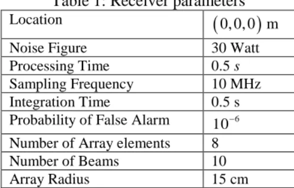
in 3D Cartesian space and transmitted signal obey to the UMTS standards where signal bandwidth is 5 MHz and the transmission frequency is between 2110 MHz and 2170 MHz. The effective radiated power (ERP) of the transmitter is assumed to be 50 Watt. The receiver is modeled as locating at the center ofthe 3D Cartesian space, i.e.,
0, 0, 0 m
, and the parameters of the receiver is given in the Table 1.Table 1: Receiver parameters
Location
0, 0, 0 m
Noise Figure 30 Watt
Processing Time 0.5 s
Sampling Frequency 10 MHz
Integration Time 0.5 s
Probability of False Alarm 6
10 Number of Array elements 8
Number of Beams 10
Array Radius 15 cm
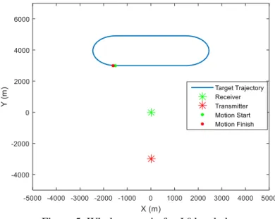
A scenario consisting of a target and clutter has been designed to analyze the performance of the presented tracking scheme. In the scenario, target starts its motion at
1500, 3000, 500 m
with the velocity vector
100, 0, 0 m s
in the 3D Cartesian space. Target moves for 30 seconds according to nearly constant velocity model, then it turns to counter-clock wise direction with constant turn rate 6 deg s during the next 30 seconds. After completing the maneuver, target moves for another 30 seconds with nearly constant velocity, and arrives its initial position by performing another constant turn rate motion with 6deg sturn rate for a 30 seconds. Clutter is also modeled in the scenario where number of clutter per scan is assumed to be a random variable with Poisson distribution and state of the clutter is modeled as a uniformly distributed random variable. In order to analyze the effect of clutter on false track initiation and track continuity, mean number of clutter per scan is modeled in 11 different levels and it is given in Table 2. L0 is the reference level where only the target shows up in the scenario and it is expected to have no false track and maximum track continuity in the simulations. The results obtained with respect to other clutter levels are evaluated in comparison to L0 case. The scenario corresponding to L0 clutter level has been depicted in 2D Cartesian space and given in Fig. 5.Table 2: Mean number of clutter per scan
L0 L1 L2 L3 L4 L5 L6 L7 L8 L9 L10 Mean Number of Clutter per Scan 0 25 50 75 100 125 150 175 200 225 250
Consider the clutter state vector xClutteri belonging to i th clutter in the corresponding scan T i i i i i i i Clutter x x x y y z z
The clutter state vector is modeled to have joint uniform distribution, i.e.,
~ ,
i Clutter
x U a b , and the parameters a and b are define as follows:
5 200 0 200 0 200 5 200 10 200 2 200 T T a km m s km m s km m s b km m s km m s km m s (5.1)Target tracking performance of the UMTS passive radar system has been analyzed through Monte Carlo simulations in terms of number of initiated tracks, track initiation time, track continuity, and the RMS error. In the simulations, input of the Cartesian tracker UKF has been modeled by two ways where in the first one output of the Kalman filter is fed to the UKF as a measurement and in the second one the associated radar measurement in bistatic domain is fed to the UKF.
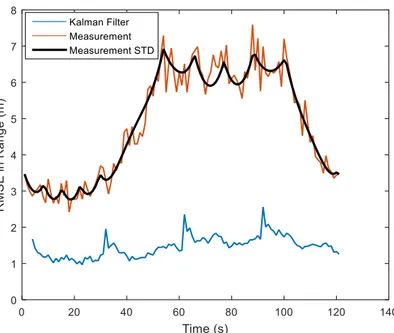
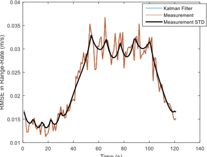
Thus, the effect of using filtered measurements, which are expected to be more accurate, could be analyzed. False track, track initiation time, and track continuity analysis have been carried out with respect to increasing number of clutter and different track initiation logic rules. Three different initiation logic rules, namely 2/2&2/3, 2/2&3/4, and 2/2&4/5, have been implemented for investigating the effects of rule on the number initiated tracks. RMS error evaluation have been only performed in L0 level clutter scenario and tracker performances in both bistatic and Cartesian domain have been presented. Bistatic range, azimuth, and range-rate RMS error results have been depicted in Fig. 6-7-8. The results have been presented in comparison with measurement RMS error and sample mean of the measurement standard deviation calculated by the passive radar. Simulation results have revealed that it is possible to get significant improvement in range and azimuth states by filtering in bistatic domain. Especially in the time interval 50 – 100 seconds, target passes form the furthest region with respect to the passive radar, and hence, measurements can be obtained with lower accuracy due to the small SNR. However, Kalman filter could manage to track target with improving estimation error in range and azimuth as well. The improvement in range state error with respect to the measurement has occurred around 70% at most, and the RMS error of azimuth measurement has been improved around 30% at most. The RMS error result in rate state has showed that range-rate error cloud not be improved and filter tracked the measurements for this state. The reason behind this result can be explained as follows: Since the filter process noise covariance is set to a big value to deal with the measurement to track association problem and passive radar produces highly accurate range-rate measurements due to long integration time, filter gain effecting range-range-rate state increases and the range-rate measurement dominates the range-rate state of the filter output. The RMS error results presented for the Kalman filter are important from the stand point of measurement to track association. Higher accuracy in bistatic tracking leads to smaller estimation covariance which reduces the volume of the association gate while increasing the probability of getting target originated measurement in it. Furthermore, smaller association gate also has benefit of decreasing the probability of clutter being in the gate which reduces the number of false association between measurement and track, and increases the track continuity.
Figure 6: RMS error in bistatic range with average measurement standard deviation
Figure 7: RMS error in azimuth with average measurement standard deviation
Figure 8: RMS error in bistatic range-rate with average measurement standard deviation
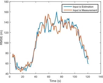
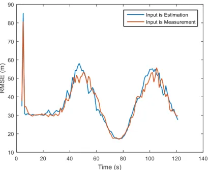
Performance of the UKF has also been analyzed and RMS error results have been depicted in Fig. 9 and 10. As mentioned above, input of the UKF has been modeled to be estimation of Kalman filter or the associated measurement in the bistatic domain. The RMS error results for the both inputs have been given in Fig. 9 and 10, and results have revealed that type of the input does not affect the RMS error in both X and Y axes. This result deserves a bit more attention since the RMS error of the Kalman filter estimate is superior to the measurement error in range and azimuth, but the expected effect of the utilizing more accurate input in the UKF cannot be observed in obtained result. In this state estimation problem, state vector is defined in 2D Cartesian space, but the measuring process is carried out in the 3D Cartesian space, i.e., transmitted signal travels in 3D Cartesian space which leads to obtain time and frequency shift measurements depending on locations and velocities defined in 3D Cartesian space. In the UKF, we assume that the measurements are nonlinear functions of the state vector defined in 2D Cartesian space in the lack of information about target elevation. This misassumption generates a new error source which cannot be modeled in the filter dynamics. Therefore,
projection of the target’s state from 3D to 2D Cartesian space leads to an error depending on the altitude and location of the target. If the target is moving at high altitude and near the receiver and transmitter, then large projection error will be introduced. Since projection errors dominates the UKF estimation error, we have similar RMS error levels while feeding inputs with different accuracies to the UKF. Nevertheless, we have achieved promising result with UKF where RMS error in X axis has been obtained under the 160 m and RMS error in Y axis has been under the 60 m. The difference between RMS errors of X and Y axes arises from the geometry. Since the transmitter and receiver has modeled to be located on the line parallel to the Y axis, the information extracted from measurement about the states related to Y axis is maximized. Therefore, increase in information corresponds to decrease in RMS estimation error.
Performance of the target tracking scheme in the presence of clutter has been analyzed in terms of number of initiated track, track continuity and mean track initiation time. Three different track initiation logic have been implemented and the number of initiated tracks occurred during the tracking has been calculated and depicted with respect to increasing number of clutter in Fig. 11. The “UWE” and “UWM” stand for “Update with Estimation” and “Update with Measurement” respectively. The worst initiated track rate has been obtained with using the track initiation logic 2/2 & 2/3. Approximately 11 tracks is initiated with 2/2 & 2/3 logic rule when the mean number of clutter per scan is 250.
Figure 10: RMS error in Y axis
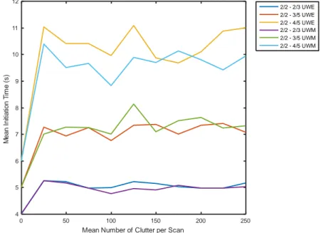
However, the average number of initiated tacks has been less than two for all level of clutter when the other two initiation logic has been utilized. The price of getting smaller number of tracks in the presence of clutter is increase in time that needs to confirm tracks. Mean confirmation times have been shown in Fig. 12. Tracks has been confirmed around in five seconds when 2/2 & 2/3 logic has been utilized. Using 2/2 & 3/5, and 2/2 & 4/5 initiation logic rules has led to track confirmation times around 7 and 10 seconds respectively. Increasing number of clutter affects the track continuity since probability of target’s state being updated with a clutter increases. If the state of a target was updated with clutter in successive scans, target would be lost with high probability. Track continuity performance of the tracking scheme presented in this paper has been shown in Fig. 13. Track continuity is measured in terms of percentage of maximum length of the target originated track that is 121 seconds. Simulation results have revealed that target originated track could be continued at least 82% of its possible life length in all clutter rates. All the results obtained in the presence of clutter has showed that the input of the UKF is irrelevant in terms of defined performance criteria which is consistent with the results obtained in RMS error analysis.
Figure 11: Number of initiated tracks with respect to number of clutter
Figure 12: Mean track initiation times with respect to number of clutter
Mean Number of Clutter per Scan
0 50 100 150 200 250 N u m b e r o f In it ia te d T ra c k 0 2 4 6 8 10 12 2/2 - 2/3 UWE 2/2 - 3/5 UWE 2/2 - 4/5 UWE 2/2 - 2/3 UWM 2/2 - 3/5 UWM 2/2 - 4/5 UWM
Mean Number of Clutter per Scan
0 50 100 150 200 250 M e a n I n it ia ti o n T im e ( s ) 4 5 6 7 8 9 10 11 12 2/2 - 2/3 UWE 2/2 - 3/5 UWE 2/2 - 4/5 UWE 2/2 - 2/3 UWM 2/2 - 3/5 UWM 2/2 - 4/5 UWM
Figure 13: Percentage of track length with respect to number of clutter
6. CONCLUSION
In this paper, we have analyzed appropriateness of UMTS signals for the passive radar applications, and also surveyed performance of the UMTS passive radar by looking from the viewpoint of target tracking. Theoretical calculations have shown that adequate range and Doppler resolution for radar application with high unambiguous range can be achieved. However, low transmission power limits the applicability of the radar to the short ranges. We have presented a two stage target tracking algorithm where track initiation and measurement to track association are performed in bistatic domain and confirmed tracks are filtered in both bistatic and Cartesian domain. Promising results in tracking have been achieved by exploiting two stage tracker where target can be tracked in dense clutter environment with low false track rate and track continuity above 82%. It has also been achieved that false track rate in dense clutter can be decreased by using tighter track initiation logic rule such as 2/2 & 4/5. In the simulations, Cartesian domain filter UKF is updated with two different measurement source which are state estimations of Kalman filter or the measurement exploited to update Kalman filter. Simulation results
Mean Number of Clutter per Scan
0 50 100 150 200 250 L e n g th o f th e T ra c k ( % ) 82 84 86 88 90 92 94 96 98 100 102 2/2 - 2/3 UWE 2/2 - 3/5 UWE 2/2 - 4/5 UWE 2/2 - 2/3 UWM 2/2 - 3/5 UWM 2/2 - 4/5 UWM
have revealed that performance of the UKF is irrelevant of the measurement source, i.e., filter estimation or associated measurement.
REFERENCES
[1] P. Samczynski, K. Kulpa, M. Malanowski, P. Krysik and L. Maslikowski. 2011. A Concept of GSM-based Passive Radar for Vehicle Traffic Monitoring, in Microwaves, Radar and Remote Sensing Symposium, pp. 271-274
[2] D. Petri, F. Berizzi, M. Martorella, E. Dalle Mese and A. Capria. 2010. A Software Defined UMTS Passive Radar Demonstrator, 11th Radar Symposium, pp. 1-4
[3] Y. L. Lu, D. K. P. Tan and H. B. Sun. 2007. Air Target Detection and Tracking Using a Multi-channel GSM Based Passive Radar, in Waveform Diversity & Design Conference, pp. 122-126
[4] H. Sun, D. K. P. Tan and Y. Lu. 2008. Aircraft Target Measurements Using A GSM-Based Passive Radar, IEEE Radar Conference, pp. 1-6 [5] Y. Lu, D. Tan and H. Sun. 2006. An Experimental GSM Based Passive
Radar, in Asia-Pacific Microwave Conference, pp. 1626-1632
[6] P. Krysik, P. Samczynski, M. Malanowski, L. Maslikowski and K. Kulpa. 2012. Detection of Fast Maneuvering Air Targets Using GSM Based Passive Radar, in 19th International Radar Symposium, pp. 69-72 [7] M. A. Richards. 2005. Fundamentals of Radar Signal Processing,
McGraw-Hill
[8] U. R. O. Nickel. 2010. Extending Range Coverage with GSM Passive Localization by Sensor Fusion, 11th International Radar Symposium pp. 1-4
[9] R. Zemmari, B. Knoedler and U. Nickel. 2013. GSM Passive Coherent Location: Improving Range Resolution by Mismatched Filtering, IEEE Radar Conference, pp. 1-6
[10] R. Zemmari, U. Nickel and W. D. Wirth. 2009. GSM Passive Radar for Medium Range Surveillance, in Proceedings of the 6th European Radar Conference, pp. 49-52
[11] R. Zemmari, U. Nickel and W. D. Wirth. 2009. GSM Passive Radar for Medium Range Surveillance, in Proceedings of the 6th European Radar Conference, pp. 49-52
[12] X. Neyt, J. Raout, M. Kubica, V. Kubica, S. Roques, M. Acheroy and J. G. Verly. 2006. Feasibility of STAP for Passive GSM-based Radar, IEEE Conference on Radar, pp.546-551
[13] A. Di. Lallo, A. Farina, R. Fulcoli, P. Genovesi. 2008. Design, Development and Test on Real Data of an FM Based Prototypical Passive Radar, IEEE Radar conference, pp. 1-6
[14] Y. Bar-Shalom, X. R. Li, and T. Kirubarajan. 2001. Estimation with Applications to Tracking and Navigation, Wiley,New York
[15] Y. Bar-Shalom, X. R. Li. 1995. Multitarget-Multisensor Tracking: Principles and Techniques, YBS Publishing
[16] E. A. Wan, R. van der Merwe. 2000. The Unscented Kalman Filter for Nonlinear Estimation, IEEE Adaptive Systems for Signal Processing , Communications, and Control Symposium, pp. 153-158
[17] D. Tan, H. Sun, Y. Lu and W. Liu. 2003. Feasibility Analysis of GSM Signal for Passive Radar, in IEEE Radar Conference, pp. 425-430 [18] R. Vescovo. 1993. Array Factor Synthesis for Circular Antenna
Arrays, Antennas and Propagation Society International Symposium, pp. 1574-1577