Oscillatory flow forced convection in a shallow enclosure with sinusoidal bottom wall temperature

TOBB UNIVERSITY OF ECONOMICS AND TECHNOLOGY INSTITUTE OF NATURAL AND APPLIED SCIENCES

OSCILLATORY FLOW FORCED CONVECTION IN A SHALLOW ENCLOSURE WITH SINUSOIDAL BOTTOM WALL TEMPERATURE

M. Sc. THESIS

Saeid RAHEIMPOUR ANGENEH

Department of Mechanical Engineering

Supervisor: Assoc. Prof. Dr. Murat Kadri AKTAŞ

ii

Approval of the Graduate School of Science and Technology.

……….. Prof. Dr. Osman EROĞUL

Director

I certify that this thesis satisfies all the requirements as a thesis for the degree of Master of Science.

………..

Assoc. Prof. Dr. Murat Kadri AKTAŞ Head of Department

I certify that I have read the thesis named as “Oscillatory flow forced convection in a shallow enclosure with sinusoidal bottom wall temperature” prepared by Saeid RAHEIMPOUR ANGENEH and presented at 11.04.2017, and that in my opinion it is fully adequate in scope and quality, as a dissertation for the degree of Master of Science.

Supervisor: Assoc. Prof. Dr. Murat Kadri AKTAŞ ... TOBB University of Economics and Technology

Examining Committee members:

Prof. Dr. Şenol BAŞKAYA (Chair) ... Gazi University

Prof. Dr. Ünver KAYNAK ... TOBB University of Economics and Technology

iii

TEZ BİLDİRİMİ

Tez içindeki bütün bilgilerin etik davranış ve akademik kurallar çerçevesinde elde edilerek sunulduğunu, alıntı yapılan kaynaklara eksiksiz atıf yapıldığını, referansların tam olarak belirtildiğini ve ayrıca bu tezin TOBB ETÜ Fen Bilimleri Enstitüsü tez yazım kurallarına uygun olarak hazırlandığını bildiririm.

I hereby declare that all the information provided in this thesis has been obtained with rules of ethical and academic conduct and has been written in accordance with thesis format regulations. I also declare that, as required by these rules and conduct, I have fully cited and referenced all material and results that are not original to this work.

iv ABSTRACT

Master of Science

OSCILLATORY FLOW FORCED CONVECTION IN A SHALLOW ENCLOSURE WITH SINUSOIDAL BOTTOM WALL TEMPERATURE

Saeid RAHEIMPOUR ANGENEH

TOBB University of Economics and Technology Institute of Natural and Applied Sciences Mechanical Engineering Science Programme

Supervisor: Assoc. Prof. Dr. Murat Kadri AKTAŞ Date: April 2017

Effects of acoustic streaming on convective heat transfer in a shallow, air-filled, two-dimensional rectangular enclosure with spatially non-uniform temperature distribution of bottom wall are investigated numerically. Excitation of the sound wave in the enclosure is achieved by a periodic motion of the enclosure left wall. The top wall of the enclosure is isothermal while the vertical walls are adiabatic. Compressible form of the Navier-Stokes equations and energy equation are utilized to simulate the flow and temperature fields in the enclosure and solved by Flux Corrected Transport algorithm. Influences of the vibration amplitude and bottom wall temperature profiles are studied. The results demonstrate that the acoustic streaming pattern depends on the temperature profile of the bottom wall and oscillation amplitude. Structure of the flow field in the enclosure affects the rate of heat transfer. The results obtained may have progressive effect on the design of various heat removal applications.

Keywords: Acoustic streaming, Convective heat transfer, Non-uniform temperature profile.

v ÖZET

Yüksek Lisans

SİNÜZOİDAL SICAKLIK DAĞILIMLI ALT DUVARA SAHİP SIĞ KAPALI ALANDA TİTREŞİMLİ AKIŞ YARDIMIYLA ZORLANMIŞ TAŞINIM

Saeid RAHEIMPOUR ANGENEH

TOBB Ekonomi ve Teknoloji Üniversitesi Fen Bilimleri Enstitüsü

Makine Mühendisliği Anabilim Dalı

Danışman: Doç. Dr. Murat Kadri AKTAŞ Tarih: Nisan 2017

Alt duvarın mekansal olarak eşit olmayan sıcaklık dağılımına sahip, sığ, hava dolu, iki boyutlu bir dikdörtgen kapalı alan içerisindeki taşınım ısı geçişine akustik akışın etkileri sayısal olarak incelenmiştir. Kapalı alan içerisindeki ses dalgalarının uyarımı, kapalı alanın sol duvarının periyodik hareketi ile sağlanmaktadır. Kapalı alanın üst duvarı izotermal, dikey duvarları ise adyabatiktir. Sıkıştırılabilir Navier-Stokes denklemleri ve enerji denklemi kapalı ortamdaki akış ve sıcaklık alanlarını modellemek için kullanılmıştır ve Akı-Düzeltmeli Taşınım algoritması ile çözülmüştür. Titreşim genliğinin ve alt duvar sıcaklık profillerinin etkileri incelenmiştir. Sonuçlar, ikinci mertebe girdapların, alt duvarın sıcaklık profiline ve titreşim genliğine bağlı olduğunu göstermektedir. Kapalı ortam içerisindeki akış alanının yapısı, ısı aktarım hızını etkiler. Elde edilen sonuçlar, çeşitli ısı geçişi uygulamalarının tasarımı için yardımcı olabilir.

Anahtar Kelimeler: İkinci mertebe girdaplar, Taşınımlı ısı aktarımı, Düzgün olmayan sıcaklık profili.

vi

ACKNOWLEDGEMENT

I would like to thank Assoc. Prof. Dr. Murat Kadri AKTAŞ, my supervisor who directed me with his valuable help and support, and I also thank to TOBB University of Economics and Technology for providing me scholarship during my education at Mechanical Engineering Department.

I am grateful for the support and prayers of my family, especially my sister. It would be impossible to complete this hard journey without her. I also wish to thank my friends, namely Mustafa Göktürk Yazlak, Sefer Balcı, Berk Çevrim, Eylül Çetindağ and Zehra Oluz, who were very generous in helping me in every step of the study as well as hard times of the life that can happen to all of us.

I would like dedicate my work to my beloved father who taught me every value of life, work, humanity and honor.

vii INDEX Page TEZ BİLDİRİMİ ... iii ABSTRACT ... iv ÖZET ... v ACKNOWLEDGEMENT ... vi INDEX ... vii

LIST OF FIGURES ... viii

LIST OF TABLES ... x

ABBREVIATIONS ... xi

1. INTRODUCTION ... 1

1.1. Literature Review ... 3

1.1.1. Analytical and numerical investigations ... 3

1.1.2. Experimental investigations ... 6

1.1.3. Effects of variable wall temperature on natural convection... 9

1.2. Research Needs ... 10

2. PROBLEM DESCRIPTION AND MATHEMATICAL MODEL ... 11

2.1. Governing Equations ... 12

2.2. Computational Technique ... 14

2.3. Initial and Boundary Conditions ... 18

3. RESULTS………..21

3.1. Second-order Vortices Induced by Vibrating Left Wall ... 21

3.2. Influence of the Non-uniform Temperature Profile on Streaming Structures and Associated Heat Transfer ... 34

4. CONCLUSION ... 59

REFERENCES ... 61

viii

LIST OF FIGURES

Page Figure 1.1 : Standing wave patterns at various frequencies of oscillation. ... 1 Figure 1.2: Schematic of the inner and outer streaming rolls [2]... 2 Figure 2.1: Schematic view of the problem. ... 11 Figure 2.2: Viscosity and thermal conductivity of air as a function of temperature. . 13 Figure 2.3: 101×101 numerical mesh. ... 16 Figure 2.4: Flow chart of FCT scheme [22]. ... 17 Figure 3.1 : Velocity distributions in the enclosure during 40th acoustic cycle at four

instants for Case A: (a) t=/2, (b) t=, (c) t=3/2 and (d) t=2. .. 22 Figure 3.2 : Distribution of (a) pressure and (b) x-component of the velocity along

the horizontal mid-plane (y=H/2) of the enclosure during the 40th cycle for Case A at t=/2, t=, t=3/2, and t=2. ... 24 Figure 3.3 : Pressure contours in the enclosure during the 40th cycle for Case A at: (a)

t=/2, (b) t=, (c) t=3/2 and (d) t=2. ... 25 Figure 3.4: Time-averaged flow field in the enclosure at t=0.04 s for Case A. ... 26 Figure 3.5: Time-averaged flow field in the enclosure at t=0.04 s for: (a) Case B and

(b) Case C. ... 27 Figure 3.6: Non-dimensional streaming velocity profile along the semi height of the

enclosure; (a) x-component at x=3L/4 and (b) y-component at x=L/2. .. 28 Figure 3.7 : Variation of the x-component of the acoustic streaming velocity along a

vertical line at x=L/4 for Case A with different mesh structures. ... 29 Figure 3.8: Distribution of the x-component of the streaming velocity for Case A, B

and C along the vertical lines at (a) x=L/4 and (b) x=3L/4. ... 30 Figure 3.9 : Distribution of the y-component of the streaming velocity for Case A, B

and C along the vertical line at x=L/2. ... 31 Figure 3.10: Temporal variation of the pressure on the mid-point of the right wall for

Case A during (a) all periods and (b) last two periods. ... 32 Figure 3.11: Temporal variation of the pressure on the midpoint of (a) left and (b)

right walls for Case A, B and C during the 40th acoustic cycle. ... 33 Figure 3.12: Temporal variation of the x-component of the velocity on the midpoint

of the enclosure during the last four periods. ... 34 Figure 3.13: Streaming flow field in the enclosure at t=0.04s for (a) Case A-1 and (b) Case A-3. ... 36 Figure 3.14: Variation of the x-component of the streaming velocity at t=0.04 s along the y-axis at (a) x=L/4 and (b) x=3L/4. ... 37

ix

Figure 3.15: Cycle-averaged density profile along the enclosure height at t=0.04 s for Case A, A-1 and A-3 at (a) x=L/4 and (b) x=3L/4. ... 38 Figure 3.16: Streaming flow field for half-sinusoidal cases. ... 40 Figure 3.17: Streaming flow field for sinusoidal cases. ... 41 Figure 3.18: Temporal variations of the pressure on the midpoint of the right wall for

Case A, A-1, A-2, A-3 and A-4 around the 40th acoustic cycle. ... 42 Figure 3.19: Distribution of the axial primary velocity along the enclosure length at

y=H/2 at=t=/2 during the 40th acoustic cycle. ... 43 Figure 3.20: Cycle-averaged temperature contours at t=0.04 s for (a) Case A-1, (b)

Case A-2, (c) Case A-3 and (d) Case A-4. ... 44 Figure 3.21: Evolution of the spaced-averaged Nusselt number with time at (a)

bottom and (b) top walls during the last period for Case A-3, B-3 and C-3. ... 45 Figure 3.22: Pressure contours in the enclosure during the 40th cycle for Case A-3 at:

(a) t=/2, (b) t=, (c) t=3/2 and (d) t=2. ... 46 Figure 3.23: Temperature contours in the enclosure during the 40th cycle for Case

A-3 at: (a) t=/2, (b) t=, (c) t=3/2 and (d) t=2. ... 47 Figure 3.24: Variation of the average Nusselt number with the modified Eckert

number at the bottom and top walls. ... 49 Figure 3.25: Variation of the non-dimensional streaming velocity gradient with the

modified Eckert number at the bottom and top walls. ... 50 Figure 3.26: Variation of the y-component of the streaming velocity along the

enclosure height for half-sinusoidal cases at (a) x=L/2 (TBmax=310 and

320 K), (b) x=L/8 and 7L/8 (TBmax=310 K) and (c) x=L/8 and 7L/8

(TBmax=320 K). ... 51

Figure 3.27: Variation of the y-component of the streaming velocity along the enclosure height for sinusoidal cases at (a) x=L/8 and 7L/8 (TBmax=310

K) and (b) x=L/8 and 7L/8 (TBmax=320 K). ... 52

Figure 3.28: Time-averaged flow field in the enclosure for (a) Case 1, (b) Case B-2, (c) Case C-1 and (d) Case C-4 at t=0.04 s. ... 53 Figure 3.29: Temporal variation of the heat rate from the bottom wall for cases with

Xmax =60 µm for (a) all periods and (b) last ten periods. ... 55

Figure 3.30: Temporal variation of the heat rate from the bottom wall for cases with Xmax =80 µm for (a) all periods and (b) last ten periods. ... 56

Figure 3.31: Temporal variation of the heat rate from the bottom wall for cases with Xmax =100 µm for (a) all periods and (b) last ten periods. ... 57

x

LIST OF TABLES

Page Table 3.1 : Cases simulated. ... 21 Table 3.2 : Cases considered. ... 35 Table 3.3 : Cases with intermediate temperatures. ... 39 Table 3.4 : Rayleigh streaming velocity, Reynolds number and modified Eckert

number of cases. ... 48 Table 3.5 : Local heat fluxes at x=L/8, L/2 and 7L/8 for cases studied. ... 54

xi

ABBREVIATIONS

PIV Particle Tracking Velocimetry LDV Laser Doppler Velocimetry FCT Flux-Corrected Transport

xii

LIST OF SYMBOLS

The symbols used in this study are presented below along with their explanations.

Symbols Explanation

c Speed of sound

cp Specific heat at constant pressure

cv Specific heat at constant volume

E Ec Total energy Eckert number f Frequency H Enclosure height k Thermal conductivity L Enclosure length p Pressure q Heat rate R Ra

Ideal gas constant Rayleigh number

Re Reynolds number

Nu Nusselt number

t Time

T Temperature

u Axial component of velocity

v Transverse component of velocity

x x coordinate y y coordinate  Wavelength  Dynamic viscosity  Kinematic viscosity   Density Angular frequency

1 1. INTRODUCTION

Interference of two sinusoidal waves with the same amplitude and wavelength which move in the opposite directions leads to a standing wave [1]. Some points on the standing wave do not oscillate at all. These points are called nodes. Some points have the largest amplitudes and are named as antinodes. These points are the locations on the standing waves at which the fluid has the largest and smallest values of its properties such as pressure and velocity. Figure 1.1 presents the standing waves made with oscillation of a vibrator at different frequencies.

Figure 1.1 : Standing wave patterns at various frequencies of oscillation.

Standing waves are set up at certain values of the oscillation frequencies which are called resonant frequencies. If the vibrator oscillates at a frequency different than a resonant frequency, standing wave is not established. The relation between 𝜆 (wavelength), 𝑓 (resonant frequency), 𝑣 (speed of travelling wave) and L (fixed distance) is given by:

𝑓 =𝑣 𝜆 = 𝑛

𝑣

2

Mechanical vibrations can produce standing sound waves. Presence of the standing sound waves in a channel filled with viscous fluid induces steady cellular motion of the fluid (acoustic streaming) due to the interaction between the acoustic wave and solid boundaries. These second order, rotational, steady streaming vortices can be classified into three groups as Rayleigh, Schlichting and Eckert streaming.

Schlichting streaming (inner vortices): Inner vortices are formed at the vicinity of the solid boundaries due to the viscous forces and their sizes (in transverse direction) can be determined by the acoustic boundary layer thickness, namely 1.9𝛿. The acoustic penetration depth is defined as

𝛿 = (

𝜔

)

𝜔 is the angular frequency.

Rayleigh streaming (outer vortices): This type of the vortices forms outside the boundary layer and have greater size relative to the inner streaming. The outer vortices have a 𝜆/4 periodicity and fill the half of the channel approximately.

Eckert streaming: This kind of streaming appears in travelling acoustic wave fields. The formation mechanism of Eckert streaming is completely different than inner and outer streaming.

In this study Rayleigh and Schlichting streaming are considered. Figure 1.2 illustrates the outer and inner streaming rolls.

3

Acoustic streaming plays important roles in many applications such as acoustic compressors, thermos-acoustic coolers, ultrasonic surface cleaning and heat exchangers. These second-order vortices affect the heat transfer. Increasing the heat transfer with second order vortices is especially important in areas where the heat transfer with other modes is difficult. For example, acoustic streaming can be used as an aid to heat transfer in such an environment, with low or no gravity since there is no heat transfer by natural convection in these environments. In order to use this technology with all its advantages, it is necessary to understand the nature of acoustic streaming and the associated heat transfer.

1.1. Literature Review

1.1.1. Analytical and numerical investigations

The first theoretical work on acoustic-induced second order vortices was made by Lord Rayleigh [3]. Lord Rayleigh studied the flow of vortices in case of a longitudinal sound field in a Kundt tube. Rayleigh worked on outer vortices and the results found were independent of the viscosity of the fluid. Schlichting [4] considered an incompressible oscillating flow over a flat plate and investigated the patterns of the streaming inside the boundary layer.A general vorticity equation was obtained by Westervelt [5], and a method to evaluate the streaming velocities generated by standing sound wave was developed.

Andres and Ingard [6, 7] studied acoustic streaming formed around a cylinder for both low and high Reynolds numbers (𝑅𝑒 =𝑈0𝑅

 where 𝑈0 stands for the particle

velocity, 𝑅 is the cylinder radius and  represents the kinematic viscosity), analytically. It is revealed that the flow structure formed around the cylinder at high Reynolds number has opposite direction compared with the low Reynolds number case.

Kurzweg [8] investigated the heat transfer driven by the sinusoidal oscillatory flow between two reservoirs which maintained at different temperatures and connected to each other by series of circular tubes, analytically. The influence of oscillation amplitude, frequency, Prandtl number and tube diameter on heat transfer is revealed.

4

Qi worked theoretically on the effect of compressibility on acoustic flow near a solid boundary [9]. It was emphasized that compressibility was a necessary condition for the propagation of acoustic waves, but previous studies were limited to incompressible flow. It is found that compressibility causes high flow velocities outside the boundary layer. Qi and his group [10] investigated the streaming created by acoustic activation in a long wide cylinder, by adding compressibility and heat conduction in their calculations. They analyzed the second order vortices inside the boundary layer. It is found that the x-component of the streaming velocity is a function of compressibility, Prandtl number and specific heat ratio.

Vainstein et al. [11] studied the heat transfer in presence of sound wave between two parallel horizontal flat plates maintained at different temperatures, theoretically. An acoustic Peclet number was defined. In addition, an average Nusselt number based on the Peclet number was derived. Their analysis shows that the existence of a sound field with high frequency and amplitude, affects the heat transfer.

Guo and Sung [12] performed a computational investigation to carry out the effects of oscillating flow on heat transfer in a pipe. Pulsation amplitude of the flow and Womersley number (𝛽 = 𝑎(𝜔⁄ )_ 1/2 _{where 𝑎 is the pipe radius, 𝜔 indicates the}

angular frequency and  is the kinematic viscosity) were used to characterize the flow. Both augmentation and reduction in the heat transfer contingent on the Womersley number are observed for small values of the oscillating amplitude. However heat transfer is always enhanced as a result of high amplitude oscillatory flow.

Effects of oscillatory flow on heat transfer in a pipe in which pipe wall was exposed to constant heat flux were studied analytically by Moschandreou and Zamir [13]. Influences of Prandtl number and oscillation frequency on the heat transfer rate were carried out. It is found that, the rate of heat transfer from wall increases in a certain range of a frequency and reduces out of this range. The rate of heat transfer is augmented with decreasing Prandtl number.

An analytical solution was derived by Hamilton et al. [14] for the streaming which was produced by shaking a two-dimensional rectangular resonator in the x-direction. The essential limitation in this study is that the acoustic wavelength is too larger than oscillatory boundary layer thickness. It is found that the size of the inner vortices

5

decrease as the wide of the channel is increased. Hamilton et al. [15] extended their work by including the thermal effects in calculations which were also applied for cylindrical tubes. It is reported that the streaming velocities are impressed by a few percent due to the effect of heat conduction and temperature dependent viscosity in both very wide and narrow channels. It is also found that in channels of intermediate widths (10-20 times of the boundary layer thickness) thermal conductivity has a considerable effect on acoustic streaming. The results of the cylindrical tubes analysis are the same with the two dimensional channels.

Kawahashi and Arakawa examined the acoustic streaming in an air-filled rectangular enclosure where the standing sound wave was established by the sinusoidally motion of a piston at one end of the duct [16]. Both the first and second order velocities depend on the amplitude of the oscillation. As the amplitude of vibration increases, deformation in the structure of streaming rolls is observed.

Frampton et al. [17, 18] studied the structure of acoustic streaming in micro-fluidic devices analytically. A cylindrical channel with infinite long rigid walls was considered in which one end was subjected to a longitudinal acoustic wave. It is revealed that with reduction in the channel height, the boundary layer streaming becomes dominant while the mean flow velocity remains unchanged. The obtained results show that the acoustic streaming may be effective in micro-fluid control applications.

Aktas and Farouk [19] numerically examined the formation of the second-order vortices produced by acoustic vibration in a rectangular enclosure filled with compressible gas. The sound field in the resonator was induced by the harmonic motion of the enclosure left wall. In this research, effects of the vibrating wall displacement and the enclosure height on the vortex structures were investigated. To obtain Rayleigh streaming structure (streaming rolls have a 𝜆 /4 periodicity), the maximum displacement of the oscillating wall must be reduced as the enclosure height increases. Reduction in the left wall displacement amplitude cannot form the regular Rayleigh streaming in the wide resonators (H/L=0.14 where H and L indicate the enclosure height and length). The greater height and wall displacement increase the number of streaming cells.

6

Carlsson et al. [20] studied the streaming pattern in an incompressible fluid, enclose between two infinite long parallel plates which vibrate in transverse direction, theoretically. They examined the streaming structure in terms of two parameters: frequency and channel height. Four different types of streaming flows depend on these parameters are formed in the channel.

Heat transfer from a rigid wall subjected to sinusoidal temperature profile with an oscillatory flow was studied by Ramos et al. [21]. They assumed incompressible flow with uniform axial velocity. It is found that the heat transfer from the wall remains zero for different values of oscillating velocity amplitudes.

A numerical investigation was carried out to study the effect of acoustic streaming on convective heat transfer in an air filled rectangular enclosure in which the horizontal walls were kept at different temperatures by Aktas and Ozgumus [22]. The results demonstrate that the transverse temperature gradients have significant influence on streaming patterns. The streaming structure formed in the resonator affects the heat transfer.

Daru et al. [23] performed a numerical investigation to study the transition behavior of the acoustic streaming from regular to irregular streaming. They considered a two-dimensional rectangular enclosure filled with air and shaken in the longitudinal direction. It is found that, the presence of the high intensity waves causes to distortion of the streaming rolls and the core of the streaming vortices shifts towards the velocity nodes.

Influence of enclosure shape on the accumulation of acoustic streaming was studied numerically by Cervenka and Bednarik [24]. Excitation of the acoustic field in the resonant cavities was achieved by the shaking of the entire body in the longitudinal direction. They considered resonators with three different shapes as rectangular, wedged and elliptical. It is revealed that the structure of the streaming pattern depends strongly on the shape of the resonators.

1.1.2. Experimental investigations

Ro and Loh [25] experimentally examined the influence of the acoustic streaming on convective heat transfer in a gap spaced between a beam and a heated source. The parameters affecting the heat transfer are reported as the vibration amplitude, the gap

7

size and the temperature of the cooled object. With increase of the vibration amplitude and temperature difference between the heated source and working fluid (air), heat transfer is augmented.

Oscillatory air flow created by harmonic and sinusoidal motion of a piston in a closed vertical resonance tube was examined numerically and experimentally by Alexeev et al. [26]. They discussed the effects of adiabatic boundary condition on the flow structure. Temperature of air increases due to the heat generation by shock waves in the tube. As a result, the speed of sound is enhanced and causes to achieve a frequency other than resonance frequency which leads a non-periodic oscillatory flow. However, the results obtained from experimental investigations show that the flow is almost periodic and contradict this theory. With considering isothermal boundary condition, heat interactions induce reduction in pressure amplitude alter the oscillation phase and cause a periodic flow.

Jun et al. [27] investigated the contribution of the oscillatory flow to heat transfer in a pipe, experimentally. They discussed the influence of hydrodynamic parameters and the shape of the resonator on heat transfer. The results demonstrate that the increment in the flow rate and the length of the resonator, increase the heat transfer gradually.

An experimental investigation by using the Laser Doppler Velocimetry (LDA) method was performed to carry out the acoustic streaming formed by a standing acoustic wave in an air-filled cylindrical resonator tube by Thompson et al. [28]. It is found that at comparatively low acoustic amplitudes, the variation of the x-component of the outer second-order velocity along the resonator length is sinusoidal, has parabolic shape along the tube height, and is the quadratic function of the acoustic amplitude. Thompson et al. [29] explored the effects of axial temperature gradient produced thermoacoustically and fluid inertia on the outer streaming with the same experimental technique. As the induced temperature gradient increases, streaming velocity decreases, and considerable deformation in the structure of the streaming roll is observed.

Convective heat transfer induced by acoustic streaming between two horizontal plates studied experimentally and numerically by Hyun et al. [30]. Formation of

8

acoustic streaming in the gap was accomplished by the vibration of the lower beam in the transverse direction while the heated upper beam was kept stationary. They discussed the streaming structure and its effects on the heat transfer. The greater gap size causes reduction in the maximum streaming velocity. However, increment in the vibration amplitude leads to increase in streaming velocity. It is also reported that the considerable temperature drop is achieved in presence of streaming.

Wan et al. [31] studied the influence of the acoustic streaming on convective heat transfer in a narrow channel filled with air, computationally and experimentally. Streaming flow field in the channel was established by vibration of the bimorph in y-direction. The upper beam was stationary with heat source attached. Particle Tracking Velocimetry (PIV) method was used in the experimental procedure. It is revealed that the induced acoustic streaming augments the heat transfer from the heated source to the air. Both the numerical and experimental results demonstrate that the acoustic streaming plays an important role in cooling process.

Moreau et al. [32] performed an experiment to analyze the inner and outer streaming cells, generated in an air-filled cylindrical tube via loudspeakers at the two ends of the resonator. Measurements of the streaming velocities were achieved by using Laser Doppler Velocimetry (LDV) method. In order to characterize the streaming, the Reynolds number (𝑅𝑒 = (𝑈_𝑐)2₍𝑅

𝛿)2 where U is the acoustic velocity amplitude, R

is the radius of the tube, c denotes the speed of sound, and 𝛿 is the acoustic penetration depth) with wide range was consumed. Reduction in the normalized axial second order velocity is observed near the middle section of the tube with increasing of the Reynolds number. It is also reported that at the Reynolds number approximately equal to 70 two additional streaming vortices appear at the vicinity of the enclosure wall.

An experimental investigation performed by Nabavi et al. [33] to study of the regular and irregular acoustic streaming in an air-filled rectangular enclosure by using Particle Tracking Velocimetry (PIV) technique. They used streaming Reynolds number (𝑅𝑒 = 1/2(𝑢𝑚𝑎𝑥

𝑐 )2( 𝐻

𝛿)2 where 𝑢𝑚𝑎𝑥 and c denote the maximum acoustic

velocity in the enclosure and the speed of sound, H is the resonator height and 𝛿 is the acoustic penetration depth) to classify the regular and irregular streaming. It is revealed that when the steaming Reynolds number is greater than 50, the regular

9

streaming patterns distort and the complex shapes are formed. In other work, Nabavi and his group [34, 35] studied the effects of horizontally heated walls on streaming structure in an air-filled resonant cavity with PIV method again, experimentally. Presence of the transverse temperature gradient deforms the symmetric shape of the streaming and leads to increment in the streaming velocity.

Reyt et al. [36] performed both experimental and numerical analysis to investigate the formation of acoustic streaming, generated by shaking of an air-filled cylindrical resonator. They used LDV method in the experimental study and considered the compressible form of the Navier-Stokes equations in the numerical analysis. It is found that the cores of the outer streaming rolls are pushed towards the acoustic velocity nodes and new streaming vortices formed in the vicinities of the acoustic velocity antinodes as the Reynolds number (𝑅𝑒 = (𝑈_𝑐)2₍𝑅

𝛿)

2_{) increases.}

Tajik et al. [37] studied the influence of acoustic streaming on heat transfer from a heated source located at the top of the water-filled cylindrical enclosure, experimentally. Standing wave in the enclosure was established by the vibration of the bottom plate in the transverse direction with the aid of ultrasonic transducer. The results obtained shows that in presence of acoustic streaming, heat transfer can be improved by about 390%. It is also found that the heat transfer increases as the distance between the heat source and vibrating plate reduces at a given ultrasonic power. Increase in the ultrasonic power also leads to augmentation in heat transfer.

1.1.3. Effects of variable wall temperature on natural convection

Influence of temperature oscillations on natural convection boundary layer near a cylindrical surface studied theoretically by Merkin and Pop [38]. The obtained results show that, in oscillations with high frequency and large times, a steady flow is formed outside the boundary layer.

A numerical investigation of free convection in an enclosure with spatially sinusoidal temperature distribution of heated wall was carried out by Saeid [39]. It is found that length of heat source and amplitude of the sinusoidal temperature profile affect the heat transfer in the cavity. Augmentation in average Nusselt number is observed as the heat source length or temperature profile amplitude increases.

10

Bilgen et al. [40] investigated the laminar natural convection in an enclosure of which one side wall was exposed to sinusoidal temperature profile, numerically. It is found that, thermal penetration strongly depends on the Rayleigh number and enclosure aspect ratio.

Varol et al. [41] studied the natural convection in a rectangular enclosure in which, bottom wall subjected to spatially sinusoidal temperature profile, numerically. It is revealed that increase in the aspect ratio of the enclosure causes reduction in heat transfer. As the amplitude of temperature profile increases, heat transfer is enhanced.

Wang et al. [42] studied the transient natural convection between two infinite horizontal walls with sinusoidally oscillating temperature profiles, numerically. Time-averaged heat flux from the lower to the upper wall is observed even though the time-average temperature difference between walls is zero. The same result was obtained for different values of temperature oscillation frequency, Grashof number and the distance between walls.

1.2. Research Needs

None of the investigations in the literature considered the influence of non-uniform temperature profiles on the acoustic streaming and associated heat transfer. Thus this study mainly focuses on the influence of the non-uniform temperature profile on the streaming pattern and corresponding heat transfer. To the best of authors’ knowledge, this is the first examination of the influence of nonzero mean vibrational flow on the thermal convection from a surface with non-uniform temperature distribution. The results obtained may have useful effect on the design of various heat removal applications.

11

2. PROBLEM DESCRIPTION AND MATHEMATICAL MODEL

A two-dimensional rectangular resonator filled with air is considered. In order to produce standing wave, the left wall of the enclosure vibrates in the longitudinal direction with lowest resonant frequency. Both horizontal and side walls are rigid. The schematic view of the problem is presented in Figure 2.1.

Figure 2.1: Schematic view of the problem.

The harmonic displacement and velocity of the vibrating wall are given by:

𝑥(𝑡) = 𝑥𝑚𝑎𝑥sin(𝜔𝑡) (2.1)

𝑢(𝑡) = 𝜔𝑥_𝑚𝑎𝑥cos(𝜔𝑡) (2.2)

Here, 𝑥𝑚𝑎𝑥 symbolizes the maximum displacement amplitude of the left wall and 𝜔

represents the angular frequency, 𝜔 = 2𝜋𝑓. The oscillation frequency is set as 𝑓 = 1 𝑘𝐻𝑧 and related to the wavelength of the sound wave by 𝜆 = 𝑐₀/𝑓 , where 𝑐₀ is the reference speed of sound in air (𝑐0 = 347 𝑚/𝑠). The enclosure length is half of

the wavelength of sound wave, 𝐿 = λ₂= 173.5 mm and the height of the enclosure is 𝐻 = 40𝛿. Here, 𝛿 is the thickness of the acoustic boundary layer and given by

AIR

H

L x

12

𝛿 = √2_𝜔 .The thickness of acoustic boundary layer is approximately 0.07 mm in this

study.

The side walls of the enclosure are adiabatic. The top wall is isothermal and kept at 300 K. The bottom wall of the enclosure is exposed to sinusoidal and half-sinusoidal temperature profiles.

2.1. Governing Equations

The compressible form of the continuity, momentum and energy equations are considered to simulate the flow and temperature fields in the enclosure. In two dimensional Cartesian coordinates, these equations are given as:

𝜕𝜌 𝜕𝑡 + 𝜕(𝜌𝑢) 𝜕𝑥 + 𝜕(𝜌𝑣) 𝜕𝑦 = 0 (2.3) 𝜌𝜕𝑢 𝜕𝑡 + 𝜌𝑢 𝜕𝑢 𝜕𝑥+ 𝜌𝑣 𝜕𝑢 𝜕𝑦= − 𝜕𝑝 𝜕𝑥+ 𝜕𝜏𝑥𝑥 𝜕𝑥 + 𝜕𝜏_𝑥𝑦 𝜕𝑦 (2.4) 𝜌𝜕𝑣 𝜕𝑡 + 𝜌𝑢 𝜕𝑣 𝜕𝑥+ 𝜌𝑣 𝜕𝑣 𝜕𝑦= − 𝜕𝑝 𝜕𝑦+ 𝜕𝜏_𝑦𝑦 𝜕𝑦 + 𝜕𝜏_𝑥𝑦 𝜕𝑥 (2.5) 𝜕𝐸 𝜕𝑡 + 𝜕 𝜕𝑥[(𝐸 + 𝑝)𝑢] + 𝜕 𝜕𝑦[(𝐸 + 𝑝)𝑣] = 𝜕 𝜕𝑥[𝑢𝜏𝑥𝑥 + 𝑣𝜏𝑥𝑦] + 𝜕 𝜕𝑦[𝑢𝜏𝑥𝑦+ 𝑣𝜏𝑦𝑦] −𝜕𝑞𝑥 𝜕𝑥 − 𝜕𝑞_𝑦 𝜕𝑦 (2.6)

In equations above, 𝑡 represents the time, 𝑥 and 𝑦 refer to the Cartesian coordinates, 𝑢 and 𝑣 indicate the velocity components, 𝑝 is pressure and 𝜌 is density. The components of the shear stress, heat flux and total energy are expressed as:

𝜏_𝑥𝑥 =4 3𝜇 𝜕𝑢 𝜕𝑥− 2 3𝜇 𝜕𝑣 𝜕𝑦 (2.7) 𝜏𝑦𝑦 = 4 3𝜇 𝜕𝑣 𝜕𝑦− 2 3𝜇 𝜕𝑢 𝜕𝑥 (2.8) 𝜏_𝑥𝑦 = 𝜇 (𝜕𝑢 𝜕𝑦+ 𝜕𝑣 𝜕𝑥) (2.9) 𝑞_𝑥 = −𝑘𝜕𝑇 𝜕𝑥 (2.10)

13 𝑞𝑦 = −𝑘 𝜕𝑇 𝜕𝑦 (2.11) 𝐸 = 𝑝 𝛾 − 1+ 1 2𝜌(𝑢2+ 𝑣2) (2.12)

Here, 𝛾 is the ratio of specific heats (𝑐_𝑝/𝑐_) and 𝑇 is temperature. The change of dynamic viscosity (𝜇) and thermal conductivity (𝑘) with temperature is followed by the polynomial equations below:

𝜇(𝑇) = −8.73 × 10−7_{+ 8.99 × 10}−8_{𝑇 − 1.09 × 10}−10_𝑇2_{+ 8.3 × 10}−14_𝑇3 _(2.13)

𝑘(𝑇) = −1.97 × 10−3_{+ 1.2 × 10}−4_{𝑇 − 1.09 × 10}−7_𝑇2_{+ 6.79 × 10}−11_𝑇3 _(2.14)

Figure 2.2 compares the viscosity and thermal conductivity values computed with equations above and tabulated values in Incropera [43]. The results are in good agreement.

Figure 2.2: Viscosity and thermal conductivity of air as a function of temperature.

The pressure, density and temperature are related to each other by the ideal gas law:

𝑝 = 𝜌𝑅𝑇 (2.15)

here Rdenotes the specific gas constant.

0.016 0.02 0.024 0.028 0.032 1.2E-05 1.4E-05 1.6E-05 1.8E-05 2.0E-05 2.2E-05 2.4E-05 200 250 300 350 T (K) k ( W /m .K) μ (N .s/ m 2 ) Viscosity (Incropera [43])

14 2.2. Computational Technique

In order to solve the convective part of the equations, an explicit, finite-volume based, Flux-Corrected Transport algorithm is utilized. The diffusion terms are discretized by the central-difference method and added to the solution as a source term. Numerical dispersion and dissipation terms which appear in the numerical scheme result in amplitude and phase errors in the solution. For example in calculations where density is being evaluated, negative density values become visible as a result of oscillations. In order to eliminate or reduce these errors numerical damping terms are added to the calculation process. Consider a numerical scheme in which a damping term is added in a predictor step and a certain amount of damping is removed in a corrector step [44]. Such a numerical scheme is called Flux-Corrected Transport which was developed by Boris and Book [45]. The Flux Corrected Transport (FCT) algorithm is a high-order, non-linear, monotone, conservative, and positivity preserving algorithm developed to solve time-dependent, one-dimensional, nonlinear general continuity equation. This algorithm has fourth order phase accuracy and can solve sharp gradients with minimum numerical diffusion [46].

Consider one-dimensional continuity equation with a three point explicit finite difference formula. Temporary value of density is obtained from the values of previous time step as below:

𝜕𝜌 𝜕𝑡 + 𝜕(𝜌𝑢) 𝜕𝑥 = 0 (2.16) 𝜌̃_𝑖 = 𝜌_𝑖0₋1 2[𝜀𝑖+1₂ (𝜌𝑖+1 0 _{+ 𝜌} 𝑖0) − 𝜀_𝑖−1 2 (𝜌𝑖 0_{+ 𝜌} 𝑖−10 )] + [_𝑖+1 2 (𝜌𝑖+1 0 _{− 𝜌} 𝑖0) − _𝑖−1 2 (𝜌𝑖 0_{− 𝜌} 𝑖−10 )] = 𝜌_𝑖0 − 1 ∆𝑥[𝑓𝑖−1₂− 𝑓𝑖+1₂] (2.17) where 𝑓_𝑖±1

2 indicate inflow and outflow fluxes of density across the cell boundaries.

𝜀_𝑖±1

2 are convective fluxes which are given as:

𝜀_𝑖+1

2 = 𝑢𝑖+12

∆𝑡

15 𝜀_𝑖−1 2 = 𝑢𝑖−12 ∆𝑡 ∆𝑥 (2.19) _𝑖±1

2 are non-dimensional numerical diffusion coefficients.

An anti-diffusion stage of FCT algorithm is defined as: 𝜌_𝑖𝑛 = 𝜌̃𝑖 − 𝑓_𝑖+1 2 𝑎𝑑 _{+ 𝑓} 𝑖−1₂ 𝑎𝑑 (2.20) where 𝑓_𝑖±1 2 𝑎𝑑

are anti-diffusive fluxes and are given as:

𝑓 𝑖−1₂ 𝑎𝑑 _{= 𝜇} 𝑖−1₂ (𝜌̃𝑖 − 𝜌̃𝑖−1) (2.21) 𝑓 𝑖+1₂ 𝑎𝑑 _{= 𝜇} 𝑖+1₂ (𝜌̃𝑖+1− 𝜌̃𝑖) (2.22) here 𝜇_𝑖±1

2 are anti-diffusion coefficients.

Addition of these anti-diffusion fluxes may cause the appearance of a new maximum or minimum in calculation process. In order to prevent these maxima and minima which appear in the anti-diffusive stage, anti-diffusion fluxes are replaced by corrected fluxes as:

𝜌_𝑖𝑛 = 𝜌̃𝑖 − 𝑓_𝑖+1 2 𝑐 _{+ 𝑓} 𝑖−1₂ 𝑐 (2.23)

The corrected fluxes satisfy:

𝑓 𝑖+12 𝑐 _{= 𝑆 ∙ 𝑚𝑎𝑥 {0, 𝑚𝑖𝑛 [𝑆 ∙ (𝜌̃} 𝑖+2− 𝜌̃𝑖+1), |𝑓 𝑖+12 𝑎𝑑_{| , 𝑆 ∙ (𝜌̃} 𝑖− 𝜌̃𝑖−1)]} (2.24)

|S|=1 and its sign is same with the sign of (𝜌̃𝑖+1− 𝜌̃𝑖). If sign of (𝜌̃𝑖+1− 𝜌̃𝑖) is

positive, then corrected flux gives:

𝑓 𝑖+12 𝑐 _{= 𝑚𝑖𝑛 [(𝜌̃} 𝑖+2− 𝜌̃𝑖+1), 𝜇 𝑖+12(𝜌̃𝑖+1− 𝜌̃𝑖), (𝜌̃𝑖− 𝜌̃𝑖−1)] (2.25) or 𝑓 𝑖+12 𝑐 _{= 0} (2.26)

16

whichever is larger. The anti-diffusion flux is inclined to decrease 𝜌_𝑖𝑛 _{and to increase}

𝜌_𝑖+1𝑛 _{. Thus anti-diffusion fluxes cannot produce a new minimum and maximum}

during the calculation process.

Calculations were performed with a one-dimensional LCPFCT (Laboratory for Computational Physics, Flux-Corrected Transport) algorithm [47]. In order to apply this algorithm, the two dimensional continuity, momentum and energy equations are divided into two parts resulting in one dimensional equations in x and y directions. After calculation in x direction is done, computation in y direction is performed. A suitable time step must be chosen in order to satisfy the Courant-Friedrichs-Lewy (CFL=c∆𝑡/∆𝑥) criterion.The CFL number is chosen smaller than 0.4 in both x and y directions in this study. Numerical scheme was developed in FORTRAN language for related calculations. Figure 2.4 represents the calculation procedure in flow chart.

In all simulations, typically a 101 x 101 numerical mesh is used which is shown in Figure 2.3. In order to resolve thin oscillatory boundary layer, the grids are generated non-uniformly in transverse direction and clustered at the vicinity of the horizontal walls. The quality of grids gradually decreases towards to middle section. The grid size is uniform along the longitudinal direction. For each period of the pressure waves emanating from the left wall of the enclosure, 100,000 time steps are used.

17

Figure 2.4: Flow chart of FCT scheme [22]. time ≥

timemax ?

No

Read block data Start

Generate grid - initialize flow variables

Perform FCT procedure in x-direction and update , , and T using computed values of , , ,

Perform FCT procedure in y-direction and update , , and T using computed values of , , ,

Compute diffusion, conduction, viscous dissipation terms, update , , , , , , and T

Update boundary conditions, compute left wall position

Print results

Stop Yes

18 2.3. Initial and Boundary Conditions

The enclosure has no-slip walls. The side walls are adiabatic. A sinusoidal or half-sinusoidal spatial temperature profile is applied to the bottom wall while the top wall is kept at initial temperature. The boundary conditions are:

𝑢(0, 𝑦, 𝑡) = 𝜔𝑋𝑚𝑎𝑥cos(𝜔𝑡) (2.27) 𝑣(0, 𝑦, 𝑡) = 0 (2.28) 𝑢(𝐿, 𝑦, 𝑡) = 𝑣(𝐿, 𝑦, 𝑡) = 0 (2.29) 𝑢(𝑥, 0, 𝑡) = 𝑣(𝑥, 0, 𝑡) = 0 (2.30) 𝑢(𝑥, 𝐻, 𝑡) = 𝑣(𝑥, 𝐻, 𝑡) = 0 (2.31) 𝜕𝑇 𝜕𝑥(0, 𝑦, 𝑡) = 𝜕𝑇 𝜕𝑥(𝐿, 𝑦, 𝑡) = 0 (2.32) 𝑇(𝑥, 0, 𝑡) = 𝑇_𝐵 (2.33) 𝑇(𝑥, 𝐻, 𝑡) = 𝑇𝑇 (2.34)

Sinusoidal and half sinusoidal temperature distributions of the bottom wall are expressed as: 𝑇𝐵= 300 + (𝑇𝐵𝑚𝑎𝑥− 300) sin ( 2𝜋𝑥 𝐿 ) (2.35) 𝑇𝐵 = 300 + (𝑇𝐵𝑚𝑎𝑥− 300) sin ( 𝜋𝑥 𝐿) (2.36)

In order to obtain the density at boundaries properly, an approach recommended by Poinsot and Lee [48] is used along the stationary no-slip walls as:

𝜕𝜌 𝜕𝑡 (𝑥, 0) = − 1 𝑐 𝜕𝑝 𝜕𝑦(𝑥, 0) − 𝜌(𝑥, 0) 𝜕𝑣 𝜕𝑦(𝑥, 0) (2.37) 𝜕𝜌 𝜕𝑡(𝑥, 𝐻) = − 1 𝑐 𝜕𝑝 𝜕𝑦(𝑥, 𝐻) − 𝜌(𝑥, 0) 𝜕𝑣 𝜕𝑦(𝑥, 𝐻) (2.38) 𝜕𝜌 𝜕𝑡(𝐿, 𝑦) = − 1 𝑐 𝜕𝑝 𝜕𝑥(𝐿, 𝑦) − 𝜌(𝐿, 𝑦) 𝜕𝑢 𝜕𝑥(𝐿, 𝑦) (2.39)

19

Since the velocity of the vibrating wall is time-dependent, a modified equation is used to compute the density along the left wall:

𝜕𝜌 𝜕𝑡(0, 𝑦) = 𝛾𝜌(0, 𝑦) 𝑐 𝜕𝑢 𝜕𝑡(0, 𝑦) + 𝛾𝜌(0, 𝑦)(𝑢(0, 𝑦) − 𝑐) 𝑐 𝜕𝑢 𝜕𝑥(0, 𝑦) −𝛾(𝑢(0, 𝑦) − 𝑐) 𝑐2 𝜕𝑝 𝜕𝑥(0, 𝑦) (2.40)

Initial conditions are:

𝑝(𝑥, 𝑦, 0) = 101325 𝑃𝑎 (2.41)

𝜌(𝑥, 𝑦, 0) = 1.1768𝑘𝑔

𝑚3 (2.42)

𝑇(𝑥, 𝑦, 0) = 300 𝐾 (2.43)

The radiation heat exchange between walls in the enclosure is neglected. The particle motion due to free convection occurs in the enclosure when the buoyancy force is large enough, and becomes more important than both viscous forces and thermal diffusion. The critical Rayleigh number for starting motion in the enclosure is about 1708. In this study the maximum value of the Rayleigh number is about 40, and the effect of gravity is neglected also. The Rayleigh number is given by:

𝑅𝑎 =𝑔𝛽∆𝑇𝐻3

𝛼 (2.44)

where 𝑔 is the gravitational acceleration, 𝛽 indicates thermal expansion, ∆𝑇 represents the temperature difference between the walls,  is kinematic viscosity and 𝛼 is thermal diffusivity.

21 3. RESULTS

3.1. Second-order Vortices Induced by Vibrating Left Wall

In this section effect of the maximum displacement of the left wall on oscillatory and mean flow fields is investigated. The bottom wall of the enclosure is kept at 300 K at this section. Table 3.1 lists the cases simulated.

Table 3.1 : Cases simulated.

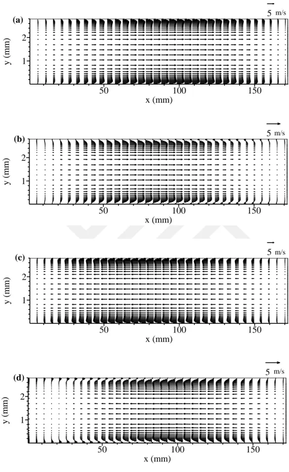
Figure 3.1 shows the oscillatory flow field in the enclosure during the 40th acoustic period at various instants for Case A. These instantaneous flow fields remain same at all periods after 40th acoustic cycle, so the flow is named quasi steady-state. It can be noted that instantaneous velocities in the enclosure change spatially and temporally. Left wall of the enclosure moves through the inside of the enclosure and reaches to its maximum displacement value at 𝜔𝑡 = 𝜋/2 where the flow is towards the right wall. The wall moves back to its initial position at 𝜔𝑡 = 𝜋 while flow is still towards the right wall but slows down. At the instant 𝜔𝑡 = 3𝜋/2, the left wall moves through

the out of the enclosure and reaches to its maximum displacement value and extracts the flow towards itself. The left wall then comes back to its initial position at 𝜔𝑡 = 2𝜋 while the flow is still towards the left wall and slows down. The instant 𝜔𝑡 = 2𝜋 is identical to the instant 𝜔𝑡 = 0 which is the beginning of the next coming cycle. The same pattern can be observed in Case B and C. The maximum values of the x-component of the acoustic velocity in the enclosure reach to 5.5, 7.3 and 9 m/s for Case A, B and C, respectively.

Case 𝑥𝑚𝑎𝑥 (µm) 𝑇𝑇 = 𝑇𝐵 (K)

A 60 300

B 80 300

22

Figure 3.1 : Velocity distributions in the enclosure during 40th acoustic cycle at four instants for Case A: (a) t=/2, (b) t=, (c) t=3/2 and (d) t=2.

x (mm) y (m m ) 50 100 150 1 2 5 m/s

Frame 00108 Feb 2017PLOTF2

x (mm) y (m m ) 50 100 150 1 2 5 m/s

Frame 00108 Feb 2017PLOTF3

x (mm) y (m m ) 50 100 150 1 2 5 m/s

Frame 00108 Feb 2017PLOTF4

x (mm) y (m m ) 50 100 150 1 2 5 m/s

Frame 00108 Feb 2017PLOTF5

(a)

(b)

(c)

23

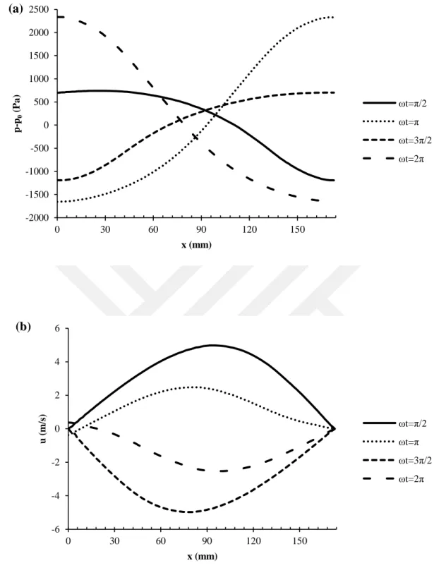
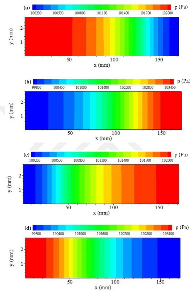
Figure 3.2 represents the distribution of the pressure and the x-component of the velocity along the horizontal mid plane (y=H/2) of the enclosure at four different instants during the 40th acoustic cycle for Case A. The pressure distributions at four various instants of the acoustic cycle indicate that the pressure node forms near the midpoint of the enclosure length (xL/2). The x-component of the velocity at all instants reaches to its maximum value at the same region.

The pressure reaches to its maximum value on the vibrating (left) and minimum value on the stationary (right) wall of the enclosure at t=2 and just the opposite behavior can be observed at t=. A closer look on the Figure 3.2.b shows that, x-component of the velocity at both t=2 and t= changes its sign at the vicinity of the left wall. The flow is towards the left wall along the enclosure length, up to the vicinity of the vibrating wall where the flow velocity changes its sign and flows towards the right wall due to the motion of the vibrating wall to the right at t=2. At this location where the flows with opposite directions collide, the pressure has its maximum value. At t=, the direction of the flow is towards the right wall in the great portion of the enclosure, while it is towards the left near the oscillating wall which moves to the left. At this point where flows with different directions move away from each other pressure gets its minimum value.

Pressure contours in the enclosure at t=/2, , 3/2 and 2 during the 40th cycle for Case A are presented in Figure 3.3. It is obvious that the pressure profiles shown in the Figure 3.2.a remain identical along the any plane from bottom to the top wall in the enclosure.

24

Figure 3.2 : Distribution of (a) pressure and (b) x-component of the velocity along the horizontal mid-plane (y=H/2) of the enclosure during the 40th cycle for Case A at

t=/2, t=, t=3/2, and t=2. -2000 -1500 -1000 -500 0 500 1000 1500 2000 2500 0 30 60 90 120 150 p -p 0 (Pa ) x (mm) ωt=π/2 ωt=π ωt=3π/2 ωt=2π -6 -4 -2 0 2 4 6 0 30 60 90 120 150 u ( m /s) x (mm) ωt=π/2 ωt=π ωt=3π/2 ωt=2π (a) (b)

25

Figure 3.3 : Pressure contours in the enclosure during the 40th cycle for Case A at: (a)

t=/2, (b) t=, (c) t=3/2 and (d) t=2. (a) (b) (c) (d) p (Pa) p (Pa) p (Pa) p (Pa)

26

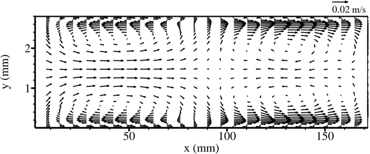
In order to obtain the steady, secondary flow (acoustic streaming) in the enclosure, the time averaged values of instantaneous density, x- and y-components of the velocity (𝑢 and 𝑣) are computed during the 40th

acoustic cycle and the streaming velocities are obtained at t=0.04 s. By this time, quasi steady values are obtained. Further increase of the number of periods has no effect on the computed velocities. Axial and transverse components of the acoustic streaming velocities are represented as 𝑢𝑠𝑡 and 𝑣𝑠𝑡, respectively.

𝑢_𝑠𝑡 =〈𝜌𝑢〉

〈𝜌〉 𝑣𝑠𝑡 = 〈𝜌𝑣〉

〈𝜌〉 (3.1)

The symbol 〈 〉 indicates the time average during one vibration cycle of the enclosure left wall. The streaming pattern in the enclosure for Case A at t=0.04 s is shown in the Figure 3.4. Two types of streaming vortices can be observed in Figure 3.4. The first type is the inner streaming formed near the acoustic boundary layer and the second one is the outer streaming extend from the edge of the inner vortices through the middle section of the enclosure. The outer streaming flows towards the velocity nodes and turns back through the velocity antinode along the horizontal mid-plane to accomplish a closed loop. The inner and the outer streaming rolls have opposite direction of rotation. Both inner and outer streaming vortices are fairly symmetric respect to the horizontal and vertical mid-planes.

Figure 3.4: Time-averaged flow field in the enclosure at t=0.04 s for Case A.

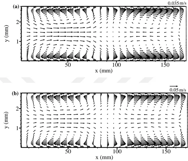
Figure 3.5 represents the streaming flow field in the enclosure at t=0.04 s for Case B and C. While the symmetry of the streaming cells remains unchanged with increase

x (mm) y (m m ) 50 100 150 1 2 0.02 m/s

27

in the maximum displacement of the left wall, the remarkable change in the streaming velocities can be observed.

Figure 3.5 : Time-averaged flow field in the enclosure at t=0.04 s for: (a) Case B and (b) Case C.

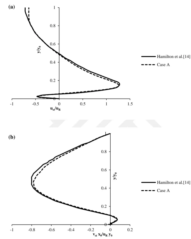
The simulation results are verified with the analytical solution of Hamilton et al. [14]. The x-component (at x=3L/4) and y-component (at x=L/2) of the streaming velocity along the semi-height (y0=H/2) of the resonator for Case A are presented in

the Figure 3.6. A reference streaming velocity uR=3umax2/16c0 is used to normalize

the velocity values. Here umax is the maximum velocity in the oscillatory flow field.

vstx0/uRy0 is the y-component of the non-dimensional streaming velocity. x0 denotes

the semi length of the enclosure (x0 = L/2). The results of the current study slightly

differ from the reference solution. The velocity profiles shown in the reference study are for a resonator where the excitation of the sound field is achieved by shaking the entire enclosure harmonically. However, the resonator under investigation in this

x (mm) y (m m ) 50 100 150 1 2 0.035 m/s

Frame 00109 Feb 2017PLOTF1

x (mm) y (m m ) 50 100 150 1 2 0.05 m/s

Frame 00109 Feb 2017PLOTF1

(a)

28

study is stationary and vibrating a vertical wall produces the sound wave in the enclosure.

Figure 3.6: Non-dimensional streaming velocity profile along the semi height of the enclosure; (a) x-component at x=3L/4 and (b) y-component at x=L/2.

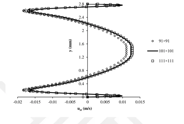
Figure 3.7 illustrates the distribution of the x-component of the acoustic streaming velocity along a vertical line at x=L/4 at t=0.04 s for Case A. In order to show the influence of the grid size on numerical predictions, the results of both coarser

0 0.2 0.4 0.6 0.8 1 -1 -0.5 0 0.5 1 1.5 y /y0 ust/uR Hamilton et al.[14] Case A 0 0.2 0.4 0.6 0.8 1 -1 -0.8 -0.6 -0.4 -0.2 0 0.2 y /y0 vstx0/uRy0 Hamilton et al.[14] Case A (a) (b)

29

(91×91) and denser (111×111) numerical meshes are added to the figure. The results show that the 101×101 numerical mesh is sufficient to solve the flow pattern.

Figure 3.7 : Variation of the x-component of the acoustic streaming velocity along a vertical line at x=L/4 for Case A with different mesh structures.

Variation of the axial component of the second-order velocity along the vertical lines at x=L/4 and x=3L/4 for Case A, B and C are shown in Figure 3.8. Increase in the maximum displacement of the vibrating wall leads to increase in the streaming velocity. In all cases presented here, the symmetric pattern respect to the horizontal mid-plane (y=H/2) can be observed and the classical Rayleigh streaming still exists, although the increment in the maximum displacement of the left wall. Figure 3.9 depicts the distribution of the y-component of the streaming velocity along the enclosure height at x=L/2 for Case A, B and C. The points on the y-axis where the streaming velocity is zero can be considered as the boundary between the streaming rolls. It can be clearly noted that the transverse component of the streaming velocity crosses the y-axis at the same points in all cases.

0 0.4 0.8 1.2 1.6 2 2.4 2.8 -0.02 -0.015 -0.01 -0.005 0 0.005 0.01 0.015 y ( m m ) ust(m/s) 91×91 101×101 111×111

30

Figure 3.8: Distribution of the x-component of the streaming velocity for Case A, B and C along the vertical lines at (a) x=L/4 and (b) x=3L/4.

0 0.4 0.8 1.2 1.6 2 2.4 2.8 -0.05 -0.04 -0.03 -0.02 -0.01 0 0.01 0.02 0.03 0.04 y ( m m ) ust(m/s) Case A Case B Case C 0 0.4 0.8 1.2 1.6 2 2.4 2.8 -0.04 -0.02 0 0.02 0.04 0.06 y (m m ) ust(m/s) Case A Case B Case C (a) (b)

31

Figure 3.9 : Distribution of the y-component of the streaming velocity for Case A, B and C along the vertical line at x=L/2.

Figure 3.10.a shows the evolution of the pressure with time at the mid-point of the right wall for Case A. The periodic pattern of the primary flow can be observed. Temporal variation of the pressure during the last two periods at the middle of the stationary vertical wall for Case A is presented in Figure 3.10.b. Pressure profile behaves like a sinusoidal wave at each period of sinusoidally harmonic motion of the left wall. A small deviation from the perfect sinusoidal shape can be observed due to the viscous effects.

Variations of the pressure versus time at the mid-point of the right and left walls during the 40th acoustic cycle for Case A, B and C is shown in the Figure 3.11. As the maximum displacement of the vibrating wall increases, the pressure wave with higher amplitude is induced in the enclosure, resulting in an increase in the flow velocity. The pressure amplitudes on both vertical walls are 4380, 5740 and 7030 kPa for Case A, B and C respectively.

0 0.4 0.8 1.2 1.6 2 2.4 2.8 -0.4 -0.3 -0.2 -0.1 0 0.1 0.2 0.3 0.4 y ( m m ) vst(mm/s) Case A Case B Case C

32

Figure 3.10: Temporal variation of the pressure on the mid-point of the right wall for Case A during (a) all periods and (b) last two periods.

-2500 -2000 -1500 -1000 -500 0 500 1000 1500 2000 2500 0 0.005 0.01 0.015 0.02 0.025 0.03 0.035 0.04 p -p 0 (P a ) t (s) -2500 -2000 -1500 -1000 -500 0 500 1000 1500 2000 2500 0.039 0.0395 0.04 0.0405 0.041 p -p 0 (Pa ) t (s) (b) (a)

33

Figure 3.11: Temporal variation of the pressure on the midpoint of (a) left and (b) right walls for Case A, B and C during the 40th acoustic cycle.

Figure 3.12 shows the variation of the x-component of the velocity with time at the mid-point of the enclosure (x=L/2 and y=H/2) during the last four periods for Case

-4000 -3000 -2000 -1000 0 1000 2000 3000 4000 0.039 0.0395 0.04 0.0405 0.041 p -p 0 (k Pa ) t (s) Case A Case B Case C -4000 -3000 -2000 -1000 0 1000 2000 3000 4000 0.039 0.0395 0.04 0.0405 0.041 p -p 0 (k Pa ) t (s) Case A Case B Case C (a) (b)

34

A, B and C. As the maximum displacement of the left wall is increased velocity is enhanced in the enclosure.

Figure 3.12: Temporal variation of the x-component of the velocity on the midpoint of the enclosure during the last four periods.

3.2. Influence of the Non-uniform Temperature Profile on Streaming Structures and Associated Heat Transfer

This section is devoted to study the effects of the non-uniform temperature profile on the acoustic streaming patterns in the enclosure. The resonator considered in this section has the same dimensions with the enclosure mentioned at the previous section (H=2.8 mm, L=173.5 mm). The formation of the second-order vortices is established by the harmonic motion of the left wall. For each cycle of the harmonic motion of the vibrating wall, 100,000 time steps are used. The side walls of the enclosure are adiabatic and the top wall is isothermal, and kept at 300 K for all cases simulated in this chapter. In order to observe the influence of the non-uniform temperature distribution on the flow structure, two different types of sinusoidal profile are applied as the boundary condition to the bottom wall.

Table 3.2 lists the simulated cases in this section. The maximum displacement of the left wall and the maximum temperature values for the bottom wall having sinusoidal or half-sinusoidal temperature profile are given in the table.

-10 -8 -6 -4 -2 0 2 4 6 8 10 0.037 0.038 0.039 0.04 0.041 u (m /s) t (s) Case A Case B Case C

35

Table 3.2 : Cases considered.

Case Profile TBmax(K) Xmax (µm) A-1 _sinusoidal 310 60 A-2 320 A-3 half sinusoidal 310 A-4 320 B-1 _sinusoidal 310 80 B-2 320 B-3 half sinusoidal 310 B-4 320 C-1 _sinusoidal 310 100 C-2 320 C-3 half sinusoidal 310 C-4 320

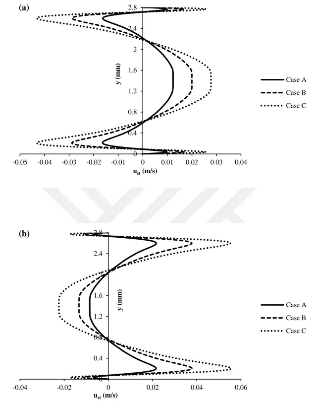
Figure 3.13 shows the time-averaged flow field in the enclosure for Case A-1 and Case A-3 at the end of the 40th acoustic cycle. The bottom wall of the enclosure is exposed to sinusoidal and half-sinusoidal temperature profiles for Case A-1 and Case A-3, respectively. Presence of the temperature gradients deforms the symmetric structure of the streaming observed in Case A. Expansion in the outer streaming vortices at the vicinity of the bottom wall and contraction in the outer cells near the top wall are observed in Case A-3 as the temperature of the bottom wall increases. Despite the deformation of the Rayleigh streaming structure in Case A-3 due to the temperature rise of the bottom wall, symmetry respect to the central vertical line is still observed. The symmetric nature of the flow is deformed completely in Case A-1. The lower outer streaming roll in the left portion of the resonator expands. Similar pattern is observed for the upper outer vortex in the right portion of the enclosure since the temperature of the top wall is higher in this section. The results demonstrate that the pattern of the flow in the enclosure depends strongly on the applied temperature profile to the bottom wall.

36

Figure 3.13: Streaming flow field in the enclosure at t=0.04s for (a) Case A-1 and (b) Case A-3.

Figure 3.14 depicts the distribution of the axial streaming velocity along the y-axis through the center of the streaming cells (x=L/4 and x=3L/4) for Case A, 1 and A-3 at t=0.04s. The axial streaming velocity is perfectly symmetric respect to the horizontal mid-line in both locations in Case A since the temperature of the bottom wall is kept at initial temperature such as top wall. The streaming velocity increases and reaches to its maximum value near the bottom wall in both Case A-1 and A-3 at x=L/4. The maximum positive streaming velocity is observed in Case A-1 since the sinusoidal temperature profile has the maximum wall local temperature at this point (x=L/4). Reduction in the streaming velocity is observed at the vicinity of the bottom wall in Case A-1 at x=3L/4 due to the lowest local temperature of bottom wall at this location. x (mm) y (m m ) 50 100 150 1 2 0.03 m/s

Frame 00106 Mar 2017PLOTF1

x (mm) y (m m ) 50 100 150 1 2 0.03m/s

Frame 00106 Mar 2017PLOTF1

(b) (a)

37

Figure 3.14: Variation of the x-component of the streaming velocity at t=0.04 s along the y-axis at (a) x=L/4 and (b) x=3L/4.

The time-averaged density profile along the vertical lines at x=L/4 and x=3L/4 for Case A, A-1 and A-3 at t=0.04 s is represented in Figure 3.15. Presence of temperature gradients leads to expansion in the streaming vortices, resulting in reduced density (Figure 3.15.a). As the density reduces, the streaming velocity enhances in the rarefied zones which can be observed in Figure 3.14.a in both Case A-1 and A-3. At x=3L/4, air is compressed near the bottom wall due to the low

0 0.4 0.8 1.2 1.6 2 2.4 2.8 -0.03 -0.02 -0.01 0 0.01 0.02 0.03 0.04 y ( m m ) ust(m/s) Case A Case A-1 Case A-3 0 0.4 0.8 1.2 1.6 2 2.4 2.8 -0.03 -0.02 -0.01 0 0.01 0.02 0.03 0.04 y ( m m ) ust(m/s) Case A Case A-1 Case A-3 (a) (b)

38

temperature of the wall at this section in Case A-1. As a result, the streaming velocity reduces in the dense zones. The density profile at both x=L/4 and x=3L/4 remain identical for Case A-3 due to the symmetric pattern of the half-sinusoidal temperature profile.

Figure 3.15: Cycle-averaged density profile along the enclosure height at t=0.04 s for Case A, A-1 and A-3 at (a) x=L/4 and (b) x=3L/4.

0 0.4 0.8 1.2 1.6 2 2.4 2.8 1.14 1.15 1.16 1.17 1.18 1.19 y ( m m ) ρ (kg/m3₎ Case A Case A-1 Case A-3 0 0.4 0.8 1.2 1.6 2 2.4 2.8 1.16 1.17 1.18 1.19 1.2 1.21 1.22 y ( m m ) ρ (kg/m3₎ Case A Case A-1 Case A-3 (a) (b)

39

Spatially non-uniform bottom wall temperature profiles induce axial and transverse temperature gradients in the enclosure. In order to investigate the transition behavior of the secondary flow due to the gradual enhancement in these gradients, additional cases are considered as listed in Table 3.3.

Table 3.3 : Cases with intermediate temperatures. Case Profile TBmax(K) Xmax (µm)

1-a Half Sinusoidal 300.5 60 1-b 301 1-c 302 1-d 304 1-e 306 1-f 308 2-a sinusoidal 300.5 2-b 301 2-c 302 2-d 304 2-e 306 2-f 308

The maximum displacement of the left wall is set to 60 µm and frequency of the left wall vibration is 1 kHz for all cases listed in Table 3.3. Figure 3.16 and 3.17 depict the cycle averaged flow field in the left portion of the enclosure at t=0.04 s for all cases mentioned here. The streaming velocities increase by the augmentation in the bottom wall temperature. In the half-sinusoidal heating cases (Figure 3.16), as the bottom wall temperature increases, the lower outer streaming vortex expands, and its center shifts towards the top wall and the core of the upper outer streaming roll moves towards the left wall. This is due to the spatial non-symmetry of the bottom wall temperature between 0 < x < L/2. The outer streaming roll at the bottom section expands in transverse direction and compresses the outer streaming roll at upper section in the sinusoidal heating cases (Figure 3.17). However the core of the upper streaming vortex remains at x=L/4.