İZMİR KATİP ÇELEBİ UNIVERSITY GRADUATE SCHOOL OF NATURAL AND APPLIED SCIENCES
A PRELIMINARY OFFSHORE WIND ENERGY POTENTIAL STUDY FOR BAY OF İZMİR: QUANTIFYING THE AIRFLOW DISTORTION ON LOCAL FERRYBOATS FOR ADJUSTMENT OF WIND DATA BY 3D CFD ANALYSES
M.Sc. THESIS Şahin GÜNGÖR
Department of Mechanical Engineering
Thesis Advisor: Asst. Prof. Dr. Ziya Haktan KARADENİZ
İZMİR KATİP ÇELEBİ UNIVERSITY GRADUATE SCHOOL OF NATURAL AND APPLIED SCIENCES
A PRELIMINARY OFFSHORE WIND ENERGY POTENTIAL STUDY FOR BAY OF İZMİR: QUANTIFYING THE AIRFLOW DISTORTION ON LOCAL FERRYBOATS FOR ADJUSTMENT OF WIND DATA BY 3D CFD ANALYSES
M.Sc. THESIS Şahin GÜNGÖR
(Y140105014)
Department of Mechanical Engineering
Thesis Advisor: Asst. Prof. Dr. Ziya Haktan KARADENİZ
İZMİR KATİP ÇELEBİ ÜNİVERSİTESİ FEN BİLİMLERİ ENSTİTÜSÜ
İZMİR KÖRFEZİ İÇİN RÜZGAR POTENSİYELİ BELİRLEME ÖN ÇALIŞMASI: 3 BOYUTLU HAD ANALİZİ İLE RÜZGAR VERİSİNİN DÜZELTİLMESİ İÇİN YEREL FERİBOTLAR ÜZERİNDEKİ AKIŞ BOZUNUMLARININ ÖLÇÜLMESİ
Yüksek Lisans Tezi Şahin GÜNGÖR
(Y140105014)
Makina Mühendisliği Bölümü
Tez Danışmanı : Yard. Doç. Dr. Ziya Haktan KARADENİZ
v
Şahin Güngör, a M.Sc. student of IKCU Graduate School of Natural and Applied Sciences student ID Y140105014, successfully defended the thesis entitled “A Preliminary Offshore Wind Energy Potential Study for Bay of Izmir: Quantifying the Airflow Distortion on Local Ferryboats for Adjustment of Wind Data by 3D CFD Analyses”, which he prepared after fulfilling the requirements specified in the associated legislations, before the jury whose signatures are below.
Thesis Advisor : Asst. Prof. Dr. Ziya Haktan KARADENİZ ... İzmir Katip Çelebi University
Jury Members : Prof. Dr. Gökdeniz NEŞER ... Dokuz Eylül University
Assoc. Prof. Dr. Alpaslan TURGUT ... Dokuz Eylül University
Date of Submission : 07 December 2016 Date of Defense : 04 January 2017
vii FOREWORD
We have been living in Izmir city which have a long sea shore and maritime is among our interests since childhood. I also work as a mechanical engineer in The Ministry of Transport, Maritime Affairs and Communication, therefore, my thesis supervisor and I decided to study about both maritime and wind energy assessment. I would like to thank advisor of my thesis Asst. Prof. Dr. Ziya Haktan KARADENİZ for his friendly assistance and important guidance. In this study, we tried some new engineering approaches thanks to him and during this period he helped and supported me whenever I need.
I am thankful to the İzmir Metropolitan Municipality, İzdeniz Inc. administrator and Özata Shipyard Company’s valuable engineers for providing me all needed data about the catamaran ship.
I would also like to express my deep gratitude to my parents. It would not have been possible for me to be here without their unfailing support and encouragement throughout my life.
January 2017 Şahin GÜNGÖR
ix TABLE OF CONTENTS Pages FOREWORD ... vii TABLE OF CONTENTS ... ix ABBREVIATIONS ... xi
LIST OF TABLES ... xiii
LIST OF FIGURES ... xv
SUMMARY ... xvii
ÖZET ... xix
1.INTRODUCTION ... 1
1.1 Ship Sourced Data for Meteorological Analyses ... 2
1.2 Wind Speed Bias Resulting from Ship Superstructure ... 5
1.3 Offshore Wind Energy Assessment by Using Ship Sourced Data .... 19
1.4 Can We Use the Local Ferryboats to Collect Wind Speed Data? ... 21
2.MATERIAL AND METHODS ... 25
2.1 Description of the Catamaran and Analysis Domain ... 25
2.2 Determination Of The Mesh Sizes And Quality ... 27
2.3 Determination Of The Boundary Conditions ... 28
3.RESULTS AND DISCUSSION ... 33
3.1 Wind Speed Bias Analysis for the Different Inlet Velocities ... 33
3.2 Wind Speed Bias Analysis for the Different Azimuthal Positions .... 43
4.CONCLUSION ... 59
REFERENCES ... 61
xi ABBREVIATIONS
SODAR : Sonic Detection and Ranging LIDAR : Light Detection and Ranging OWS : Observing Weather Ships VOS : Voluntary Observing Ships
WMO : World Meteorological Organization
ICOADS : International Comprehensive Ocean Atmosphere Data Set CFD : Computational Fluid Dynamics
CAD : Computer Aided Design
AIS : Automatic Identification System HAD : Hesaplamalı Akışkanlar Dinamiği NWP : Numerical Weather Prediction PIV : Particle Image Velocimetry
WAsP : Wind Atlas Analysis and Application Program MM5 : Mesoscale Meteorological Model
WASWind : Wave and Anemometer Based Surface Wind WAGES : Waves, Aerosol and Gas Exchange Study SST : Shear Stress Transport
xiii LIST OF TABLES
Page
Table 1.1 : New Beaufort Equivalent Scale ... 3
Table 1.2 : Measured Wind Speed Statistics ... 5
Table 2.1 : Statistics of the Mesh Size for Flow Domain ... 27
Table 3.1 : Wind Speed Bias for the Different Inlet Velocities ... 42
xv LIST OF FIGURES
Page
Figure 1.1 : Wind Speed Errors for Different Directions ... 6
Figure 1.2 : CFD Calculations for Bow-on Flow... 7
Figure 1.3 : 3D View of a Simple Tanker Model Airflow Distortion ... 7
Figure 1.4 : The Fractional Wind Speed Error for Tanker Used in CFD Study ... 8
Figure 1.5 : The Principal Shape of a Container Ship,Tanker and Bulk Carrier ... 9
Figure 1.6 : Comparison of the CFD and PIV Measurements ... 10
Figure 1.7 : The Flow Pattern around the Bridge of the Generic Models... 11
Figure 1.8 : Normalized Wind Speed Profile ... 11
Figure 1.9 : The CFD Model Results for a Flow over the Port Beam ... 12
Figure 1.10 : Dimensions of the Bluff Body Geometry ... 13
Figure 1.11 : Normalized Wind Speed Profiles at Different Distances ... 13
Figure 1.12 : The Normalized Wind Speed for Bow-on and Beam-on Flow ... 14
Figure 1.13 : Navy Ship Model ... 15
Figure 1.14 : The RRS. James Clark Ross Geometry ... 16
Figure 1.15 : Flow Contours for Bow-on and Beam-on Flow ... 17
Figure 1.16 : Wind Speed Bias and Vertical Displacement for Different Wind Directions ... 18
Figure 1.17 : Statistics for Wind Speed Observations ... 20
Figure 1.18 : Presentation of the Izmir Bay and Points of Trasnportation Piers ... 22
Figure 2.1 : Catamaran Ferryboat Figures Cruising in Izmir Bay ... 25
Figure 2.2 : SolidWorks Model of the Catamaran Ship. ... 25
Figure 2.3 : The Flow Domain Parts and Model Geometry ... 26
Figure 2.4 : Mesh Quality Presentations for the Flow Domain and Ship ... 24
Figure 2.5 : Atmospheric Boundary Layer Profile Presentation ... 28
Figure 2.6 : Wind Speed Vectors Used for the Inlet Determination ... 29
Figure 2.7 : Azimuthal Angle Presentation over the Flow Domain... 30
Figure 2.8 : Relationship of Relative Wind Speed and Azimuthal Positions ... 30
Figure 2.9 : Wind Speed Vector for the Different Azimuthal Positions ... 31
Figure 3.1 : Velocity Contour Presentation for the Different Inlet Velocities ... 35
Figure 3.2 : Dimensionless Free Strem Velocity in the Gap of the Catamaran ... 36
Figure 3.3 : Dimensionless Flow Contour for the Different Inlet Velocities ... 37
Figure 3.4 : Horizontal Dimensionless Flow Contour at the Anemometer Height. 39 Figure 3.5 : Streamlines around the Ship Geometry for Different Wind Speeds ... 40
Figure 3.6 : Volume Rendering Presentation at the Anemometer Site ... 41
Figure 3.7 : Wind Speed Bias Depending on the Wind Speeds ... 42
Figure 3.8 : CFD Result of a Previous Study for Bow-On Flow ... 43
Figure 3.9 : Velocity Contour for the Different Azimuthal Angles (0-135°) ... 45
xvi
Figure 3.11 : Dimensionless Velocity Contour Presentation for 0-135° ... 48
Figure 3.12 : Dimensionless Velocity Contour Presentation for 180-315° ... 49
Figure 3.13 : Horizontal Flow Contour at the Anemometer Height (0-135°) ... 51
Figure 3.14 : Horizontal Flow Contour at the Anemometer Height (180-315°) ... 52
Figure 3.15 : Streamlines around the Ship Model for Different Wind Directions .... 53
Figure 3.16 : Volume Rendering Presentation for Anemometer Site (0-135°) ... 55
Figure 3.17 : Volume Rendering Presentation for Anemometer Site (180-315°) ... 56
Figure 3.18 : Detail of the Anemometer Sites for the Catamaran and the Model ... 57
xvii
A PRELIMINARY OFFSHORE WIND ENERGY POTENTIAL STUDY FOR BAY OF İZMİR : QUANTIFYING THE AIRFLOW DISTORTION ON LOCAL FERRYBOATS FOR ADJUSTMENT OF WIND DATA BY 3D CFD ANALYSIS
SUMMARY
Humankind have an interest to obtain marine meteorological data for decades, therefore, constant and mobile meteorological stations have been used for the correct measurements. These meteorological data include wind speed and direction, sea surface and air temperature and cloud cover. Ship-mounted anemometers have been used for meteorological observations, obtaining the wind speed data and climate change analysis. Wind data are especially gathered and reported by Voluntary Observing Ships (VOS). World Meteorological Organization (WMO) created the VOS program to ensure reporting of the wind data from ships regularly. Ships participated this program are cargo or tanker ships which are in different shapes and sizes. Anemometers are usually sited on a mast above the bridge of ships where the effects of flow distortion may be severe. Therefore, determining the wind speed bias around anemometers is so important for the reliability of data. Despite the wide range of usage for gathering wind data, only a few studies have taken the air flow distortion into account caused by the ship’s structure. In those studies, cargo ships or tankers have generally been used for wind data distortion-modelling in computational fluid dynamics (CFD) analysis.
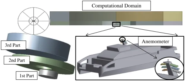
The aim of our study is quantifying the airflow distortion over local catamaran ships in Izmir Bay by 3D CFD analysis. 3D model of the catamaran ships is imported to Ansys CFX program and the air flow distortion caused by ship’s structure is analysed for different cases. The ship geometry has been modelled in detail to quantify the best results and the flow domain is made up of three bodies; one of them is a cylindrical core where the ship geometry is also in the centre of this layer. This layer’s radius is 1 ship lengths and height is 2 ship heights. This layer was arranged with detailed mesh sizes which were minimum 0.005 H, where the H was the height of the bridge above the waterline. Second part of flow domain is a ring shaped layer whose radius is 5 ship lengths and height is 2 ship heights. First part of the domain is in the centre of the second domain and they together form a disk like structure. Last part is also a cylindrical part which stands above the first and second parts. Third part’s radius is 5 ship lengths and height is 28.4 meters. These three flow domains form a model which has a radius of 5 ship lengths and a height of approximately 5 ship heights. Different mesh sizes were studied to quantify the air flow distortion in the flow domain correctly. The mesh sizes have been decreased at the positions closer the ship hull and increased away from the ship hull where the flow didn’t vary a great deal. Other air flow distortion studies in the literature used rectangular prism domains. In this study, the flow domain is sliced 8 equal parts. The cylindrical domain has advantages for correct results because the mesh model is fixed for every
xviii
analysis and wind directions can be changed simply with cylindrical domain’s 45° pieces.
When the wind is impacted directly from the ship's bow, wind speed biases are approximately 5% around the anemometer site. Free stream velocity is accelerated up to 10% for 45° clockwise air flow that is similar with 315° wind direction. Accelerated flow regions are close to the anemometer position. The most important reason of the accelerated flow regions is the negatively inclined surface which is positioned in front of the master cabin of the ship. When the wind is impacted directly from beam (90° and 270°) of the catamaran, wind speed biases are between 17-20%. For the case that the air flow is affected from 135° and 225° clockwise, the flow accelerated between 6-8% . Decelerated flow regions are intensely behind the ship’s mast structure. When the wind is directly impacted from astern of the ship (180°), the mast behaves as an obstacle behind the anemometer. Because of this reason, the average wind speed values are approximately 30% lower than 𝑈10.8. Catamaran ship model has a closed part at the ship’s bow because of the platform which using for embarking and disembarking of the passengers. If the catamaran ship model was drawn symmetrically, the wind speed bias pairs for 45 and 315°, 90 and 270 °, 135 and 225° would be same. CFD analysis outputs were compared with information in the literature by means of wind data bias around the ships. Results of this study can be used for correcting the data collected from ship’s anemometer and to obtain the accurate offshore wind data to determine the offshore wind energy potential in Izmir Bay.
xix
İZMİR KÖRFEZİ İÇİN RÜZGAR ENERJİSİ POTANSİYELİ BELİRLEME ÖN ÇALIŞMASI: 3 BOYUTLU HAD ANALİZİ İLE RÜZGAR VERİSİNİN
DÜZELTİLMESİ İÇİN YEREL FERİBOTLAR ÜZERİNDEKİ AKIŞ BOZUNUMLARININ ÖLÇÜLMESİ
ÖZET
Sürdürülebilir üretim sağlayan su üstü rüzgar enerjisi, çevre dostu teknolojisiyle gün geçtikçe önem kazanan yenilenebilir enerji kaynağıdır. Su üstü rüzgar enerji üretimine yönelik çalışmalar Dünyanın denize kıyısı olan birçok gelişmiş ülkesinde hükümet programlarına dâhil edilmiştir. Bunun başlıca nedenleri; deniz ve okyanus bölgelerinde daha kararlı ve yüksek rüzgar potansiyelinin bulunması, çevreye etkilerinin karasal rüzgar türbinlerine göre çok daha az olmasıdır. Bunun yanında montaj ile işletme ve bakım maliyetlerinin yüksekliği de hâlâ karasal türbinlerinin daha sık kullanılmasının nedenlerindendir. Su üstü rüzgar potansiyelinin belirlenmesinde meteoroloji gözlem direkleri, uydu destekli donanımlar ve ses-ışık yoluyla tarama yapan cihazlar kullanılmaktadır. En klasik yöntem olan gözlem kuleleri uzun ölçüm periyotları sonucunda (en az 1 yıllık ölçüm) rüzgar potansiyeli belirlemek için kullanılır. Ses veya ışık yollu tarama cihazlarının kullanımı ise rüzgar potansiyelinin belirlenmesi için çok maliyetli yöntemlerdir. Uydu destekli donanımlar yardımıyla oluşturulan, geniş alanlarda potansiyel belirlemeye yarayan ve kullanımı gitgide yaygınlaşan rüzgar haritalarında çözünürlük çok düşüktür ve verilerin doğrulanması gerekir.
Okyanus ve deniz üstü meteorolojik verilerin elde edilmesi çalışmaları on yıllardır insanoğlunun uğraş alanıdır. Bu meteorolojik verilerin doğru elde edilmesi için gerek sabit gerekse de hareketli meteorolojik ölçüm istasyonları kullanılmıştır. Su üstü alanların genişliği nedeniyle sabit meteorolojik istasyonlar ölçümlerin sağlıklı şekilde yapılmasında yetersiz kalmış ve özellikle ticari gemiler yardımıyla bu verilerin elde edilmesi, toplanması fikri ortaya çıkmıştır. Gemiler yardımıyla meteorolojik verilerin elde edilmesi amacıyla Okyanus Meteoroloji Gemileri (OWS) adı verilen ve donanımlı ölçüm cihazlarına sahip gemiler oluşturulmuştur. Ancak, bu gemilerin sayılarının az olması ve okyanus üstü ölçüm yapılacak alanların genişliği nedeniyle, sefer yapan ticari gemilerin (tanker, kargo, yük gemileri vb.) veri toplamada kullanılması için Dünya Meteoroloji Örgütü (WMO) tarafından Gönüllü Gözlem Gemileri (VOS) programı oluşturulmuştur. Bu program ile programa dâhil olan on binlerce ticari gemiden elde edilen meteorolojik ölçüm verileri Uluslararası Kapsamlı Okyanus Veri Seti (ICOADS) tarafından toplanmış ve arşivlenmiştir. Arşivlenen bu veriler; rüzgar hızı ve yönü, su yüzeyi sıcaklığı, hava sıcaklığı ve bulutluluk oranı verilerini içerir. Bu ölçümler arasında en önemli meteorolojik veri ise rüzgar hızı ve yönü bilgisidir. Bilindiği üzere su üstü seyir koşulları rüzgar hızı ve yönü ile dalga yüksekliğine bağlı olarak belirlenmektedir. Bu önemi nedeniyle, gerek ölçüm yapılan verilerin doğruluğu, gerekse de ölçüm yapan gemilerin inşai yapıları nedeniyle meydana gelen ölçüm sapmalarının tespit edilmesine yönelik olarak birçok
xx
çalışma yapılmıştır. Literatürdeki ilk rüzgar çalışmaları Bofor Göstergesi belirleme üzerine yapılan çalışmalar olup, genellikle yerel bölgelerdeki ölçüm verileriyle gösterge oluşturulmuştur. Bofor Göstergesi bölgesel olarak ölçümü yapılan rüzgar verilerindeki, en az ve en çok rüzgar şiddetinin 0-12 arasındaki ölçekle gösterilme şeklidir. Skala belirleme üzerine yapılan matematiksel yaklaşımların en önemlisi ve hâlâ kabul göreni ise Lindau tarafından yapılan çalışmadır. Bofor Göstergesi, rüzgar hızını ölçebilen mekanik anemometrelerin geliştirilmesiyle birlikte önemini yitirse de hava tahminciler ve denizciler tarafından hâlâ kullanılmaktadır.
Gemi anemometreleriyle yapılan rüzgar ölçümlerinde geminin kendi yapısından kaynaklanan akış bozunumlarının belirlenmesi, verinin doğruluğu açısından son derece önemlidir. Anemometre bölgesine gelen rüzgar hızında geminin inşai yapısı nedeniyle ivmelenmeler ve zayıflamalar olmaktadır. Literatürde geminin kendi yapısından kaynaklı akış bozunumlarına dair çalışmalar hem rüzgar tüneli hem de hesaplamalı akışkanlar dinamiği (HAD) analizleriyle ortaya konmuş olup, hata miktarları gemi şekil ve büyüklüğüne bağlı olarak hesaplanmıştır. Taylor, CSS Dawson isimli gemi üzerinde akışı inceleyerek, rüzgar hızındaki ivmelenme ve yavaşlama bölgelerini ve hata miktarlarını HAD analizi ile belirledi. Ayrıca, rüzgar tüneli çalışması ile 90° ‘lik açılarla gelen rüzgarın etkisiyle, anemometre bölgesinde meydana gelen hata miktarını da grafikledi. Thomas ise Lindau tarafından oluşturulan Bofor Göstergesini geliştirerek, deniz seviyesinden 10 m yükseklikteki rüzgar hızındaki hatayı düzelten 3. dereceden bir polinom denklemi türetti. Fakat bu denklem geminin şekil ve büyüklüğünden bağımsız olarak sadece matematiksel bir yaklaşım olduğu için sağlıklı sonuçlar vermemektedir. Literatürdeki ilk kapsamlı HAD modeli RRS Charles Darwin gemisi üzerindeki akışın analizlerinde oluşturulmuştur. Bu çalışmada anemometre bölgesindeki hata miktarları, hem gemi burnundan hem de geminin iskelesinden gelen akış için analiz edilmiş ve hesaplanmıştır. Bu çalışma sonrasında hesapların genellenmesi ve tüm tanker ve konteynır gemilerine uyarlanabilmesi adına, x/H ve z/H boyutsuz değerler için rüzgar hızı hataları hesaplanmıştır. Bu çalışmalarda, “x” köprü üstündeki yatay konum, “z” düşey konum, “H” ise deniz suyu seviyesinden köprü üstüne kadar olan düşey mesafedir. Moat ve Yelland ise RRS James Clark Ross isimli araştırma gemisi üzerinde detaylı bir HAD analizi yapmıştır. Bu çalışma analizlerinde atmosferik sınır tabaka koşulları göz önüne alınmış olup, geminin burnunda bulundan anemometrenin iskele ve sancağından 0°, 10°, 20°, 30°, 50°, 70°, 90° ve 110° ‘lik açılar için rüzgar hızı hataları hesaplanmıştır. Literatürdeki en kapsamlı çalışma olan bu çalışma ile farklı yönlerden etkiyen rüzgarın anemometre bölgesindeki etkisinin önemi kanıtlanmıştır.
Bu çalışmada, İzmir Körfezinde yolcu taşımacılığı yapan katamaran tipteki feribotlar modellenerek, gemi üzerindeki hava akış bozunumlarının ve anemometre bölgesindeki rüzgar hızı hatalarının rüzgar hızı ve rüzgar yönlerindeki değişimlere bağlı olarak analizi ve hesaplanması amaçlanmıştır. Özata Tersanesinde inşa edilen 39 m tam boy uzunluk, 11,6 m genişlikteki 426 yolcu kapasiteli katamaran gemiler SolidWorks bilgisayar destekli çizim programı yardımıyla bire bir ölçekle modellenmiştir. Bu model Ansys CFX analiz programına transfer edilerek, 3 katmandan oluşan silindirik bir akış hacminin tabanında, bu hacmin merkezine yerleştirilmiştir. Akış hacminin birinci katmanı merkezinde geminin bulunduğu çekirdek katman olup, hacmin yarıçapı geminin uzunluğunun 2 katı ve yüksekliği gemi yüksekliğinin 2 katı uzunluktadır. Bu katman, geminin bulunması nedeniyle
xxi
akış hacmindeki en önemli katman olup, üçgen yapıda ve çok küçük boyutlarda ağ yapısı ile örülmüştür. Silindirik akış hacmindeki ikinci katman, birinci katmanı saran bir yüzük şeklindedir ve yarıçapı 5 gemi uzunluğunda, yüksekliği ise 2 gemi yüksekliğindedir. Son katman ilk iki katmanın üzerinde bulunan ve yarıçapı 5 gemi uzunluğu, yüksekliği yaklaşık 3 gemi yüksekliğinde (28,4 m) olan, akışın önemli olduğu bölgelerden uzak olması nedeniyle daha büyük ağ yapısı ile örülen silindirik yapıdır. Akış hacmi toplamda 5 gemi uzunluğu yarıçapında ve yaklaşık 5 gemi yüksekliği uzunluktadır. Akış hacminde gemiye yakın bölgeler için ufak ağ yapısı ve gemiden uzaklaştıkça büyüyen ağ yapısıyla örülmüş olup, toplam ağ sayısı yaklaşık 15𝑥106 ‘dır. Analizler 25°C ‘ deki hava koşulları için yapılmış olup, analiz giriş kısmında rüzgar hızları atmosferik sınır tabaka koşulları dikkate alınarak tanımlanmıştır. Analizlerde kayma gerilmesi taşınımı (SST model) türbülans modeli seçilerek akışın en iyi ve detaylı çözülmesi hedeflenmiştir. İzmir Körfezinde seyir yapan katamaranların ortalama seyir hızları gemilerin üzerinde bulunan otomatik tanımlama sistemi (AIS) cihazları ile tespit edilerek, analizlerde gemi hareketli olacak şekilde seyir hızı 6 m/s olarak tanımlanmıştır. Analizlerde kullanılan akış hacmi 8 eşit parçaya bölünerek, 10 m/s serbest rüzgar hızında 45° ‘lik açılarla gelen farklı rüzgar yönleri için, ağ yapısı sabit tutularak sadece giriş parçalarının açıya göre tanımlanması yoluyla analizlerde kolaylık sağlanmıştır. Ayrıca bu çalışmada, farklı serbest rüzgar hızları için gemi burnundan gelen akışta meydana gelen bozunumlar da analiz edilmiştir. Bu analizlerde 0, 5, 10, 15, 20 m/s serbest rüzgar hızları atmosferik sınır tabaka koşulları da dikkate alınarak analizler yapılmıştır. Literatürde ise, gemi yapısının farklı rüzgar hızlarında akışa etkisi ile ilgili olarak çok sınırlı çalışma bulunmakta olup, çalışma sonuçları ve literatürdeki sonuçlar uyum göstermektedir.
Bu çalışmada, 6 m/s ortalama feribot hızı ve 10 m/s serbest rüzgar hızı için rüzgarın gemiye göre 45° ‘lik aralıklarla etkimesi durumundaki akış bozunumları ve rüzgar hızı hataları analizleri yapılmıştır. Analiz sonuçları ile akış hacmi içerisinde ve gemi üzerinde akışın ivmelendiği ve zayıfladığı bölgeler belirlenmiş olup, rüzgar hızı hataları da hesaplanmıştır. Rüzgar gemi burnundan etkidiği anda (0-360°) anemometre bölgesindeki hata yaklaşık olarak % 5’ tir. Rüzgar gemiye göre saat yönünde 45° ve 315° lik açılarla geldiğinde, akış yaklaşık olarak % 10 ivmelenmiştir. Rüzgar geminin iskele ve sancağından etkidiğinde (90° ve 270°) hata payları % 17-20 civarındadır. Rüzgar gemiye saat yönünde 135° ve 225° açıyla geldiğinde ise, akış hızı % 6-8 civarında ivmelenmiştir. Geminin yatay eksenine (x ekseni) göre aynalanmış açıların hata değerleri birbirine çok yakındır. Bunun nedeni geminin burun kısmında bulunan, yolcu indirme-bindirme platformu ve motorunun bulunduğu kısım hariç geminin simetrik olmasıdır. Rüzgar geminin kıç tarafından etkidiğinde (180°) ise, akış anemometre bölgesinde yaklaşık olarak % 30 zayıflamıştır. Bunun nedeni gemi direğinin anemometre bölgesi öncesinde duvar etkisi yaratmasıdır. Çalışmalarımızda 6 m/s ortalama feribot seyir hızı ve farklı rüzgar hızları için yapılan HAD analizleri ise büyük benzerlikler göstermiştir. Bu analizler rüzgarın geminin burnundan geldiği durum için yapılmış olup, sonuçların hepsinde anemometre bölgesinde ivmelenme görülmüştür. Bunun nedeni gemiye göre karşıdan gelen rüzgarın, kaptan köşkü önünde bulunan eğik yüzey sayesinde hızlanmasıdır. Farklı hızlarda akışın incelendiği analiz sonuçlarında, geminin baş ve kıç güvertesi ile gemi direğinin arka bölgesinde akış zayıflamaları görülmüştür. Akış zayıflamalarının nedeni, gemi yapısından kaynaklı olarak bu kısımlardaki durdurma etkisidir. Ayrıca, sonuçlar serbest rüzgar hızı arttıkça rüzgar hızı hatalarının
xxii
azaldığını ortaya koymuştur. Sonuçlar grafiklenerek, hata - rüzgar hızı ve hata – rüzgar yönü ilişkileri formülize edilmiştir.
Bu çalışmanın analiz sonuçları sayesinde, İzmir Körfezinde seyir yapan gemiler kullanılarak körfez içi su üstü rüzgar enerjisi potansiyeli doğru olarak belirlenebilecektir. Gemilerden toplanacak rüzgar verileri rüzgar hızı ve yönüne bağlı olarak düzeltilerek, ek donanımlar ve maliyetler gerekmeden yıl boyunca İzmir Körfezindeki su üstü rüzgar hızlarına ulaşılabilecektir. Bu çalışma su üstü rüzgar enerji potansiyeli belirleme adına temel bir çalışma olup, aynı çalışma sistematiği içinde farklı gemi tipleri için analizler yapılarak, farklı bölgelerdeki potansiyel belirleme çalışmalarında da kullanılabilir. Ayrıca bu çalışmanın analiz sonuçları, meteorolojik araştırma veya gözlem gemilerine ihtiyaç duyulmadan rüzgar verisi toplanmasına olanak sağlamaktadır.
1 1. INTRODUCTION
Offshore wind is a renewable energy source which ensures an eco-friendly technology to produce sustainable energy. Because it has higher wind potential than onshore, lower effects of surrounding on wind flow etc., the countries all over the World have assimilated offshore wind energy into their government’s energy planning. Meteorological observation towers, satellite based instruments, sonic and light detection and ranging devices (SODAR and LIDAR) can be used for determination of the offshore wind resources. Usage of the meteorological mast or well-equipped towers are the original method to estimate the wind energy resource, but it requires more time (minimum 1 year) than the other methods. SODAR and LIDAR methods are too costly for determination of the offshore wind energy potential. Investigators studying on this field are mostly using satellite based measurements. Thanks to feasibility studies, satellites can predict higher wind power resources but wind energy maps’ resolutions are very low.
Ships are cruising continuously on the sea and collecting wind data for a safe operation. This data can also be used for meteorological purposes including offshore wind energy potential determination. Predicting the wind energy potential more accurately by validation of the satellite data and to propose better models for wind energy potential studies. Therefore, ship mounted anemometers can help for correction of the measurements obtained from different type of wind power resources.
Ships have been used to gather marine meteorological data for years. These meteorological data include wind speed and direction, air and sea surface temperature and cloud cover. Although all ships have devices to gather some meteorological data, World Meteorological Organization (WMO) has created the Voluntary Observing Ships (VOS) program to report meteorological parameters at marine surface regularly. Ships which have participated VOS program are mostly
2
merchant ships employed in the ocean. International Comprehensive Ocean Atmosphere Data Set (ICOADS) have collected and archived these measured meteorological observations through VOS program. Studies about wind speed adjustment and air flow distortion were used these data set to quantify wind speed bias. Wind speed reports from VOS are obtained from anemometers which are permanently mounted over the bridge or on a mast of the ship’s bow, to give an indication of the wind conditions. Despite the wide range of usage of ships for gathering wind data, a few studies have taken the air flow distortion caused by the ship’s structure into account. Because, there have been two critical problems to evaluate the accurate wind speed; shape (type) and size of merchant ships and anemometer location on ships.
1.1 Ship Sourced Data for Meteorological Analyses
Wind speed adjustment studies in the literature consist of mathematical - statistical approaches, wind tunnel calculations and CFD analyses. Early mathematical-statistical studies were for the determination of Beaufort Scale in local regions. The Beaufort scale, which is used in marine forecasts, is an empirical measure for describing wind intensity based on observed sea conditions (MetOffice, 2016). It is a system of estimating and reporting wind speed; therefore, evaluation of this scale varies human to human. In order to standardization and generalization of forecasting and estimation of the wind speed, people who are interested in meteorological observations’ data have studied about this scale.
Lindau (1995) compared the six North Atlantic Ocean weather stations’ wind speed data with measured wind speed data from merchant ships and developed a Beaufort Equivalent Scale. New Beaufort Scale was calculated with average values of VOS and Ocean Weather Ships (OWS) individual reports. These averages fulfil two conditions: their mean accuracy was equal and they contained the same natural variability. Wind observations from OWS in the North Atlantic showed that OWS measurements are much more accurate than VOS estimates. The difference in accuracy could be quantified. The new Beaufort equivalent scale (given below) was valid for a height of 25 m above the sea level.
3
Table 1.1 : New Beaufort Equivalent Scale, Valid for a Height of 25 m above Sea Level (Lindau, 1995).
Bft 0 1 2 3 4 5 6 7 8 9 10 11 12
Knots 0 2.3 5.4 9.5 15.0 20.5 25.5 30.9 36.8 43.2 50.6 58.9 68.8
Lindau’s Beaufort Scale was valid only in North Atlantic; therefore, for other regions it should be converted to different scales. Proposed method was important, because, constant meteorological stations’ and merchant ships’ data were used together but, it wasn’t enough for generalizations.
Thomas et al. (2005) focused on methods to homogenize wind speed measurements from ships and buoys. The observations are performed either visually or by ship mounted instruments. Wind data from weather buoys moored in Canadian waters of the northeast Pacific and northwest Atlantic, and data from ships passing near these buoys were used in this study. This study aimed to quantify and remove the residual inhomogeneity (Yelland et al., 1997;2002) of unknown source and develop methodology to adjust measured wind data from different sources. The Canadian Marine Environmental Data Service (MEDS) provided data from three offshore buoys in the northeast Pacific and six in the northwest Atlantic. VOS reports came from ICOADS, obtained from ship log books. Anemometer heights varied between 10 to 40 m heights. Data of wind speed distributions for east and west coasts’ observations for measured winds are analysed statistically, and reported wind speed values (𝑈𝑧) are corrected (𝑈10𝑁) to include the atmospheric boundary layer effect by
using following equation (Eq. 1.1);
𝑈10𝑁 = 𝑈𝑧× ln( 10 0.0016) ln (0.0016)𝑧 = 𝑈𝑧 × 8.7403 ln(0.0016)𝑧 (1.1) The most important source of inhomogeneity between the anemometer-derived ship wind speeds and buoy results is different measurement heights. Thomas applied a conversion to estimated wind speed by improving the method offered by Lindau and developed a third-order polynomial which homogenizes the wind speed quite closely. This study applied the conversion from estimated wind speed 𝑈𝐸 to Lindau-adjusted wind speed 𝑈𝐸𝐿 using this polynomial;
4
This study showed that adjusting measured wind speeds to height of 10 m (atmospheric reference height) significantly improves the agreement between ship and buoy wind speed values measured at between 20 and 40 m.
Kent at al. (2005) studied about quantifying the meteorological measurement errors by using Voluntary Observing Ships’ wind speed, surface pressure, air temperature, humidity and sea-surface temperature measurements and observations obtained for the period between 1970 to 2002. They used the semivariogram method to estimate the random errors by attempring to separate the spatial and random components in variability (Kent, et al., 2005).
Wind data set obtained from VOS adjusted for height and Beaufort scale. There was little difference between random error estimates calculated separately for visually estimated and anemometer-measured wind speeds. This study was a general numerical based study and it was not enough to quantify the wind speed bias, because there were no VOS shape-size modelling and anemometer’s measurements could include calibration errors.
Thomas et al. (2008) also examined effect of anemometer height for wind speed adjustment. In this study, measured and estimated wind speed data obtained from ICOADS was used to show alteration of wind speed values for years. They used a method that could be employed to account for remaining inhomogeneties and thereby improve the quality of the marine wind climate record. The adjustment that was proposed by Lindau was modified by Thomas et al. (Thomas, et al., 2005) and a new third-order polynomial (Eq. 1.2) formula was offered for determining wind speed adjustment. Anemometer heights increased in early 1980s, and observed wind speed values increased during the same period. This study showed that annual average of the estimated wind speed became greater than the measured after 1982.
Bruce Ingleby (2010) studied about different type of ships and buoys wind speed measurements and factors affecting these data quality. Wind speed measurements obtained from ships and buoys for 2007 and 2008 have been compared with values from the operational Met Office global numerical weather prediction (NWP) system.
5
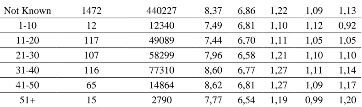
Table 1.2 : Measured ship wind speed statistics for 2007 by anemometer height, (Ingleby, 2010).
Anht (m) No. of Stations No. of Reports Mn O Mn B Ratio RatioA Adj
Not Known 1472 440227 8,37 6,86 1,22 1,09 1,13 1-10 12 12340 7,49 6,81 1,10 1,12 0,92 11-20 117 49089 7,44 6,70 1,11 1,05 1,05 21-30 107 58299 7,96 6,58 1,21 1,10 1,10 31-40 116 77310 8,60 6,77 1,27 1,11 1,14 41-50 65 14864 8,62 6,81 1,27 1,09 1,17 51+ 15 2790 7,77 6,54 1,19 0,99 1,20
In Table 1.2, “Adj” is mean speed at a height using Eq. 1.1 and “RatioA” is the ratio after the reported wind speeds have been adjusted to 10 m. This wind speed adjustment process was made with a logarithmic equation (Eq. 1.2). Wind speed data should be divided by this value to find the estimated wind speed at 10 m. This table also shows that wind speed measurements are generally stronger for higher anemometers. In this study, measured and estimated wind speed data was given depending on vessel types. A default anemometer height was estimated for each vessel type and used if the vessel type is known but the anemometer height is not. The highest anemometers were on the passenger ships followed by liquid tankers, container ships, bulk carriers and the lowest were on the research vessels, coast guards and trawlers. The results showed that ship based measurements of sea surface wind speed display upward trend due to increases in anemometer height. Wind data obtained from passenger ships, ferries, refrigerated ships and yachts appeared higher both before and after adjustment.
1.2 Determination of the Wind Speed Bias Resulting from Ship Superstructure
Visually estimated or measured wind speed data obtained from the merchant ships was used for mathematical and statistical studies. But, effects of ship superstructure on the airflow distribution and anemometer location over the ships are also important for the meteorological observations. Investigations about the airflow distortion around the anemometer sites on VOS models have been carried out experimentally using wind tunnel and numerically using commercial CFD codes. Different type of VOS and meteorological research ships were modelled to understand the acceleration
6
and deceleration regions of the airflow. They generally used rectangular prism models (a bluff body that is a very small model of the ship) to quantify the wind speed bias in wind tunnel studies and a computational domain was set to calculate the airflow distortion around the anemometer sites in CFD studies. Both approaches proved that wind speed data obtained from VOS’ estimates and observations definitely contain bias at different rates.
Taylor et al. (1997) used a model of small research ship, CSS Dawson, for a wind tunnel study and focused on the fact that, anemometer measurements on ships include some bias. Research ships have an anemometer that is mostly mounted over the wheelhouse and the wind flow around the anemometer can be disturbed because of the structure of the ship. Using CFD and wind tunnel methods, this is the first comprehensive air flow distortion study in the literature.
Figure 1.1 : Wind Speed Errors for Different Directions Measured In Wind Tunnel Study (Taylor, et al., 1997).
Taylor et al. also determined accelerated and decelerated air flow regions around the anemometer on the ship experimentally by a wind tunnel study (Fig 1.1). The wind flow effects depend on the direction was examined and wind speed biases were determined for 90° directions all around the ship. Around the anemometer sites the airflow was generally varied by -10 to 10 percent. When the wind flow is directly from the bow, the flow decelerated below sites of the accommodation block and accelerated over the accommodation block (Fig. 1.2). For research ships, when wind from either beam the wind speed value was overestimated and for wind from astern, the anemometer was in the wake of the accommodation block.
7
Figure 1.2 : CFD Calculations for Bow-on Flow over the CSS Dawson. The Numbers Indicate the Percentage Error In Each Region (Taylor, et al., 1997).
Taylor evaluated winds speed reports depended on the different anemometer heights. The fraction of anemometer measurements has increased with time as has the average height of the anemometer. Three different sized oil tankers were modelled as a rectangular block and air flow distortion was determined over the model. First tanker model was modelled with detailed mesh and the others modelled with coarser mesh for computational efficiency.
Figure 1.3 : 3D View of a Simple Tanker Model and Detailed View Showing Airflow Distortion over the Stern Section (Taylor, et al., 1997).
Bridge to deck height (D) was an important scaling factor for comparing the results of tanker models. CFD results showed that Tanker 2 and Tanker 3 had a similar
8
pattern of wind speed error for heights of less than around 8 m, but the magnitude of the decelerations differed by up to 20 percent in profiles obtained near the front edge of the bridge.
Figure 1.4 : (Left) Dimensions for the Tanker Models Used In the CFD Studies. (Right) The Fractional Wind Speed Error for Each of the Three Tanker Models at a Distance (x) from the Wheelhouse Where x/D= 0.6 (Taylor, et al., 1997).
All three models showed that at a height above the wheelhouse at any position having values greater than 0.5D any anemometer sites would give an overestimate of the wind speed of up to 5 percent. The fine meshed model’s (Tanker 1) CFD results showed that at a height of about 4 m above the bridge, the maximum acceleration was around 13 percent and the large deceleration below this height. This study showed that wind data obtained from ships are affected by the air flow distortion around the ship. Similar with this study’s results (Fig. 1.4), there is a shear layer that separates the accelerated and decelerated flow regions for all different inlet velocities and directions in our study.
A PhD thesis Moat (2003) and a series of papers were published by Moat et al. (2004, 2005, 2006 and 2015) with a deeper investigation on the topic. They focused on 3D cargo ship, container or tanker/bulk carrier models, which are represented by simple rectangular prisms, to determine the air flow distortion around ship’s anemometers caused by ship’s superstructure. It is mentioned that there were so many kinds of merchant ship which have different sizes and it would be impractical
9
to study about each individual ship. So, a method to describe the shapes of VOS and container ships was presented. Container and tanker/bulk carrier models were generally used in air flow distortion studies, because the most of the VOS that reports the wind speed measurements were this type of merchant ship. Merchant ships were basically modelled as seen in Fig. 1.5 with generalized dimensions representing the ship geometry as; the bridge to waterline height (BH), the length of overall (LOA), the breadth of the ship (B) and the length of the ship’s bridge (L).
Figure 1.5 : a) Represents The Shape and Principal Dimensions of Block Geometry of a Container Ship and (b) Represents of a Tanker/Bulk Carrier (Moat, et al., 2005).
Moat (2003) studied about airflow distortion around the anemometer sites and in this study wind tunnel and CFD analysis were used for examining the flow distributions. The generic tanker, container ship and deck house block geometries were scaled by approximately 1/50 to create the largest model possible without causing undue blockage of the flow. The Reynolds number of the wind tunnel experiment was in the same Reynolds number regime as the full-scale flow, so the model and the full-scale flow would have dynamically similar results. A series of flow visualization tests (smoke injection) above the bridge of the tanker and container ship were performed for determining the structure of the flow above the bridge of the ships. The smoke tests were performed at 5 m/s using a smoke wand to examine the flow along the centreline of the ship. A flow characterization study with Particle Image Velocimetry (PIV) measurements was also reported to measure the velocity field above the bridge of the merchant ship models. Three wind tunnel experiments were examined by comparing wind speed profiles to determine the accuracy of wind speed data and simple equations were derived to define the flow pattern and the magnitude of the wind speed above the ship models. Wind tunnel experiments’ data was obtained only for some flow cases to compare CFD and in situ data. In general, usage of wind
10
tunnels could be costly and the studies were limited by the wind tunnel speed and the physical size of the model.
Figure 1.6 : a) The CFD predicted wind speed maximum from each of the three
scale geometries compared with PIV measurements, b) The CFD simulation of the flow over a cube of height H=0.2 m in a boundary layer wind tunnel. The figure shows the velocity field normalised by the upstream wind speed, at height H, of 5.4 ms-1, (Moat, 2003).
Wind tunnel experimentation is time consuming and although producing high quality data, the PIV system has optical and technical limitations. For this reason, usage of CFD is as an alternative method to simulate the air flow over ships (Moat, 2003). VECTIS CFD software code was used for airflow distortion analysis in the computational domain. CFD experiments were examined for two scenarios; when the ships were modelled into one to one scale and modelled as wind tunnel studies’ sizes. Atmospheric boundary layer profile was taken into account for the flow determination. The bias in the PIV measurements was investigated by performing CFD models of the actual wind tunnel geometry. The CFD investigation for the airflow in the wind tunnel showed that the wind speed at the measurement location was accelerated by up to 9% by the downstream wind tunnel contraction. Applying this correction the magnitude PIV measurements agreed to within 10% of the CFD measurements. In situ data has a great agreement with CFD measurements and it confirmed the CFD results, but PIV measurements overestimated approximately 20% when compared with in situ data (Fig. 1.6). CFD model results were determined both qualitatively and quantitatively for validation of the air flow distortion and this study proved that if the anemometer positions on the ship are known, the wind speed measurement above the bridge can be corrected for the effects of airflow distortion.
11
Moat et al. (2005) used CFD code to model the flow over 3D VOS shapes described Fig 1.5. This commercial CFD code was previously used to study the air flow distortion over ships.
Figure 1.7 : The General Flow Pattern around the Bridge of a Generic Container and Tanker/Bulk Carrier, (Moat, et al., 2005).
Figure 1.7 shows the accelerated and decelerated flow pattern over generic container and the tanker/bulk carrier model. Close to the top of the bridge the airflow is decelerated and a standing vortex is produced in front of the bridge and there is flow separation at the upwind edge of the bridge. Above the decelerated region there is a shear layer where the wind speed is equal the free stream value and above the shear layer, the wind speed is accelerated.
Figure 1.8 : Normalized Wind Speed Profile above Tanker/Bulk Carrier at a Distance of x/H=0.5 Back From the Edge of The Bridge (x/H=0=z/H), (Moat, et al., 2005).
In Figure 1.8, “H” is the bridge to deck height, “z” is the vertical axis from the beginning of the bridge and “x” is the horizontal axis from the bridge. These axes
12
were presented in Figure 1.7. The profile was normalized by the free stream or undistorted flow, obtained from the CFD simulation by Moat et al. (2004). It was a general study about air flow distortion over the tanker and container ships, the anemometer locations of VOS weren’t available. So, it was not possible to correct VOS’ wind speed observations directly with the results of air flow distortion. Results showed that anemometer location on merchant ships may suffer wind speed biases of between -100% and +11%.
More realistic studies were presented by Moat et al. (2006) which are about air flow distortion caused by the ship’s structure and 3D CFD model was used. In this two-part study, firstly the flow around a 3D bluff body was modelled by VECTIS CFD code to quantify the airflow distortion. After validating the CFD code, the flow around the selected ship geometry was placed in the centre of a flow domain with an overall length of 9 ship lengths and a height of 2 ship lengths.
Figure 1.9 : The CFD Model Results for a Flow over the Port Beam of the RRS Charles Darwin. The Arrows Represent the Velocity of the Flow at Each Computational Cell, and the Variable Mesh Density Can Be Seen.
The inlet of the computational flow domain was defined with a wind speed profile that varied logarithmically with height, z. Different cases were calculated for 5, 10 and 15 m/s wind speeds. Up to 6 𝑥 105 computational cells were used to simulate the flow distrubition. The minimum cell size in the model was 0.007-0.008H, where H was the height of the bridge above the waterline. Wind speed bias has been
13
calculated and the decelerated and accelerated flow areas have been determined around bluff body. The computational domain walls and the air were set at a constant temperature 20°𝐶. General flow pattern over the bluff body block is simulated in Figure 1.10 for validation of VECTIS CFD code. The block was 0.294 m in length (L), 0.595 m in breadth (B) and 0.422 m in height (H).
Figure 1.10 : The Dimensions of the Block and CFD-predicted Wind Speeds above the Block. The Mean Flow is From Left to Right (Moat, et al., 2006).
Figure 1.11 : Comparison of the Normalized Wind Speed Profiles at a Distance (Left) x/H=0.21, (Right) x/H=0.51 from the Upwind Leading Edge, (Moat, et al., 2006).
The maximum normalized wind speed was 1.17 when the z/H=0.28. Figure 1.11 shows that there was very good agreement with regard to the shape of the profiles from both CFD simulations of the flow over the block and the in situ results. So, VECTIS could be used to simulate the airflow over ships. This part showed that simulations of the wind speed above a surface mounted block generally agreed within 4% with wind speed measurements made above the bridge of a ship for a beam on flow.
14
In second part of this study, a method for predicting the wind speed bias presented for generic and typical tanker geometry. The tanker/bulk carrier geometry simply modelled as a rectangular prism shaped as previous studies. Studies in the literature generally used these merchant ship models because these ship types represent nearly half of the VOS fleet.
Figure 1.12 : a) The Normalized Wind Speed Along the Centreline of the Generic Ship for Bow-On Flow, b) The Flow Distortion In Front of the Block for a Beam-on Flow, c) Vertical Profiles of Normalized Wind Speed at a Distance of x/H=0.3 from Upwind Leading Edge (x=z=0), (Moat, et al., 2006).
Figure 1.12 a) shows the normalized bow-on flow (from left to right) along the centreline above the bridge. Accelerated and decelerated flow regions are shown with arrows. A recirculation flow area is presented lower region of the bridge. There is flow separation at the leading edge of the bridge with deceleration of the air flow up to 100% close to the bridge top where the flow is unsteady and reverses in direction. Above the free stream line, the air flow is accelerated by about 10% or much more and the wind speed biases decrease with height. In this graphics, “H” is the height of the bridge above the ship’s bow for bow-on flow, and is the height of the bridge above the waterline for a beam-on flow. Both flow directions have
z
b)
c)
x a)
15
recirculation region and stronger flow counter to the mean flow direction close to the bridge top. Figure 1.12 c) compares beam-on and bow-on flow for vertical profile of normalized wind speed. The profile was normalized by the free stream or undistorted flow, obtained from CFD simulation (Moat, et al., 2004).
The results for the bow-on and beam-on simulations are given in tables and the wind speed biases were showed as a percentage value of the free stream flow speed in these tables. When the wind is impacted from directly bow of the ship, wind speed biases changed between -94% to 11% for container, cargo and tanker/bulk carrier ships within 30° angles. For beam-on flow, wind speed biases calculated in -99% to 17% range. In this two-part comprehensive study, there were little differences in the flow pattern with change in Reynold numbers between 2 x 10⁵ and 1.3 x 10⁷ and the results also showed that anemometer heights and its position were critical factors to quantify the wind speed bias.
Luznik et. al. (2013) used the anemometers for military objectives about turbulent flow downstream of a ship structure. They studied about air flow distortion in the near wake and recirculation zone behind ship’s structure that was similar in geometry to a helicopter hangar or flight deck arrangement found on modern U.S. Navy ships.
Figure 1.13 : Schematic of the measurement platform. Hangar, flight deck, and location of reference anemometer are shown, (Luznik, et al., 2013). Figure 1.13 shows the model ship used to obtain wind speed measurement. It was Yard Patrol vessel that has an overall length of 32,9 m and its height (from waterline to bridge) is 7,3 m. Seven sonic anemometers instrumented on flight deck to obtain wind speed measurements and one sonic anemometer at bow mast was used to characterize inflow atmospheric boundary conditions. An overview of the
16
atmospheric conditions during the study period was given in this study. Turbulent statistics of inflow conditions are analysed using the Kaimal universal turbulence spectral model for the atmospheric surface layer and show that for the present dataset this approach eliminates the need to account for platform motion in computing variances and covariances. Conditional sampling of mean flow and turbulence statistics at the flight deck indicate no statistically significant variations between unstable, stable, and neutral atmospheric inflow conditions, and the results agree with the published data for flows over the backward-facing step geometries.
Moat and Yelland (2015) have revealed the necessity of adjustment of air flow distortion caused by ship’s hull and superstructure, during the Waves, Aeresol and Gas Exchange Study (WAGES) project.
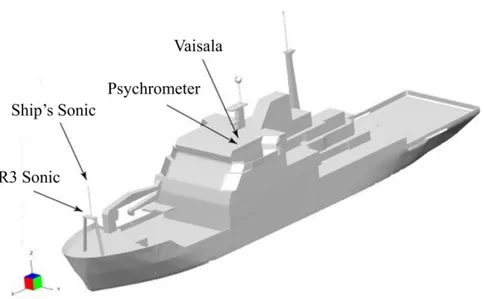
Figure 1.14 : The R.R.S. James Clark Ross geometry. The x, y and z coordinates of the instruments are shown, (Moat, et al., 2015).
A research ship named R.R.S. James Clark Ross was used for this project between 2010 and 2013. The overall length of the ship was 99 meters and the overall width of the ship measured at the widest point of the nominal waterline was 18.9 meters. 3D model of the ship was built and air flow distortion around anemometer sites were quantified with steady-state flow analysis. These cases include 0, 10, 20, 30, 50, 70, 90 and 110 degrees flow directions impacted from left and right sides of the instruments. The computational domain volume was 660 m long, 400 m wide and 150 m high for the bow-on flow. For relative wind directions at 10, 20 and 30 degrees the width was changed to 1000 m and for 50,90 and 110 degrees the width
17
was changed to 1600 m. For the wind tunnel calculations, the shape of the wind speed profile changes slightly along the tunnel. The flow around the sonic anemometer sites can suffer from air flow distortion caused by ship structure. These wind speed biases calculated with CFD software. The number of nodes within domain was around 5 to 6 million. For all scenarios, models had converged when the residuals of velocity (U, V, W), turbulent kinetic energy (K), rate of dissipation of K (E) and pressure (P) were less than 10−6. The vertical profile of the wind speed at
domain inlet was defined as a logarithmic boundary layer profile with a wind speed at a height 10 m as shown in Eq. 1.3;
U10n = u
∗
kvln ( 10
z0) (1.3) where 𝑘𝑣 is the von Karman constant (value 0.4), 𝑧0 is the roughness length and u* is
the friction velocity calculated from the Smith (Smith, 1980) drag coefficient relationship. Analysis results were presented by figures that are the best visual flow contours in the literature. Flow around the sonic anemometer which was located on the bow mast of the ship was calculated for different cases.
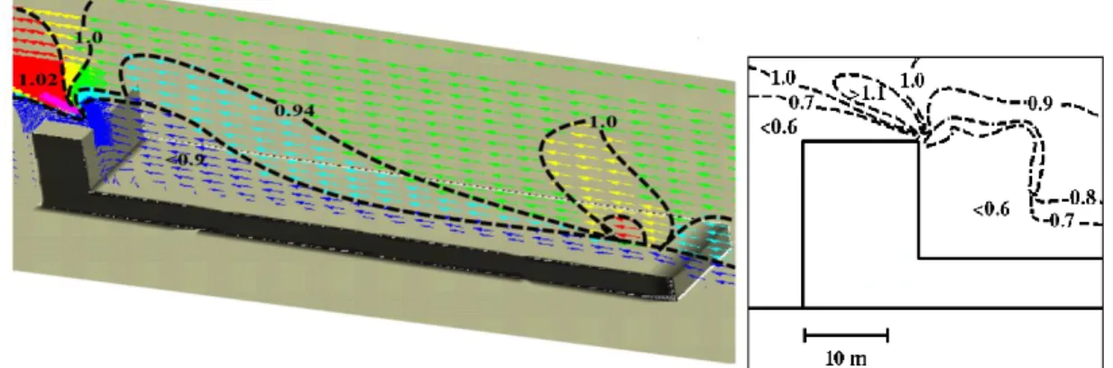
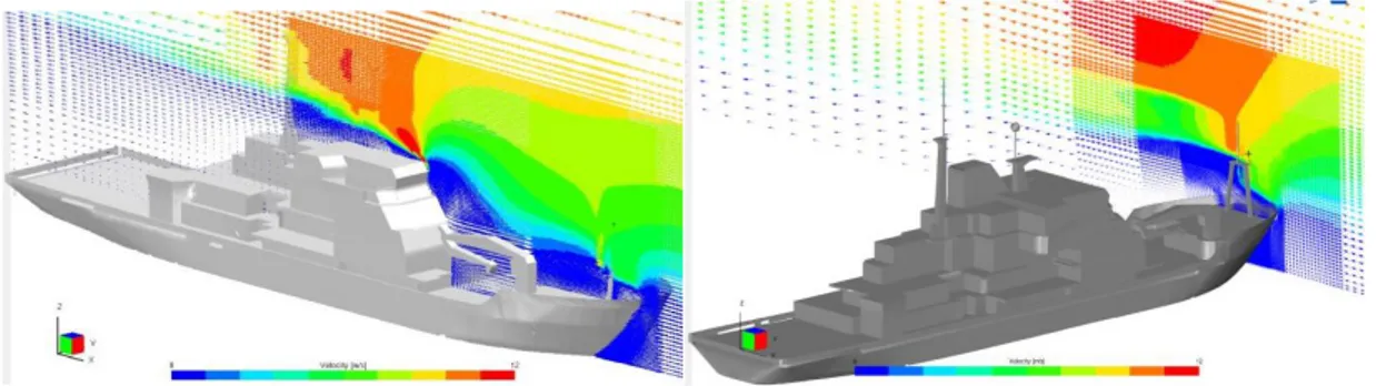
Figure 1.15 : Flow contours of bow-on and beam-on flow, (Moat, et al., 2015).
Wind speed biases were calculated for different directions and the results showed that quantifying the air flow distortion is so important to get accurate wind speed data. When the ship has bow-on flow (0 degree), the airflow at both anemometer locations was accelerated about 1% of the free stream value. The largest wind speed biases around the R3 sonic anemometer was experienced when the flow is directly from the beam of the ship. Ship’s sonic anemometer had generally smaller wind speed biases due to located well exposed position on mast.
18
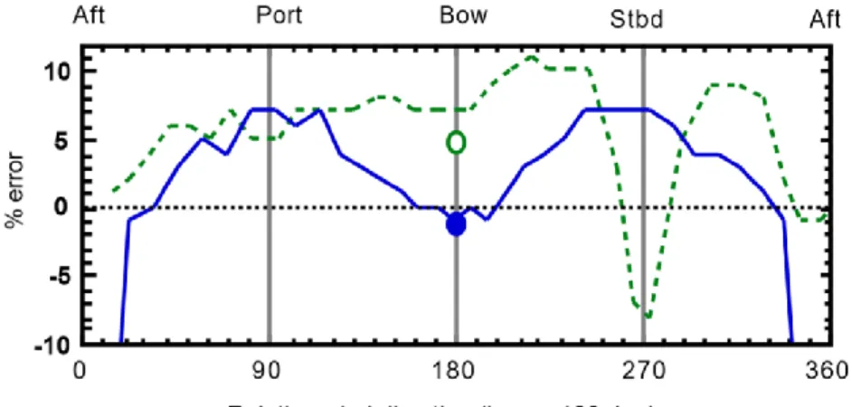
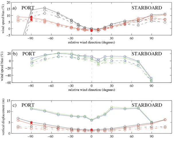
Figure 1.16 : The wind speed bias and vertical displacement at the sonic anemometer (black), ship’s anemometer (red), psychrometer (blue) and Vaisala (green). The solid lines indicate the wind speed bias using the free stream velocity from the height it originated (i.e. includes the full vertical displacement Δzt) and the chain lines indicate the wind speed bias using the free stream velocity from the height 2 seconds upstream of the anemometer location. (i.e. includes Δzt=2). The dashed lines indicate a wind speed bias at the height of the instrument. The solid symbols indicate the previous ship sonic results of (Berry, et al., 2001) at 5 and 15 m/s, (Moat, et al., 2015).
It was the most comprehensive air flow distortion study in the literature. The airflow distortion study of Berry (2001), that used 5, 10 and 15 m/s inlet flow velocities for bow and beam on flows, was developed by detailed wind speed directions. Wind speed bias has an alteration between 20% to -57% for the different directions. The study has demonstrated the ability of the CFD approaches that are employed to provide a better understanding of the airflow on research ships.
19
1.3 Offshore Wind Energy Assessment by Using Ship Sourced Data
Marine meteorological data have also been using for the wind energy assessment. In the literature there are different methods and approaches about obtaining and evaluating the data. Aim of the some wind power assessment studies is very similar with our objectives. Jimenez et al. (2007) compared WAsP (Wind Atlas Analysis and Application Program) and MM5 (Mesoscale Meteorological Model) meteorological models for offshore wind potential assessment for German Bight. In this study, two offshore (FINO and EMS), one on shore (WHV) and three island measurement stations (NR, SP and HH) were used to obtain the wind data. Data have been collected at all measurement sites from January to December 2004. Hourly mean data were controlled by visual inspection and when one of the measurement sites had an error or missing, all sites were taken out.
WAsP estimations were calculated with six different measurement data as input and MM5 was run with data from the NCEP global model as input. EMS was a lightship measurement station, and ship’s anemometers measurements were accelerated by 5-10 % because of the air flow distortion on ship structure. The comparison of the vertical wind speed profile calculated by WAsP with that measured at FINO showed rather good agreement. But, the MM5 model showed promising results with a deviation of about 4% offshore. That was a detailed local wind resource assessment and the measurement sites were examined for the effects of obstacles.
Ship mounted anemometers have also been used for determining the climate change. ICOADS has archived the wind observations from ships for years and ICOADS data set has been used in meteorological studies for climate change analysis. Tokinaga and Xie (2011) have used Wave and Anemometer based surface Wind (WASWind) method, ICOADS and in situ measurement dataset to compare wind speed observations. Sea surface wind observations and measurements are of great importance to study climate change. In this study, wind speed measured by ship mounted anemometers was adjusted with height correction if the height of anemometer was available.
20
Figure 1.17 : (a) Time series of annual numbers of ship reports in ICOADS: Instrumentally measured wind with known (black bar) and unknown (cross-hatched bar) anemometer height, visually estimated wind (grey bar), and wind wave height (solid line). (b) Time series of annual averages of monthly mean wind speed (m s21): Lindau-adjusted estimated wind (WEL, thick line), unadjusted measured wind (WM, dashed line), and height-corrected 10-mmeasured wind (WM10,thinline); WM includes both measured winds with and without HOA, (Tokinaga, et al., 2011).
Lindau Beaufort Equivalent Scale (Lindau, 1995 and Thomas et al, 2005) was used to adjust visually estimated winds. 10-m winds were estimated from visually observed wind wave heights by calibrating against height-corrected measured winds. And, night-time visual observations of wind and wave height were corrected with their averaged day-night difference. The results showed that there are close agreement between WASWind observations and satellite measurements.
In recent years, there have been some studies about wind data sources in offshore wind power assessment. Soukissian and Papadapulos (2015) focused on determining some of the Greek islands’ offshore wind potential, in which; wind data collected from buoys was compared with satellite measurements and gridded atmospheric model wind data. The maximum and minimum buoy data for different wind data
21
sources can be seen from tables in this study. All calculations were performed using the available wind speed time series from the three different data sources (buoy, satellite and gridded atmospheric model) for the same reference height of 10 m above the sea level. The relative measurement data was calibrated numerically to reduce the bias. For example, the maximum relative error (65,36%) that has been observed before calibration of Numerical Weather Prediction (NWP) model data for Santorini, was reduced to 0.64% after calibration. Results showed that different wind data sources can be analysed and compared statistically and wind power data can be obtain from different sources for offshore wind power assessment. Calibration of data sources is the most critical process for evaluating the measured wind data. After the wind data sources had been calibrated, the results come closer to each other. This is the most recent study in the literature that focuses on increasing the offshore wind energy potential assessment reliability by using buoy measurements. However, there is not any study using ship mounted anemometer data for wind energy potential assessment to the author’s knowledge.
1.4 Can We Use the Local Ferryboats to Collect Wind Speed Data In Izmir Bay?
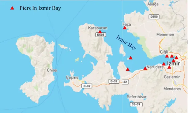
Our country especially Izmir city has a long sea shore and high wind potential in contrast to almost non-existent offshore wind potential assessment study about regions having a coast on. The Bay of İzmir, formerly known as the Bay of Smyrna, is a bay on the Aegean Sea, with its inlet between the peninsula of Karaburun and the mainland area of Foça. It is 40 miles (64 km) in length by 20 miles (32 km) in breadth, with an excellent anchorage (Wikipedia, 2016).
Ships, which almost completely have catamaran hulls in recent years, are cruising for passenger transportation throughout the Izmir Bay. Figure 1.18 shows the Bay and the points of the passenger transportation piers that are identified by the Izmir Metropolitan Municipality. Catamaran ferryboats are extremely well designed by the Ozata Shipyard Company by means of aesthetics and passengers’ comfort. Catamaran ship also doesn’t have many sharp surfaces, so the body is exposed less frictional force on cruising.
22
Figure 1.18 : Presentation of the Izmir Bay and Points of Transportation Piers, (MarineTraffic).
In the literature, research ships and VOS models were used to collect marine wind speed data; however the ferryboats cruising in Izmir Bay are catamaran type ships. Results of previous studies focused on air flow distortion caused by the ship superstructure have differences with our analyses results. Because, the ship structures and anemometer sites of the VOS models and catamaran model have no similarities. There is a gap between left and right hulls of the catamaran ferries; therefore, the ship can absorb the bow-on flow influence easier than VOS models. In this study, the catamaran ship is designed with a detailed and full scale model in contrast to that VOS were modelled with simple rectangular prisms. Research ship’s models that are used in the airflow distortion studies were more detailed than VOS models.
Catamaran ferryboats are cruising only at the inner sites of the Izmir Bay except the summer months. In summer, the catamarans have some different routes that are the extreme points of the Bay. Urla, Karaburun and Foça are the important tourism points for people who live in Izmir. People travel with modern catamaran ferries instead of land transportation to these points. Passenger ships are so active and İzmir have a great number of ship fleet; therefore we asked the question “Can we use the local ferryboats for obtaining accurate wind speed data regularly?“. We have focused
23
on quantifying the airflow distortion over local ferryboats cruising in Izmir Bay by 3D CFD analysis before collecting the data from the ships.
In this study, the ship’s mean velocity was assumed as 6 m/s (which is the ordinary cruise speed of the ship) and different wind speed in Izmir Bay was taken as 0, 5, 10, 15 and 20 m/s. Computational flow domain’s radius was 5 ship lengths, height was 5 ship heights and geometry is in the centre of flow domain. The computational domain was set at constant temperature of 25 °C. In each flow simulation, number of mesh cells was increased in specific areas. At large distance from geometry where the flow didn’t vary a great deal, the number of cells was minimized. This study has qualified and quantified the wind speed biases around the anemometer sites occurring from the ship’s superstructure. Results of this study can be used for correcting the data will be collected from ship’s anemometer and to obtain the accurate offshore wind data to determine the offshore wind energy potential in Izmir Bay.
25 2. MATERIAL AND METHODS
2.1 Description of the Catamaran and Analysis Domain
Newest local ferryboats cruising in Izmir Bay are catamaran type ships that were designed and manufactured in Ozata Shipyard Company. The maximum length of the ship (LOA) is 39 meters and the ship’s length measured at the waterline (LWL) is 38 meters. The overall width of the ship measured at the widest point of the nominal waterline (BOA) is 11.7 meters. The draft, which is the vertical distance from the bottom of the keel to waterline, is 1.40 meters. The ship has 426 passenger capacities and the maximum speed of the ship is 32 knot.
Figure 2.1 : Catamaran Ferryboat Cruising in Izmir Bay (İzdeniz).