Application of Gauss-Seidel method and singular value decomposition techniques to recursive least squares algorithm

(1)

i ^ o a .

■ M 3 S

I 3 â !

'■. DiOt ί'ί^·* ¿ •'T'-.f f"'. L.‘ <■ X juI 'íw-λ o # _{G . - i U S ¿} νΥ,.^/^Τ T .· ,y..r^ \y ¿ . D U G ^ Т М С Ч ' -J_{•A *WWJ,} _{·ί«.ί·— Οι»} _{D O} _{0 2 С Ш} jíi-LGOSlTMiví ■^1:1/ GO TOG θ η ^ :„ · іТІОО'І DG G1G.DX OF SILOEHT O - 0¿- OCiG,:;CJ

(2)

APPLICATION OF GAUSS-SEIDEL METHOD AND

SINGULAR VALUE DECOMPOSITION

TECHNIQUES TO RECURSIVE LEAST SQUARES

ALGORITHM

A THESIS

SUBMITTED TO THE DEPARTMENT OF ELECTRICAL AND

ELECTRONICS ENGINEERING

AND THE INSTITUTE OF ENGINEERING AND SCIENCES

OF BILKENT UNIVERSITY

IN PARTIAL FULFILLMENT OF THE REQUIREMENTS

FOR THE DEGREE OF MASTER OF SCIENCE

By

Atilla Mala§

(3)

<9vA

¿,oZ

(4)

11

I certif}^ that I have read this thesis and that in my opinion it is fully adequate, in scope and in quality, as a thesis for the degree of Master of Science.

Assist. Prof. Dr. Ömer MorgûIyPrincipal Advisor)

I certify that I have read this thesis and that in my opinion it is fully adequate, in scope and in quality, as a thesis for the degree of Master of Science.

Assoc. Prof. Dr. Bülent Ozffüler

I certify that I have read this thesis and that in my opinion it is full}'^ adequate, in scope and in quality, as a thesis for the degree of Master of Science.

Assoc. Prof. Dr. Enis Çetin

Approved for the Institute of Engineering and Sciences:

Prof. Dr. Mehmet Bai>

(5)

ABSTRACT

APPLICATION OF GAUSS-SEIDEL METHOD AND

SINGULAR VALUE DECOMPOSITION TECHNIQUES TO

RECURSIVE LEAST SQUARES ALGORITHM

Atilla Malaş

M.S. in Electrical and Electronics Engineering

Supervisor: Assist. Prof. Dr. Ömer Morgül

September 1991

System identification algorithms are utilized in many practical and theoretical applications such as parameter estimation of sj'stems, adaptive control and signal processing . Least squares algorithm is one of the most popular algo rithms in system identification, but it has some drawbacks such as large time consumption and small convergence rates. In this thesis, Gauss-Seidel method is implemented on recursive least squares algorithm and convergence behav iors of the resultant algorithms are analyzed. .Also in standard recursive least squares algorithm the excitation of modes are monitored using data matrices and this algorithm is accordingly altered. A parallel scheme is proposed in this analysis for efficient computation of the modes. The simulation results are also presented.

Keywords: System identification, Recursive least squares, Gauss-Seidel it erative method. Singular value decomposition

(6)

ÖZET

GAUSS-SEIDEL METODUNUN VE TEKİL DEĞER

AYRIŞTIRILMASI TEKNİKLERİNİN ARDIŞIL EN KÜÇÜI

KARELER ALGORİTMASINA UYGULANMASI

Atilla Malaş

Elektrik ve Elektronik Mühendisliği Bölümü Yüksek Lisans

Tez Yöneticisi; Yard. Doç. Dr. Ömer Morgül

Eylül 1991

Sistem belirlemesi algorirnaları, parametre tahmini, uyarlamalı denetim ve sin

5

''al işleme gibi pratik ve teorik çevrelerde yararlı olmaktadır. En küçük kareler algoritması bu algoritmalar içinde en popüler olanıdır , ancak büyük zaman tüketimi ve düşük yakınsama hızı gibi bazı aksaklıkları vardır. Bu tezde Gauss-Seidel yöntemi en küçük kareler algoritmasına uygulanmış ve oluşan algoritmanın yakınsama özellikleri incelenmiştir. Ayrıca standart ardışıl en küçük kareler algoritmasında verilerin U

3

'’ardığı modlar incelenmiş ve bu algo ritma incelenen bu modlara göre değiştirilmiştir. Bu inceleme işleminde kul lanılan hesaiDİarnalann para.el gerçekleştirilmesi için bir yöntem önerilmiştir. Deney sonuçları, her bölümün sonunda yer almaktadır.

Anahtar sözcükler; Sistem Belirlenmesi, Ardışıl en küçük kareler, Gauss- Seidel yineleme metodu. Tekil Değer Ayrıştırılması.

(7)

ACKNOWLEDGMENT

I am grateful to Assist. Prof. Ömer Morgül, for his supervision, guidance, encouragement and patience during the development of this thesis. I am in debted to the members of the thesis committee: Assoc. Prof. Dr. Bülent Özgüler and Assoc. Prof. Dr. Enis Çetin.

I would like to thank m}'· family for their constant support and all my friends, especially B. Fırat Kılıç, Erkan Savran and Taner Oğuzer for many valuable discussions. Finally, I would like to thank Miss. Ayda Soyay for helping me type the thesis.

(8)

of Qt . . . .

28 30 35 5 Conclusion 5.1 Conclusions 40 40

(10)

List of Figures

3.1 Behavior of

O

2

of GS,and standard RLS m eth od s... 23

3.2

Block GS results on

^ 3

... 24

3.3

Second example results,when GS applied to R L S ... 25

3.4 Second example results, when Block GS a p p lie d ... 26

4.1 A typical p(A) p l o t ... 32

4.2 A Parallel architecture For Algorithm

1

using N R ... 35

(11)

List of Symbols

t

: Discrete time instant.

n

: The space of real numbers.

ÁÍ

: Set of nonnegative integers. RLS : Recursive Least Squares.

SVD : Singular Value Decomposition. A R M A : Autoregressive Moving Avarage.

SISO ; Single Input, Single Output.

M IM O : Mnlti Input, Multi Output.

GS : Gauss-Seiclel Method.

N R : Newton-Raphson Iteration.

(12)

Chapter 1 Introduction

1.1 Introduction

System identification is a useful essential step in adaptive control, parameter estimation and signal processing. Recursive algorithms are derived for param eter estimation of linear systems on the basis of the least squares cost function. This well-known cost funciion could be used for derivation of recursive esti mation algorithms. Auto Regressive Moving Average (A R M A ) models cover a broad class of systems where system identification algorithms are easily ap plicable because of lineariiy . Single input ,single output (SISO) and multi input multi output (MIMO) systems could be represented by .A.RMA mod els. Recursive identification algorithms are applied by computer systems and data are generally samples of continuous time systems. In Recursive Least Squares (RLS) algorithm a ounch of computation is needed to be done during two samples of a real time process . So, there is a requirement of high speed computation, or fast con^·ergence rates to true parameters of the models for good parameter tracking and for applicability of identif

3

dng fast systems. In [3], [10], [9] convergence raies are improved in some sense, when the excitation is complete. In this thesis we propose an alternative to standard RLS algo rithm. The proposed algorithm utilizes Gauss-Seidel type sequential update rule. In this rule, the components of the parameter vector are updated sequen tially, and at each step of the update, previously updated components of the parameter vector are used. Therefore, the proposed algorithm depends on the selection of the sequence according to which the parameters are updated. If the parameter vector has

n

components, there are n! different such sequences. We note that the convergence rate of proposed algorithm depends on selection of this sequence. Hence the convergence rate can be improved by changing this

(13)

CHAPTER 1. INTRODUCTION

sequence. The Gauss-Seidel iteration method is explained in Chapter 3, for details see [1].

The excitation condition is also an important aspect in.RLS convergence behaviors. Persistent excitation will lead to a fast convergence, [4], [8], weak excitation will lead to convergence rate with order [4] and incomplete exci tation will lead to bounded errors, [11]. The excitation could be monitored by using the singular value decomposition (SVD) of data matrices. In this thesis, this monitoring is used and the standard RLS algorithm is changed accord ingly. To find the SVD of the matrices, we propose a parallel architecture. This architecture could improve the time consumption of standiird SVD algo rithms. In each block of this architecture an iterative root finding operation is done using the well-known Newton-Raphson method. VVe also give a sufficient condition to guarantee the convergence in the Newton-Raphson method.

The organization of this thesis is as follows: In Chai^ter 2 we give the re quired mathematical preliminaries for the developments done in later chapters. Some well-known stability theorems are given and matrix perturbation anal ysis techniques introduced. In Chapter 3, Gauss-Seidel method is applied to SISO, and MIMO S

3

'^stem identification schemes. Gauss-Seidel method is also applied in block fashion. The convergence properties of these algorithms are also investigated. Some simulation results are given when Gauss-Seidel method is applied to standard RLS in block or sequential fashion. In Chapter 4, SVD is used in RLS for monitoring the excitation modes and an algorithm is deri^'ed using modal behaviors. .Also a parallelization scheme, which could be used in the algorithms, is presented.

(14)

Chapter 2 Mathematical Preliminaries

In this chapter we will define the problems we consider, introduce the relevant notation and give the basic results that we use in the sequel. The systems that we consider are linear, time in’.ariant discrete time systems. These are sys tems described by difference equations of aproppriate order and are given the conventional name A R M A ;(AutoRegressive M oving Avarage models )(see below). The notations used in this research is standard; for sj'stem identifica tion, see [4], [8], for singular value decomposition, see [14], and for perturbation and stability theorems, see [12]. [15].

2.1 Recursive Least Squares Algorithm

The systems that we consider are of the following form:

y[t) = —aiy[t — l) — a‘

2 y{t —

2 )...ary[t — r)-\-biu(^t—l)-\-b

2 u(t —

2 ). .

,-f — 1)

(

2

.

1

)

where

y{t)

is the output,

u[t)

is the input of the system ; r, / > 0 are integer constants; a,-,f = l , . . . , r and 6..j = 1 ,...,/ are constant coefficients. Here, input, output and the coefficiems are assumed to be real numbers. This model is known as the ARM A model. If we let:

‘fit)

=

[ - y { t -

1 ) - y{t -

2 ) . . . - y{t - r)u{t

1 ) . . . u (i

-as the regressor vector which is a combination of p-ast inputs and observations and defining

(15)

CHAPTER 2. MATHEMATICAL PRELIMINARIES

0

= [fli ;

02

: . . . : :

¿1

:

62

: · · · :

bi]'^ell”·

as the piirameter vector, the output

y(t)

can be written as

(2.2)

where

n — r +

1 .

Hence, given we can derive

y{t)

at each time t, provided that

0

is known.

The identification problem is tentatively defined as follows:

Given system in23ut and outi^ut for a time interval, find a parameter vector which minimizes the predifined cost function.

To give a more rigorous problem definition,let us define

9

as the estimated parameter vector which has the same dimensions as the real parameter vector. Let

y{t)

=

‘■p{t)9

be the estimated output at each time f > 1. Then the problem is to minimize a suitable function of

y{t) — y{t)

with respect to

0 .

Different functions will lead to different estimation algorithms. The most widely used function is error squares cost function which is

j ( e , N)

(2.3)

where e(i) =

y{t)

— y(t), and N is an arbitrary natural number. The optimum

6

for minimizing the function

J(0,N)

is the solution of the following equation:

The matrix and the vector

Yr\f

are collections of j5ast data and outputs respectively, (i.e., : <^(2) : . . . :

Y.\· =

b ( l ) : J/(2) : .. . :

y(N)]^)·,

see [8]. Of course to find

9

we need p.seudoinverse of to exist. However by choosing N large we can achieve this task, see [8].

The above solution for

0

needs off-line computations since a batch of data are needed (i.e., collect input and past observations till time N). An alternative to this approach is updating the estimated parameters recursively using the new coming data (i.e., ?/(i)).Given an optimum estimate at time

N,

the aim is to find an optimum estimate at time iV -fl. The result is well-known Recursive

(16)

Least S quares (R L S ) algorithm, for estimating parameters. The algorithm has two update laws: parameter update and data update (covariance update ). These are.given as follows:

CHAPTER 2. MATHEMATICAL PRELIMINARIES 5

e(t) = e(t

- 1 ) +

K{t){y{t) - y,-^(t)i(t

- 1 ) )

K(i) = P(t)<p[t]

(2.4) (2.5)

(

2 .

6 )

(2.4) is the parameter update equation,(2.6) is covariance updale equation where

P{t)

is called covariance and (2.5) calculates the gain. To find

P(t)

from (2.6),the following matrix inversion identity is used :

(A

+

B C D )-'

=

A -' - A~'D(C + DAB) - ' BA~ '

provided that the required matrices are invertible. By using the above identity in 2.6, we get the following expression for

P[t)

P{t)

=

P{t

- 1) -

P{t - l)^{t){I

+

ip^{t)P{t - Vjip{t))-^i^{t)Pd -

1). To start the algorithm, initial conditions at i = 0 are needed. The initial condition

6 {T)eTV^

is chosen to satisfy ||^(0)||

< M < oo

where

M

is a finite real number, and P (0) is chosen as a symmetric positive definite matrix, usually as P (0 ) =

kI,keT^'^ ■

There are also other types of R L S algorithms which are classified by the way the covariance matrix is updated. For example ,if (2.6) is in the form

0 <

a{t) <

1

then this algorithm is called the weighted least squares with exponeritial reset ting, or if the P (t) is set to

kil,ki

is an arbitrary constant, at some tiir.e instants ¿

1

,^

2

) ·· ·) the algoi’ithm is called least squares with covariance reset ring. For a detailed exposition of the above algorithms see [4].

2.1.1 Convergence Properties of RLS

L em m a(2 .1 ):L et

y(t)

satisfy (2.2). Then, the RLS algorithm have ilie follow ing properties :

i) 11^(0 ~ > 0 where k

=

condition number of

(17)

ii) limyv-i-oo ^i=i < oo

iii) linii_^cc> 11^(0 ~ ~ ^)ll = finite

k.

Proof : See [4]

Lemma(2.1) states that the norm of the parameter error

0 = 0 — 9

stays bounded regardless of the input-output behavior, and that the measurement error e(t) is also a summable function. In the following theorem, we give a sufficient condition for

0 {t)

converge to the real parameters of the system. This could be seen easily if we define a lyapunov like function

V{t)

as ;

V{t) = 0{t)P-\t)9{t)

where

0 {t)

=

9 {t) — 9,

and use the properties of Lemma(2.1).

Theorem(2.1): The estimate

0

given by equation (2.4), converges to 0(the true parameter vector) if

lim

Xmin{P ^{t)) = oo

(2.7)

t-i-OO

where

Xmin{

2 T)

is the minimum eigenvalue of the matrix

A.

The condition (2.7) will be called the persistence of excitation condition for RLS algorithm.

Proof ; See [4].

Above theorem states that if the regressor vectors make

P~^(t)

satisfy (2.7) then regardless of the initial conditions,

0{t)

asymptotically converges to

0.

The rate of convergence highly depends on update of covariance and in standard R L S it is proportional to (|·) if input is weakly persistently exciting, [4].

Here we need to clarify what we mean by persistent excitation .

Definition: A scalar input signal is said to be weakly persistently exciting of order

n

if

N

> lim —

N-^oo N ^

t=i

u{t

+

n)

u[t

+ 1)

u{t + n)

u{t

+ 1) >

P

2 I

(2.8) where

pi > p

2 >

0.

The above definition can easily be converted to a condition on the regressors

(18)

2.2 Singular Value D ecom position(SVD)

SVD is an important tool for analyzing the modes o f the covax'iance matrix for system identification. Curly brackets cover the complex case.

Theorem (2.2): Let with rank r. Then there exists orthog

onal {unitary} matrices

V

such that

A

=

UE\r

}

E =

5 0

0 0

S = diag[a\a

2 ■. ■

cr,·)

O'! > (72 > . . ■ > ar > 0

where r =

rank{A).

P roof: See [14].Here we sketch the proof.

The elements of

S

are positive square roots of eigenvalues of ri^.4, which is positive semidefinite. Since

A^A

is symmetric and positive semidefmite, we have cr(A)C[0,oo). Let us denote the eigenvalues of

A^A

by

af, i = I , ... ,n.

Without loss of generality, we assume that cri > us > . . . > <7r > 0 =

ar+i

= . . . = (7n . Let

Vi =

'[ri...U r] and

V

2 =

[ur+i.... Un] be matrices formed by the eigenvectors of positive and zero eigenvalues, respectively. Then

S

=

diag(ai

, . . . ,

CTr)

and we have

A^AV

i

=

14

,S ',

V^A^AV

2

= 0 Then let us define

U\

as

Ut

=

AV^S

-1

and let us choose

U

2

such that

U — [Ui U

2 ]

is orthogonal. Then finall\· we will have :

U'^AV

= S 0

0 0

where

V

= [Vi :

V

2 ].

The numbers cr,· are called singular values of

A

and the columns The numbers cr,· are called the singular values of A and the columns of

U

are called the left singular vectors, the columns of

V

are called the right

(19)

singular vectors of

A.

If the matrix A is symmetric and positive definite, then the calculation of SVD is the same as the eigenvalue-eigenvector calculation of A. For, in this case

A^A

=

A^,

hence the eigenvalues of A are the same as the singular values of A. The above calculations also show that, in this case

U = V

and the columns of

V

are the eigenvectors of

A.

Thoroughout the simulations in this thesis, SVD is used. Direct computa tion of eigenvalues of

A^A

is inefficient due to machine precision, [5]. The most widely used algorithm is a two-phase algorithm proposed by Golub,Reinsch [5] . In this algorithm, the given matrix is reduced to a bidiagonal form by means of Householder transformations, and in the second phase, SVD of this bidiag onal matrix which is the SVD of the original matrix, is comi^uted by using QR alghorithm, see [5].

2.3 Stability Theorems

Let us consider the equations

y{t + l) = f{t,ty{t)) + R{t,y{t))

(2.9)

y{t + 1) ^ f{t,y{t))

(2.10)

where / :

x R ”

7?.",is such that

f{t,

0) = 0 Lipschitz function in an open subset

Ba

of

RA{i.e.. Ba

is a ball of radius

a

which is on the origin of 7?."), and i? (i,0 ) = 0

VteAf.

VVe shall consider (2.9) as a perturbation of (2.10) . Before examining the stability of (2.9) let us define some notions of stcibility

Definition (Uniform Asymptotic Stability): The solution y = 0 of (2.10 ; with initial condition

yo

is said to be uniformly asymptotically stable if

i) Given £ > 0 there exist

a.

6 —

S(e) such that for any yo being in the S neigbourhood of zero (i.e.,

B$

=

yo<IRC

|| ||||yo|||l < <5) the solution

y{t)cB,.

ii) There is a d > 0 such that for

yo(.Bs

one has limt_.oo y (0 = 0. □

DefinitionfTotal Stability): The solution y = 0 of (2.10) is said to be totally stable (or stable with respect to permanent perturbations) , if for every

e >

0,there exist two positive numbers = <5i(e) and

¿2

= <^

2

(£) such that every solution

y{t)

with initial condition

yo

of (2.10) lies in

Be

for

t >

¿

0

; provided that

(20)

and

ll/IJ < <^1

ll^(^2/W )ll < <^2 for

y(t)eB^,t > t o D .

We can now state the following usefull result.

Theorem(2.3): Suj^pose that the trivial solution of (2.10) is uniformly asymptotically stable and suppose that for some

Lr >

0

the following holds :

where

y',y"eBr

C

Ba

Then the trivial solution of (2.10) is totally stable. P roof: See [15]

And finally we have the following result.

Corollary(2.1): Suppose that the hypothesis of Theorem(2.3) is satisfied and that, for

y{t)eBa

one has ||i?(f,y('i)|| < 5'i||y(^)|| with —>· 0 monotonically. Then, the solution of the perturbed equation, (2.9), is uniformly as

3

unptotically stable.

P roof: See [15].

2.4 M atrix Perturbations

The last tool that we use in this thesis is some matrix perturbation results. A typical problem in this area is to investigate how the eigenvalues and eigenvec tors of a linear operator T change when T is subjected to a small perturbation. For a nice treatment of this and related problems see [12]. In dealing with such a problem it is often convenient to consider a family of operators of the form:

T{x) = T + xT^^'>

where a; is a small complex number, T'(O) = T is called the unperturbed oper ator and

xT^^^

is the perturbation.

(21)

Let

T,

real symmetric matrices and let x be a small complex number. If A,· are eigenvectors and eigenvalues of T, respectively, then

• OO

A,(x) = + n=l and

ipi{x) = ifi -

x5T(^V.· + - AW).ST(^V«' ~ · · ■ are eigenvalues and eigenvectors of

T (x)

= T + xT^^\

The coefficients A(” ) are given by :

\{n) ^

,n > 1,

mn

where

m

is the multiplicity of A and

p w = - ( - 1 ) " E t»i +V2 + ..-TVn = n A'l +^‘2 + ·· T^‘n+1 =^.

kj>

0 .Vj>l

Here = Pa;

=

*5'” , where P\ is a projection mapping whole space

Af

to the eigenspace o f arbitrary eigenvalue, (i.e.

T P X

=

XPX)

and

S

is given by ;

R

{0

= ( T - ( ) - '

For a detailed information about the above quantities see [12]. Another useful result is the bound for the norm ||■/,(x) —

<fi\\

which is:

where

for any

a.

- wll <

+ ,i)^||r<'V,|l.

Ipsty)i

p = ||r<“)f>|U = ||r(l).S1|.i. = ||5-oi=||

The above theorems and corollaries are the basic tools used in the thesis. Occasionally some additional results may be used, in which case they will be explained when they are introduced.

(22)

Chapter 3 Gauss-Seidel Method Applied to RLS

3.1 Introduction

We have reviewed the recursive least squares algorithm (RLS) in Chapter 1. This algorithm is known to be robust against the measurements errors [4]. The main drawback is its poor convergence behavior, since as time increases the algorithm turns itself off [3], [4]. Another drawback is the time consumption of one sweep, where sweep means a single iteration. Since in practice the sys tems in which we will use this algorithm is sampled continuous time systems, the sampling period is limited by the N}''quist rate. An efficient way of ap plying RLS to identification is to share the work of a the single sweep with p processors (i.e., p > 1) or to parallelize the algorithm. There exists a large number of efficient ¡Darallel implementations of RLS and related algorithms [2], [7]. Especially the work of Jover and Kailath is an important contribution on this area. They implement the most time consuming part of the algorithm, the covariance update, on systolic arrays. The improvement introduced is on the modification of well-known Bierman’s L D U (Lower Triangular, Diagonal, Upper Triangular) factorization of a matrix. The covariance update is in fact an LDU update problem which is solved in [6], and the modification in the paper of Jover and Kailath consist of pariillelizing the algorithm. A more systematic application schedule of parallel architectures can be found in [2]. In [2], systolic arrays are used as blocks for special purposes which are most commonly used structures in algorithms (i.e., RLS, Kalman Filtering, etc). These blocks perform; back substitution, matrix addition and multiplication, orthogonal decomposition and calculation of the schur complement[2].

In this chapter we will first give a simj^le way of parameterization of the RLS algorithm for a MIMO (Multi Input, Multi Output) system defined by

(23)

CHAPTER 3. GAUSS-SEIDEL METHOD APPLIED TO RLS 12

ARM A model. Then, we will apply a well known iteration method, which is the Gauss-Seidel iteration, for identification of SISO (single input, single output) (and MIMO.) model and examine the convergence behavior of the resultant algorithm.

3.2 Gauss-Seidel Iteration

Assume that we have the following iteration algorithm:

x{k

+ 1) =

f{x{ k))

(3.1)

where

x[k), f(x{k))eRI'.

A straightforward way to parallelize the above iter ative algorithm is assigning a processor to a component of

x{k),

and letting them compute

x{k)

in parallel. For example the processor computes

xi{k

+ 1) =

Mx{ k) )

(3.2)

which is the component of a;(/[: -f 1)· This type of iteration is called a Jacobi type of iteration. Another method is the Gauss-Seidel method(from now on abbreviated as GS). It introduces some kind of sequentalism on the calculation of the components of

x{k

+ 1). In this algorithm the recent updates of vector’s components are used to update the other components of the vector, as follows:

xi{k

-h 1) =

fi{{xi{k),x-

2 { k ) ,

... ,x„(A:))^)

X

2 {k

-f 1) =

f

2 {{^i{k

+ 1),X2(^)5...

}^n{k) f )

Xj{k

T 1) ==

fjiixiik

+ 1),X2(A- + 1

) , . . . ,Xj{k),xAk)y

) (3.3) For details, see [1]. As seen from the above equations the sequence chosen in the GS method seems to be user dependent, however, in many algorithms the sequence is predefined and the order is clearly set.

3.3 M IM O Representation for System Identification

In this section, we first give a parameterization of a MIMO system suitable for system identification. We will then apply the RLS algorithm for MIMO systems of representation

(24)

CHAPTER 3. GAUSS-SEIDEL METHOD APPLIED TO RLS ₁₃

We considei' the linear, time invariant, MIMO discrete time systems given by the following equation:

y(t)

+

Aiy{t

- 1) + . . . +

Ary{t - r) - Biu{t

- 1) + ■.. +

B;u{t - 1)

(3.4) where

tcK· ,y{t)^u{t)eRP·,

A , · , i = 1 , . . . , r, j = 1 ,___

1 .

Our aim is to find A,· ,

Bj

for i = 1 , . . . , r, j;' = ^ / using observations

y{t)

and inputs

u{_t).

Let

a‘ i _«Im _{' Ml}

. «ml · • · ^mm

, B j =

. Mnl ·■■ K , m _

, ?·

1 j

1,..., /

and let

0

be defined as

e =

(all : all : _·:

_a

_-^2

_{· ^22}

: ail : a

2_{11 · ^^21}2

(3.5) (i.e., the columns of Aj·,

i =

1 , . . . , and then the columns of B j ,

j =

1 , . . . , are placed one following other respectively)

In order to generalize the RLS algorithm of SISO systems to MIMO systems, we need to have a linear relation between the output

y{t)

and the parameter vector

9,

see(2.2). For this reason, we choose the regressors

ip{t)

as

ip{t) =

1 )

- y i { t -

1)

cR

m'^n'K rr.

(3.6)

It is easy to see that by using (3.5) and (3.6), (3.4) can be wriuen as

y{t)

= (3-7)

which is a suitable representation for identification. We will use the well-known error squares cost function

.

1 ^

0 ^ ^ ) =

2 ~

~

.(3-3)

(25)

CHAPTER 3. GA USS-SEIDEL METHOD APPLIED TO RLS 14

where

9

is the estimate of

9.

To get RLS from (3.8), let us determine a

9

which minimizes the cost function. Let us define

Y =

[?/^ (l)?/^ (2). . . and

=

[¡^{l)ifx{2

) . . .

<-p{N)Y^

then the error

E

and the cost function

J

becomes

E = Y - ^N0,

1 ^

/ =

The estimate

9

that minimizes

J

is given

(3.9) provided that the matrix is invertible. To convert (3.9) to RLS algo rithm, we assume that we have found a minimum by using — 1 errors in the cost function

J

and then we will find minimum when an additional observation comes. Note that

N N i=l ,

^^Y =

т(г)у{г)

(3-10) г= 1 If we let

P{k) =

( Ф ^ we have N izzl (3.11)

Since

P~^(k) =

Ф^Фа- and also having the definitions (3.10), we can obtain the relation

P -\ N )

=

P - \ N

- 1) +

c(N)ip^\N)

We can rewrite (3.11) as N - l

0(N) = P{ N) ( Y^ v>(z)y(<)

+ ;(Л ')!/(Л ')),

г=1

and also we have N

(

3

.

12

)

(3.13)

Y^<p(i)y(i) = P - \ N - l ) 9 { N - l ) = P- ^( N) 9i N- l ) - i f i ( N) <p^ ( N) 9( N- l ) .

(3.14) Now, using (3.14) in (3.13) we get the estimate at time

N

as

(26)

The equations (3.12) and (3.15) yield the RLS algorithm for identification of MIMO system. Here the only difference with the SISO case is that the matrix

P{N)

to be inverted is of a large size(i.e., ?n^n x

m?n).

Using the matrix inversion identity in (3.12), we obtain

p(iV ) =

P{ N

- 1 ) -

P { N - 1)^{N)[I

T

</ { N) P{ N- ) ^{ N) ] - \ ' ^ { N) P{ N

- 1 ) . (3.16) Here, the tedious computational problem is to determine the inverse of

M{t) = [IPip^{t)P{i-l)<f{t)\ t n

mxm

Under some assumptions on the system given by (3.4), a simplified RLS algorithm could be found based on the structure of

M{t)

(i.e.,

M(t)

cordd be a diagonal m atrix), see [4]. Here we did not impose a condition on

M{t).

The inversion of

M(t)

could be done in systolic array tjqDe processors which perform orthogonal decompositions and back substitutions. To clarify, let A be the matrix that we want to invert. Then A can be made triangular by multiplication of orthogonal matrices

AQ1Q2Q3 ■ ■ - Qn — U

where

_U

is upper triangular and n, the number of transformations, depends on A. Then to determine

A~^,

we invert

U

by n consecutive back substitutions, and then multiply by Q .’s, as follows:

^

= Q1Q2 ■ ■ ■ QnU

-1

This is of course not the most efficient way of performing the inversion but one which could easily be performed by systolic arrays. On conventional computer s

5

'’stems, there also exist other efficient algorithms, see[13].

This technique of MIMO identification shows the applicability of systolic arrays or parallel processing arrays to idennfication problems. The convergence behavior of the MIMO-RLS will not be dealt with since this is quite similar to SISO case.

3.4 Application of GS Iteration to RLS Algorithm

The application of GS iteration to RLS algorithm will be given in this section and convergence behavior will be analyzed in the next section. For convenience

(27)

let us consider the parameter update equation,

«(() =

§(t

- 1) +

K(t){y(t) -

-

1)).

This is an iterative algorithm. We will apply GS method on the elements o f

9

given by the above algorithm. Here the important point is the selection of the sequence to which we apply G.S. In some situations, this sequence changes the convergence behavior. For a. clear understanding, we choose the sequence,

9i{t)

=

d

2 {t) ^ 9 i { t - l) + K

2 {t){y{t) - '^x{t)9i{t) - i p2{t)9it-

1) - . . . -

^n{t)

6 n{t -

1))

On{t) = Onit

- 1) +

Kn{t){y{t) - <^i{t)9i{t) - (p2{i)92{t)

- . . . -

(pn{i)0n{i -

1 )), (3.17) for updating the elements of

9 {t).

The subindex shows that it is the associated component of the vector.

If Jacobi iteration is used in RLS, we can assign a processor to each com ponent of

6

and perform the iterations in parallel without having to wait for the result of the other processors. But in (3.17) we can see that each processor has to wait for the results of the previous processors to update its own param eter, hence the parallelism is lost. But in general, in solving linear ecpiations (i.e.A.T = 6), the GS iterations give better convergence rates than Jacobi type iterations, [1]. Here, we only prove the convergence of RLS with GS iteration. We have been unable to obtain the convergence rares of this algorithm. Hence, a theoretical comparison with RLS with Jacobi type iteration is not made.

The GS approach can also be performed in block fashion. We can partition

9 ,

K

into

k [k < n)

blocks of the form

9 = { 9 j _ : ^ : . . . : h f

p =

■■■■

R = ( ^ : ^ : . . . : ^ : d then RLS with GS iteration becomes

£i(i) = (0(2/(i) -

y y

(^¿1 “ 1) “

(28)

lk(t) = èk(t

- 1) + - . . . -

-

1))

Simulations of the block GS suggest that the convergence rate is affected by the choice of these blocks and that the error between the parameters updated by Jacobi iteration and block GS can be made small, see Figure(3.2).

3.5 Convergence Behaviors of GS Applied Algorithms

If we collect the parameters with index

t

to the left hand side of (3.17) we obtain the equation

Oi{I)

= 6>i(i - 1) +

Ki{t){y{t) -

- 1) -

y>

2 {i)

62 {i

- 1) - .. . -

<Pn(t)dn(,t -

1))

K

2 {t)MiWn(t)

+

02 (t)

=

^1

(t - 1) +

K

2 it){y{t) - f

2 (,t)d

2 {t

- 1) - . . . -

~

1))

(3.18) for GS applied algorithm. In order to write (3.18) in a compact way, we first define

E(t) =

1

K2{t)Mt)

1

and let

F{t) = I — E\t).

Then, (3.18) can be rewritten as

E{t)9(t)

= ^(i - 1) +

K{t){y(t) -

-

1)) +

F{t)0{t -

1)

or

0 (t) =

0 (t

- 1 ) +

E - \ t ) K { t M t ) -

-

1)). (3.19) Let

E{t)

= / + L, where L is a lower triangular matrix with zero elements at the diagonal. Since L ” = 0, the inverse of

E{i)

can be obtained by

(29)

In (3.19), we need

E~^{t}K(t)

which is the new gain. Hence, we need the powers of

L

multiplied by

K{t)

These can be found as follows, where the index

t

is dropped.for convenience: 0

LK

=

K

2 K^^l

+

K

2 K^if

2

0 0

L^K

L^-^K =

K - i K \ ‘~piK2'{>2 H 4 = R S2P s i ^ S2 ^S2) — {l,2,...,n—l ) H s i H s2 TSIt^S2 0 0 K n { K \ ^ l K 2 ^ 2 ■ ■ ■ K n - l ^ n - l )

The desired gain which is

E{t) ^K{t)

=

{—LyK(t)

can be expressed, using the above results as

AT

A'2(1 - R\(p-i)

An( l + ^(iii2---Sj)=(l'^’3 n-l)A5] · ·

-Ls^ips^ . . .

—

1 L)

which is ecjual to

m

K,

'

1 0

/

12(1

-

Kjift)

1 -

KiPi

K n ï i p ; { i - KiVi)

_ 0 _{n ”; ; ( i -}

_{K.v.) _}

Finally if we express

E~^

as / — Ft then (3.17) becomes

(30)

In convergence analysis we need to observe the behavior of the parameter error, which is defined

a.s Ô = Ô —

6 .

Using this definition on standard RLS we have

0{t)

= ( / -

-

1). (3.22)

If the excitation condition (2.7) is satisfied, the solution of the above error equation tends asymptotically to zero. In fact, it is known that the convergence is in the order of (1), i.e., ||6'(t)|| ~

0 ( } )

for large

t

see[4]. To examine the convergence behavior of error when GS is applied, let us write the error ec^uation as

¿(i) = U - ( / -

-1 )·

Rewriting, we have the equation

ê{t) = { I -

- 1) +

-

1). (3.23)

We note that (3.23) is a perturbed equation of (3.22). We will now check that whether the hypothesis of Theorem(2.3) is satisfied for the equation (3.22). The first thing that we have to verify is the total stability of (3.22). We will make the assumption of boundness, which is the regressor vectors produced by the system and input is bounded for all i , i.e., for some M > 0

(t)(p(t) <

M <

oo, Vi.If we let = ( / —

K(t)is^)y,

then we have

= i

i

{

/

-

-»2)11

< ||(/-A (i)'^ ’')llll»i-»2l!

< (1 + ||Aii)»>’’il)ll»i - »

2

II

(3.24)

Since

K(t) = P[t)(p{t),

using the induced T

2

nonii of matrix we obtain

< ^^LnaAPiO))

(3.25)

where we used the fact that Xmin(P~A0) A ■^mm(P~‘^(i — 1))> and hence Amai(A(i)) <

^max(P{t ~

1)), See (2.7). Using the assumption of bounded ness of regressors (3.24),(3.25), we obtain

l|/(A^l) -/(U^2)|| <

[ l + M X m o x ( P ( O ) ) m - 0 2 \ \ .

(3.26)

The inequality (3.26) gives us a candidate for A,- as 1 -|-

MX

max (P (0 )) for all

(31)

CHAPTER S. GAUSS-SEIDEL METHOD APPLIED TO RLS _,20

by(2.7), Then since 0 = 0 is a uniformly asymptotically stable equilibrium of (3.22), by (3.26) and Theorem(2.3), it is also totally stable. Now let us inves tigate the perturbed equation (3.17). We can put a bound on the perturbation as follows: iS

<

< X

Si /'m a r

< A,

(r,)jiAlt)||Mt)||||^||

(r,)A.ax(P(O))||<^(t)in|0||

Let

gt =

Amax-(ri)^mar(-P(0))||i/7(t)|p. Then, since AmasiLi) is either zero or is a multiple of

K{,

which asymptotically approaches to zero, and since regressors are bounded by assumption, we have

gt ^

0

monotonically. Hence, by using the Corollary(2.1), we conclude that 6· = 0 is also an asymptotically stable equihbrium of (3.23). We now summarize the above results.

T h e o r e m (3 .1 ): Consider the system given by (3.23), which results from the application of GS to standard RLS for SISO system. Let the persistence of excitation condition given by (2.7) be satisfied. Furthermore, assume that the regressors are bounded, i.e., there exists

M >

0, such that ||</^(t)|| <

Under these conditions, 0 = 0 is an asymptotically stable equilibrium of

(3.23). □

Theorem(3.1) can be extended easily when GS is applied in a block fashion. When the system to be identified is a MIMO system which is given in the previous section of this chapter we can still use the analysis presented above.

First thing to be done is choosing the sequence applied for GS method in the parameter update equation for MIMO case. We choose

n

blocks with elements each: For example

0 i

=

{c

11 · %1

^12 ' ^2^

: ai J

i.e. , each block 0,· is set by

A{

or

Bj.

When GS is applied, the RLS update can be done in the way shown below:

(32)

0n{t) = e^{t

- 1 ) +

- ■■■- pl{t)0n{t

- 1)).

(3.27) The equations are in same form as the (3.17) but the elements o f the matrices K and

(p

are different. We can easily see that (/?,■ is in the form

and

J/l (^ 0

yni{i

l/i(i - 0

K = Pp=[ R,^. ..K„T

ymit ^)

For the convergence of the algorithm given by (3.15), we can examine the behavior o f the parameter error

9{t)

which is

${t) — $.

By simpl}'^ subtracting

0

from both sides of (3.15) we see that error equation is

m

= (I -

m p ( t ) ) ë { t -

1) (3.28) which is the same as (3.22). From the above·equation and (3.12) it could be easily deduced that a sufficient condition for error to go zero is

—

oo.Returning to the equation where GS applied, the error equation could be written as

0{t) = { I - K{t)</{t))0{t -

1) +

TtK{t)'p^{t)~9{t

- 1) (3.29) where

% =

I - H i = , . . . n - i { I

- Ki{t)pf{t))

(3.30)

The convergence analysis is very similar to the .SISO case. First we assume that ||||s^(OIIII is bounded for all

toV.

The function, (7 —

K{t)p^ {t))^

then will satisfy the following

||7-77(07^^(011 < 1 + ||77(07’^(0II

< 1 + p^t)P{t)p{t)Mt)\\,

< 1 + ||7’(0ll?^max(7^(0)

< 1 + ||(/?(0||fA„,ai;(P(0))

(33)

CHAPTER 3. GAUSS-SEIDEL METHOD APPLIED TO RLS ₂₂

where

Lr

is the required constant of Theorem(2.3). Hence, according to the Theorem (2.3) (9 = 0 is a totally stable equilibrium point for MIMO RLS error equation, given by (3.28). Now, the perturbation term in(3.29) satisfies

\\%K{t)v>'^è\\ < ||7 ;||||W i)lP l|r(i)llll« ll

<

M^K.,{Pm\T,\\\V\\

(3.31)

It can easily be seen that the right hand side of (3.31) asymptotically ap proaches to zero, hence, by the Corollary (2.1), we conclude that ^ = 0 is an uniformly as

3

miptotically stable equilibrium point for (3.29). We summarize this result in the following theorem:

T h e o r e m (3 .2 ): Consider the system given by (3.29), which results from the application of GS to standard RLS for a MIMO sj^stem. Let the persistence of excitation condition given by (2.7) be satisfied.Furthermore, assume that the regressors are bounded, i.e., there exists

M >

0

such that ||</?(t)||,

VteAf.

Under these conditions, ^ = 0 is an as)anptotically stable equilibrium of (3.29). □

3.6 Simulations

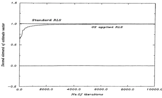
In this section we show the results obtained in the simulations done in SUN systems written in C-language In the first one a linear system is identified the system is defined b}' the difference equation

xj{t)

= 1 .7 y ( t - l)-1 .0 1 y (i-2 )-f0 .2 4 7 i/(i-3 )+ 0 .0 2 1 u (t -l)-b 0 .3 u (t -2 )-n (t -3 ). (3.32) We can define

0 =

(-1 .7 ·: 1.01 : -.2 4 7 : 0.021 : 0.3 : - 1 ) ^ and

T 'W =

[ -y{ t -

1.) :

-

2 ) :

- y { t -

3 ) :

u{t

-

1

) :

u{t -

2 ) :

u{t

- 3 ) ] ’ ’ . We take initial estimate as 0(0) = (.005 : .005 ; .005 : .005 : .005 : .005)^^ and the initial regressor as </?(0) = (.05 : .05 : .05 : .05 : .05 : .05)^' and the initial covariance as P (0 ) = 2000/6x6· The input to the system is

u (i) = 20sm (— ) + 2 0 s z n ( - ^ ) + 2 0 s ? n ( - ^ ) .

To identify the system RLS is used and GS method is applied to standard RLS using the sequence in (3.17). The asymptotic behavior of a particular element

(34)

0 .0 2 0 0 0 . 0

^

000.0 6000.0

M o . O f i.teT-atioTLS

3000.0

10000.0

Figure 3.1: Behavior of o f GS,and standard RLS methods

of

&{t),

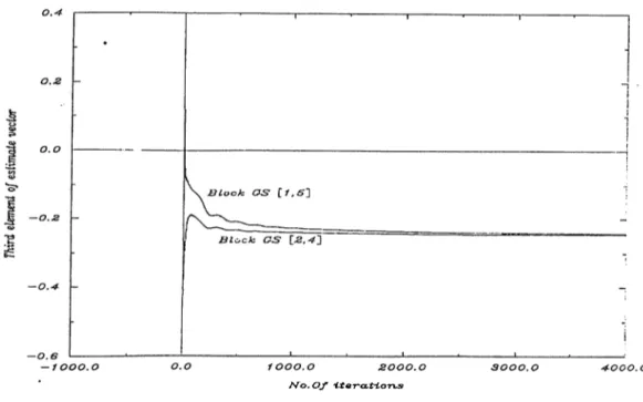
02(0) I'esulting from standard RLS and GS applied RLS are presented in Figure (3.1). In the second simulation the block GS method is used. For this purpose

${t)

is partitioned to two blocks as

We, first take

and

0(0 = (MO

01( 0

=

(01( 0

: ^2(0 )^)

02(0 =

■

U t ) ■

h {t)

:

è S ) Ÿ ·

(3.33)

Then for a second algorithm we take

^VO = (^i(O ). and

02(0 = (^

2(0

: ^VO : ^

4(0

: ^

5(0

: 4 ( 0 ') 0

The resultant behavior of 0a(O in both of the two algorithms are given in Figure (3.2).

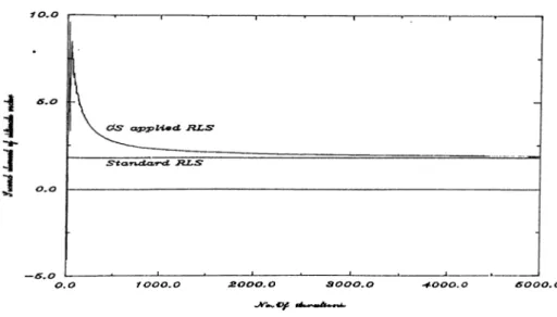
The second example we consider is a s

5

'^stem modelled by the differential eciuation

(35)

CHAPTER 3. GAUSS-SEIDEL METHOD APPLIED TO RLS ₂₄

M o . O f 'ttO'rCLirtOTLS

Figure

3

.

2

: Block GS results on

^3

The regressor and the parameter vectors are defined in the same way as we did in first example. The input is

u(i) = 20sen(— ) + 2 0 s г n ( ^ ^ ) .

The initial parameter estimate, regressor and covariance, for the iteratiA'e al gorithms, are.

= iO.8 : 0.8 ; 0.8 : 0.8 ; 0.8]^ , (^(0) = [0.05 : 0.05 : 0.05 : 0.05 ; 0.05]^^ ,

P (0 ) = 1000/.

Using the same sequencing, in the application of GS, as above we get behavior of ^

2(0

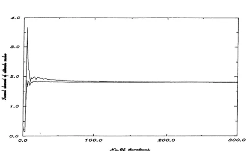
Figure (3.3).

Then we appl}^ GS in block fashion.

0(t)

is partitioned into two blocks like in (3.33), and this is done in two different ways. In the first one

0

\{i) =

■

^

2 (

1 ) ■

thetaz{t))'^,

and

(36)

z o o o ^ o

Figure 3.3: Second example results,when GS applied to RLS

In the second one

and

k ( t ) =

« ,(() =

(êi(t) : ê

4 t)

:

ê s ( i ) f .

W e display the behavior of

&

3 (t)

in Figure (3.4). The difference between these two examples is that at the second example the poles of the system is lying on the unit circle. This shows that the system may generate oscillanons. It could be seen that the convergence is poor in second example when GS applies to RLS, Figure(3.3). This could happen because of this oscillatory behavior.

(37)

CHAPTER 3. GAUSS-SEIDEL METHOD APPLIED TO RLS ₂₆

(38)

Chapter 4 Investigating RLS using SVD computations

4.1 Introduction

In this chapter we will investigate the RLS algorithm and parameter error behavior in some detail. Of particular interest is the behavior of the algorithm when the excitation is not complete or very weak so that the convergence of the estimated parameters is very slow. It can be shown that when excitation is not complete, the identification error stays bounded and some part of the error goes to zero, [11]. While this might seem to be a serious problem, that the identification error stays bounded may be sufficient for some model reference adaptive control applications, i.e., the tracking error between the plant and the model may still converge to zero, [11]. In [11] defining an unexcitation subspace by the regressor vectors, results on parameter and tracking errors are derived. Since update of the covariance plays an important role for the convergence of the algorithm, this update ecjuation is also modified. In [3], after making some modifications in this ecpiation, results show that exponentially fast convergence could be obtained, by an efficient usage of data. In [9], [10] some modifications of the RLS algorithm which avoid the turning off of the standard RLS algorithm are proposed. The turning off of the standard algorithm can be explained as follows. Assuming that the excitation condition (2.7) is satisfied, it follows that the following holds;

lim A„iar(-P(0) = 0

t-^oo

(4.1)

Since the gain

K[t)

of the RLS algorithm is proportional to P ( t ) , see (2.5), it follows that this gain asymptotically approaches to zero, hence the convergence of the algorithm also slows down.

(39)

If we investigate how the modes of increase, we can obtain some in tuition on the excitation conditions. In this chapter we propose a modification of the algorithm which is based on the excitation of modes at each iteration step and the corresponding parameters are updated correspondingly. Also, simulations suggest that even if all the ¡parameters in a sweep are not updated, asymptotically the parameter error decreases. Main motivations of proposing the above algorithms are the large time consumptions and low convergence rates of the standard RLS algorithm, (i.e. if unnecessary processing doesnot take place, time consumption decreases). If each step, instead of updating all parameters, we update the ones that are suitable in some sense at average, time consumption can be decreased. For this purpose SVD is used in covari ance update equations. Since

F(t)

is symmetric, and positive definite, SVD is equivalent to eigenvalue-eigenvector computation. The main motivation for the use of SVD can be explained as follows. Once the singular values of

P{t)

are found, we can compare these values with the previous ones, and find the directions along which the rate of change of the singular values are relatively small. Therefore we may expect small change in the parameters along these directions and do not update the parameters along them. It should be noted that the standard eigenvalue calculation algorithms are not efficient and ma chine precision dependent. This point should be taken into account when the above algorithm is implemented. Also the calculation of singular values can be reduced to finding roots of a polynomial, which has some interesting root interlacing property, see section 4.2. This property could be exploited further and a parallelization of the algorithm can be obtained.

CHAPTER 4. INVESTIGATING RLS USING SVD GOMPUTATIONS 28

4.2 Application of SVD to RLS

Since we are interested in the modes of which can be taken as the sin gular values of we apply SVD to obtain them. As is symmetric and positive definite, all singular values are positive (not zero) and decompo sition is as follows;

p -\ t ) = UtD^^U'f

d\

d'l

(4.2)

where is an orthogonal matrix and

d] >

> ... > df >

0 ,tcj\i

are the singular values. Then the covariance update equation (2.6) becomes

(40)

CHAPTER 4. INVESTIGATING RLS USING SVD COMPUTATIONS 29

■By rearranging (4.3) we obtain

(4.4) if we need to find SVD of

P~^{t)

having SVD of

P~~^{t -

1) at hand,the above equation suggests that we need to find the SVD of +

Uj_-^(p{t)(f^{t)Ut-Ui

this matrix is decomposed as

A - i +

u l M t ) ' p " { m - ^ = QtDtQj

then putting (4.5) in (4.4) we obtain

P -\ t) = H .^Q tD tQ jU l,

=

UtDl^Uf

where we set (4.5) (4.6) (4.7)

Ut

=

The update form introduced by SVD seems easy since a dyad is added to a diagonal matrix. Now let us look what changes did SVD bring to parameter update equation (2.4). Before going further, let us define

1

(4.8)

(4.9)

<i>t = Ut_j‘p{t), at = Ut_^

0 {t), -ft =

—^

Now the gain could be rewritten as

r , - ( A - _ . . r r n .X

Putting (4.9)in the parameter update equation(2.4) and using the definitions (4.8) in (2.4) we obtain

§[t) = §{t

- 1) +

-ftUt-iDt--i

4 >t{y{t) -

-

1))

= U t - \ { a t - i ' y t D t - \4> t { y { t ) — ( f t l t - i )

Then an update on a-/ will become as

at — UjUt-\{at

4-

■'/tDt-i<pt{y(t) — (j^fjt-i)

(4.10)

and since

Ut = Ut-iQi,athecomes:

a, = gf(a,_i +7,A-iA(!<(i) - 4'Iat-i))

(4 ,ir

(4.12) The vector

at

is the representation of

${t)

with respect to the basis obtained by the columns of

Ut·

In the sequel,

we

will show that, under some conditions, limi_„x, ||<5i “ -^11 = 0. Now assume that this is the case. Now (4.12) implies that, if a certain

(41)

component of

4 't

is zero, then the corresponding components of

at

and

at-i

are the same hence the parameters are not updated along this direction. In the sequel, we will show that if a certain component of

<pt

is zero, then the corresponding singular value of

P(t)

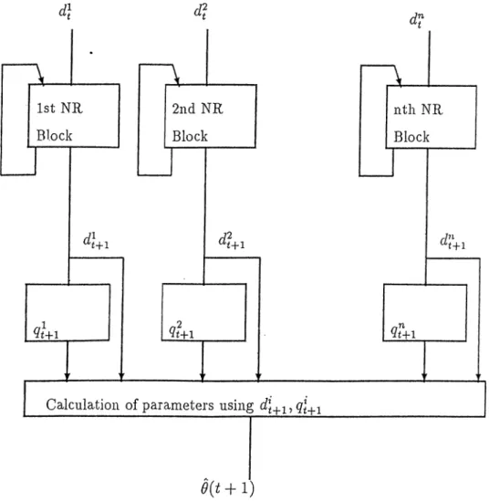
does not change. Hence, by monitoring the singular values and not updating the parameter equations along certain directions along which the singular values do not change very much, one may decrease the time consumption of the RLS algorithm.

To summarize, the use of the SVD in RLS results in the algorithm: Algorithm l:

l)Given the SVD of PjLi =

Ut-\Dt-\Uf_i

and the regressors ip(t),find the SVD of

■\-lnT

2)Update

Ut

as: hence

U t^U t-iQ t

Pf^

=

UtDr^Uj'

{B)

3) The parameter update equation is given as:

4) go to step 1.

4.3 A Parallel Implementation of SVD

In this part we will give an update scheme for covariance update (4.5). In view of (A), in implementing SVD in RLS algorithm, the crucial step is to find the SVD of the following matrix::

A + (4 1 3)

where

Dt

is a diagonal matrix with entries

d] >

> ... > df >

0

,and (/>¿

4.1

eP ” is a vector. Since the matrix in (4.13) symmetric, positive definite, finding the SVD is equivalent to an eigenvalue-eigenvector decomposition.

(42)

To find the singular values of (4.13), we first note the following:

p(X)

det(XI

- A -

= det({XI - D ,){I - {XI -

A)-V<+i<?^f+i)) =

det{XI Dt)det{I {XI

-(4.14) But, since

det{I - {XI -

A)"V«+i<P?+i) =

~

A ) " V i + i ) then (4.14) can be written as

(A -d ^ i) (A - ¿ 2 ) ■·· (A -dp )^ ^ J= i^ ^ of equivalently

p(A) = nj^.(A -

4 ) -

-

4 )

(4.15)

1=1

where c^t+i =

{w}^^,w^^i,.

. . , and

Dt = d\ag{d],d'^, ...,d f )

Remark 1: Now, assume that = 0 for some

i = l ,2 ,...,n .

We see then from (4.15) that

p{d\)

= 0, hence

dl^-^

= dj, i.e., the

i^h

singular value of

Dt+i

and

Dt

are the same. □

Since

d] > d“{ > ... > d^ >

0 ,

we have

p{dl)

=

-{w Y if{d ] - d'^){d]

- d ?)... (dj

- df) <

0 p{d¡) = -{wl,)\d^¡-d¡){d¡-d^C■■■{d^t-d?) >

0 (4.16)

,keAr

[ > 0

\i j =

2 k

Since

p{X)

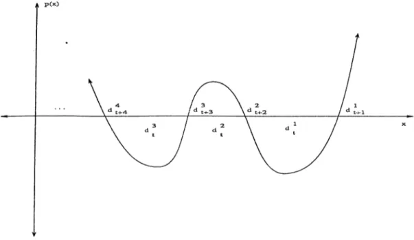
is continuous in A a typical figure for p(A) is as shown in the Figure(4.1). Then, it is not hard to see that an interlacing property between the new roots and the previous ones, as given below, holds:

4-n > 4 > 4+1 > 4 >■■■> 4+1 > 4 > o

(4.17) Furthermore, if

wj

0 for

j

= 1 ,2 ,:, n, and ifd) > d^ > : > d" > 0, then the inequalities in (4.17) can be replaced by strict inequalities. This suggest that, to find the

7

*^ root of p(A), we may choose

d^

as initial condition and apply the well-known Newton-Raphson (N R) method. A problem with these initial

(43)

Figure 4.1: A t

3

'pical

p{\)

plot

conditions is that two of them may be an initial condition of a same root. If we choose

d\, i =

1 ,... ,n

as the initial conditions in NR, to guarantee appropriate convergence behaviors, p(A) should satisfy

(

4

.

18

)

To put condition on the regressors we will write the explicit form of (4.18), using the product rule in differentiation, as

If we examine the behavior of

p{\)

at the point,

d^.

we obtain

4 4 ) = [1 - E (4.20)

i:)ik

if A: = 1 then since

p{d]) <

0, we need

p'{dl) >

0 or, if A: = 2 then since

p{d^) >

0, we need

p {df) <

0 for a general result let us partition

p {d'i)

as:

where

Application of Gauss-Seidel method and singular value decomposition techniques to recursive least squares algorithm

i ^ o a .

■ M 3 S

I 3 â !