The determinants of environmental policy stringency and the impact of environmental regulations on trade

f í c

г з

■es

C 3 S

THE DETERMINANTS OF ENVIRONMENTAL POLICY STRINGENCY AND THE IMPACT OF ENVIRONMENTAL REGULATIONS ON TRADE

The Institute o f Economics and Social Sciences o f

Bilkent University

by

AHMET ÇALIŞKAN

In Partial Fulfillment o f the Requirements for the Degree of MASTER OF ECONOMICS m THE DEPARTMENT OF ECONOMICS BILKENT UNIVERSITY ANKARA August 2000

И с

Я д

с

г

S

'

¿ О О О

I certify that I have read this thesis and have found that it is fully adequate, in scope and in quality, ^s-a thesis for the degree of Master o f Economics

—

Assoc. Trof. Syed F. Mahmud Examining Committee Member

I certify that I have read this thesis and have found that it is fully adequate, in scope and in quality, as a thesis for the degree o f Master o f Economics.

Assist. Prof. Savaş Alpay Supervisor

I certify that I have read this thesis and have found that it is fully adequate, in scope and in quality, as a thesis for the degree o f Master o f Economics.

Dr. Neil Amwine

Examining Committee Member

Approval o f the Institute o f Ecopoffiics and Social Sciences

Prof. Ali L. Karaosmanoglu Director

ACKNOWLEDGEMENTS

I would like to express my gratitude to Assist. Prof. Savaş Alpay for his supervision and patience throughout the development o f this thesis. I have also benefited from the invaluable comments of Assoc. P ro f Syed F. Mahmud and Assist. P ro f Neil Amwine. I am also indebted to Per G. Fredriksson and Paavo Eliste for providing valuable data for my study.

Although they were not here, I always found the support of my family with me during this study.

ABSTRACT

THE DETERMINANTS OF ENVIRONMENTAL POLICY STRINGENCY AND THE IMPACT OF ENVIRONMENTAL REGULATIONS ON TRADE

Çalışkan, Ahmet

Master of Arts, Department of Economics Supervisor: Assistant Professor Savaş Alpay

August 2000

In this thesis, we first focus on the relationship between stringency of environmental regulation and some conventional indicators o f economic development. We argue that this approach measures a more immediate relationship than previous studies that have concentrated on the relationship between income and emissions of pollutants. In a cross-sectional analysis, we find that the relationship between income and environmental policy stringency (EPS) is, to some degree, in line with previous findings that suggested an inverted-U type relationship between income and emissions, called Environmental Kuznets Curve (EKC). We also find that trade liberalization has a positive effect on EPS. The second part o f our study evaluates the impact o f EPS on international competitiveness in dirty industries. The analysis is done for three industries and only one o f them yields evidence for the relocation o f dirty industries to jurisdictions with lax regulation; the results were inconclusive overall.

Keywords: Environmental Policy Stringency, Environmental Kuznets Curve, Pollution Haven Hypothesis

ÖZET

ÇEVRESEL POLİTİKA SIKILIĞI BELİRLEYENLERİ VE ÇEVRE POLİTİKASININ TİCARET ÜZERİNDEKİ ETKİSİ

Çalışkan, Ahmet Yüksek Lisans, İktisat Bölümü Tez Yöneticisi: Yrd. Doç. Dr. Savaş Alpay

Ağustos, 2000

Bu tezde, öncelikle, çevre politikasının sıkılığı ile, bazı geleneksel ekonomik gelişme indikatörleri arasındaki ilişki incelendi. Bizce bu tür bir yaklaşım, gelir ile atıkların emisyonlan arasındaki ilişkiye konsantre olan önceki çalışmalardan daha öncelikli ve anlamlıdır. Kesitsel bir analiz uygulayarak, gelir- çevresel politika sıkılığı (ÇPS) arasındaki ilişkinin, daha önceki araştırmaların gelir ile emisyonlar arasında ters-U tipinde bir ilişki (Çevresel Kuznets Eğrisi) öneren bulgulan ile bir dereceye kadar uyumlu olduğunu bulduk. Ayrıca, ticaretin serbestleştirilmesinin, ÇPS üzerinde pozitif bir etkisi olduğunu saptadık. Çalışmanın ikinci bölümü, ÇPS’nın kirli endüstrilerin uluslararası rekabet gücü üstündeki etkisini araştırmaktadır. Bu analiz, üç endüstri için yapıldı ve sadece bir endüstri için kirli endüstrilerin göçüne dair hipotez desteklendi; bütün olarak bakıldığında sonuçlar belirsizdi.

Anahtar Kelimeler: Çevresel Politika Sıkılığı, Çevresel Kuznets Eğrisi, Atık Limanı Hipotezi

TABLE OF CONTENTS

ACKNOWLEDGEMENTS...

iii

ABSTRACT...

iv

ÖZET...

V

TABLE OF CONTENTS...

vi

CHAPTER I; INTRODUCTION...

1

1.1 Environmental Performance and Income... 1

1.2 Trade and The Environment... 3

1.2.1 The Impact of Trade Liberalization on The Environment... 3

1.2.2 Effect of Environmental Regulations on Competitiveness... 5

CHAPTER II: ENVIRONMENTAL POLICY STRINGENCY

AND ITS DETERMINANTS...

10

2.1 Economy-wide Variables... 12

2.2 Effects o f Trade Liberalization On Stringency... 15

CHAPTER III: STRINGENCY A N D ITS CONSEQUENCES:

POLLUTION HAVEN HYPOTHESIS

RECONSIDERED...

19

3.1 Comparative Advantage Approach... 19

CHAPTER IV: DATA AND ESTIMATION

4.1 Environmental Policy Stringency Index... 24

4.2 Other Data... 26

CHAPTER V: METHODOLOGY, RESULTS A N D

INTERPRETATION...

28

5.1

28

5.2

34

CHAPTER VI: CONCLUSION...

39

REFERENCES... 41

APPENDIX... 45

LIST OF TABLES

1. Relation o f agriculture and overall sector in Dasgupta et al. (1995). . ... 25

2. Determinants o f EPS... 31

3. Impact of EPS on ferrous metals industry... 35

4. Impact o f EPS on non-ferrous metals industry... 36

5. Impact o f EPS on cement industry... 37

1. Our approach to income-environmental quality relation... 11

2. Agriculture and overall sector relationship o f Dasgupta et al. (1995)... 25

3. Income-EPS relatio n ... 29

4. Impact o f EPS on ferrous metals industry...35

5. Impact o f EPS on non-ferrous metals industry...36

6. Impact of EPS on cement industry... 37

LIST OF FIGURES

C H A PT E R I

IN T R O D U C T IO N

Global environmental awareness has emerged since the early 1970's, marked by the Stockliolm Conference on Environment and Development in 1972. Especially in 1990's, with rapidly emerging concerns about global threats such as ozone-layer depletion and global warming, the relation between economic growth and environmental degradation has attracted the attention of both policy-makers and economists.

1.1 Environmental Performance and Income

Particularly, two lines of thought have enjoyed recent development among economists, which are: (i) the relationship between environmental quality and economic growth, (ii) trade and the environment. The former relation has been empirically modelled through emissions-income relationship by several authors. The pioneering study by Grossman and Krueger (1993) has shown an inverted U-type relationship between per capita income and emissions o f SO2 and suspended

particulates as a result of a cross-sectional econometric analysis'. The analysis was made in order to explore the possible environmental impacts of North American Free Trade Agreement. They found that, at initial levels of income, level of emissions increases-so environmental quality decreases- until a threshold level o f $4000 to $5000. After that, emissions begin to decline-and hence environmental quality increases-by further economic growth. The EKC hypothesis explained above was also verified by others: Shafik and Bandyopadhyay (1992), Shafik (1994), Selden and Song (1994), Grossman and Krueger (1995), Cropper and Griffith (1994), have

‘This inverted-U type relationship between income and emissions is called Environmental Kuznets Curve Hypothesis, (EKC) in the literature.

made similar tests with alternative indicators o f environmental degradation. Shafik and Bandyopadhyay (1992) have tested total and annual deforestation, where Cropper and Griffith (1994) have tested “rate” o f deforestation. Selden and Song (1994) has tested various air pollutants (suspended particulate matter (SPM), SO2,

NOx and CO) and found similar results; however, they found turning points substantially higher than the findings o f Grossman and Krueger (1993). Holtz-Eakin and Selden (1995) have found that CO2 emissions did not show the same EKC

pattern. Instead, CO2 emissions monotonically increased with income. Selden and

Song (1994) brought following explanation related to this result: CO2 has primarily

global effects rather than local and is more expensive to abate, as opposed to SO2,

NOx and CO. Hettige et al. (1999) have explored the income-environmental quality relation for industrial water pollution. They found that water pollution stabilizes with economic development, but did not detect an eventual decline.

A more recent study by Rothman (1998) took a consumption-based approach and criticised the previous studies that focused on production in a misleading manner. He showed that the worldwide consumption of all goods, especially the ones with higher embodied pollution show monotonically increasing functions over time, hence casts doubt on the simple EKC hypothesis. In the same study, Rothman claimed that the production o f pollution-intensive goods was transferred from developed to developing countries, and that the level of pollution-intensive consumption in developed countries did not decline.

Kaufmann et al. (1998) studied SO2 concentrations as a function o f both per

capita GDP and spatial economic activity, where the latter was defined to be the output per unit area. Spatial economic activity itself seemed to reveal an-inverted-U type relation with emissions, in the presence o f per capita GDP and its square.

A completely different approach to quantifying environmental performance was taken by Zaim and Taşkın (1999, 2000). They used an environmental efficiency index originally developed by Fare et al. (1989). In this approach, they treat the emissions and income as outcomes of a production process. In theory o f production, taking two alternative assumptions about the disposability o f bad outcomes of production, they calculated the efficiency indices for a wide set of countries. Then, they tested whether these indices show an inverted-U shape with per capita income. It turned out that they do, so they verified the EKC hypothesis using a different measure of environmental quality.

1.2 Trade and The Environment

This field of study has grown rapidly in terms o f both empirical and theoretical research. The methodological approaches to trade and environment linkage have been summarized by the literature surveys by Dean (1992), Ulph (1994), van Beers and van den Bergh (1996) and Alpay (1999). In terms o f methodology, the published work in the field may be grouped into two broad categories. The first group studied the impact of trade liberalization on environmental quality, and the second group studied the impact of environmental regulations on international competitiveness. As will be explained below in detail, trade and environment linkage is not a one-way one.

1.2.1 The Impact of Trade Liberalization on the Environment

This subject has been analyzed by various authors, often in conjunction with analyses o f growth-environment linkages. Generally, the effect of trade liberalization on environment was decomposed into three parts; the scale effect, which represents

the negative effects caused by the growth o f the size of the economic activities; the technique effect, showing the positive effects caused by innovation and cleaner production techniques; and the composition effect, showing the ambiguous effect^ generated by the changes in the bundle of goods produced by the economy. While explaining the inverted-U cuiwe obtained from income-emissions relation, Grossman and Krueger (1993, 1995), Selden and Song (1994) suggested that technique and composition effect dominate the scale effect after some threshold level o f income. A theoretical treatment of these three effects has been done by Antweiler et al. (1998). By developing a two-sector model, they distinguished these three effects and measured the magnitude of them. According to their model, the pattern o f trade was determined by the interaction o f factor endowment and income differences. They found that income gains brought about by further trade or neutral technological progress tend to lower pollution, but income gains brought about by capital accumulation raise pollution. They combined their theoretical findings with their empirical estimates of seale and technique effects, to reach the conclusion: if trade liberalization raises GDP per person by 1 %, then pollution concentrations fall by about 1 %. So, in case of sulfur dioxide, they found that free trade is good for the environment.

Some authors have studied the possible impact of trade liberalization on the environmental poliey and regulation performance o f the governments. Fredriksson and Eliste (1998) have tested whether the environmental policy stringency (EPS)^ index is related to the government transfers to the agricultural sector and strategic behavior by the producers. They suggest that there is a positive relation between government transfers to the agriculture sector and the strictness o f environmental ^ This effect depends on country characteristics, comparative advantage patterns, see

regulations on this sector. They provide this relation as a possible explanation for why observed increases in the stringency o f environmental regulations have been found to have small, insignificant, or even reverse effects on trade patterns.

Fredriksson (1999) assesses the effects of trade liberalization by a pressure group model where environmental and industry lobby groups offer political support in return for favorable tax policies. He uses this model to find equilibrium pollution tax rates. He finds that the level of political conflict falls with trade liberalization. He also shows that pollution tax decreases if the lobbying effort by the environmental lobby decreases more rapidly than by the industry lobby ceteris paribus.

A country is regarded as engaging in “ecological-dumping”, or “eco- dumping” when it gains international competitiveness in a dirty'* industry through imposing laxer environmental standards. The existence o f eco-dumping was supported by Daly (1993), Esty (1994), Dua and Esty (1997), and Esty and Geradin (1997). Xu (1999) applied seemingly unrelated regression to a system o f sectoral share equations derived from a generalised GDP function and showed that environmental factor is not a significant determinant of international competitiveness, whereas technology is. Hence he concluded that eco-dumping is not an effective strategy in this context.

1.2.2 Effect of Environmental Regulations on Competitiveness

Following Alpay (1999) we can talk o f a conventional and a revisionist school on this subject. Conventional school argues that higher environmental standards at home will deteriorate competitiveness o f domestic firms, and will

^ EPS will be explained later

'' Dirty industries are defined to be the industries that unit abatement costs exceed 1 percent o f the total cost, by Low and Yeats (1992)

relocate highly regulated industries to lax regulation countries. This idea is known as “pollution haven hypothesis” and found support from mostly theoretical papers. Pethig (1976), Siebert (1977), Yohe (1979), McGuire (1982), Palmer, Oates and Portney (1995), Simpson and Bradford (1996). Their main argument is that new environmental regulations introduce new constraints in the profit maximization problem of the firm, and this implies same or reduced profits for the firm. However, this result is not proved empirically. Moreover, many authors conducted the empirical tests of the pollution haven hypothesis and they either found no evidence o f industry relocation, or they could explain this relocation by factors other than environmental regulation differences across countries. Studies in this line include: Kalt (1988), Tobey (1990), van Beers and van den Bergh (1997). Kalt has made his test in a Heckscher-Ohlin model of international trade, whereas Tobey has used a Heckscher-Ohlin-Vanek model. Low (1991) has shown that, pollution abatement and control costs constituted 1 to 3 % of total sales and concluded that this was too low for industries to relocate to lax regulation jurisdictions, in the presence o f stronger factors like capital and labor costs. Mani and Wheeler (1999) has shown that pollution-intensive output as a percentage of total manufacturing has fallen consistently in the OECD countries and risen steadily in less-developed countries (LDC’s). However, they did not attribute this result to the pollution haven effects, because they also showed that consumption-production ratios for dirty goods remained close to unity in the LDC’s during the relevant period. Moreover, they found that income elasticity of basic industrial products in the LDC’s is high. By using a signalling approach, Bommer (1999) has shown that, relocation may not always take place beeause o f more lenient standards. Rather, for the producer, it may

be a tool o f indirect rent-seeking to convince the policymaker to refrain from a further tightening of environmental control.

The revisionist school argues that environmental policy stringency (EPS) further improves the competitiveness of domestic firms through triggered innovation. This argument was developed by Porter and van der Linde (1995)^ and was severely criticized by Palmer et al. (1995). Porter and van der Linde (1995) suggested that stricter environmental regulation forces the firms to innovate, and these firms enjoy higher productivity and hence higher profits as a result of triggered innovation. The criticism o f Palmer et al. (1995) was based on the lacking evidence for the Porter hypothesis, where Porter and van der Linde (1995) have only provided case studies in support of their argument. Theoretically, Xepapadeas and de Zeeuw (1999) show that the trade-off between environmental conditions and profits of the home industry remains, but is less sharp because o f the downsizing and modernization of the industry as a result of stricter environmental policy.

Having introduced the existing literature on the linkages between environmental performance-income and trade-environmental performance, we now mention a fundamentally different approach to the assessment of environmental performance. This approach attempts to quantify the environmental policy performance of the governments and it is pioneered by Dasgupta et al. (1995). Their methodology is based on a survey instrument that is used to assess the 1992 UNCED reports presented by 145 countries* *'. Fredriksson and Eliste (1998) have contributed to the basic data construction by evaluating the environmental policy stringency (EPS) for an additional 32 countries (only for agriculture), after the contribution of 31 countries by Dasgupta et al. (1995).

^ Thereafter called “Porter hypothesis” * The methodology is expiained in Chapter 5

In this study, we first combine these two sets o f data and construct the overall EPS index for a set o f 63 countries. Then, using this data, we conduct empirical analyses in order to get answers to three questions: First, what are the conventional economic indicators that may be determining EPS? This investigation is closely related to the income-environmental quality literature (the EKC hypothesis) that has been introduced above. In fact, we argue that this question is more critical and deserves more attention than income-emissions relation in the sense that EPS is an indicator o f the immediate response of the political authority to the environmental quality demands of the public. The change in emission concentrations is a secondary effect that occurs after income shows its effect on policy changes. We intend to focus on the shape and elasticity of EPS with respect to income to see whether strictness of regulation is related to income in the way implied by the EKC hypothesis.

Second, what are the implications o f trade liberalization for the environmental policy performance? We intend to test the effects of various openness indicators on EPS. This analysis will constitute a test of the validity o f the eco- dumping hypothesis. If we find a negative relationship between EPS and openness, this will imply that there is a motive for countries to impose laxer environmental standards if trade is further liberalised.

Our third question is whether the strictness of environmental regulation causes deterioration of comparative advantage in domestic dirty industries? If so, relocation of these industries and “pollution havens” would result. We make this analysis for three dirty industries; iron and steel, non-ferrous metals and cement. Note that, in this part o f the analysis, we take strictness o f regulation as a source of competitiveness effects, hence it is an independent variable.

The organization o f the thesis is as follows: In Chapter 2, we investigate the economic determinants of the EPS, consisting o f both overall economic variables and the openness variables. In Chapter 3, we investigate the competitiveness implications o f the strictness of environmental policy; in Chapter 4 we present our data sources. In Chapter 5 we present our results and interpretations thereof, and Chapter 6 summarizes main findings.

C H A PT E R II

E N V IR O N M EN TA L POLICY ST R IN G E N C Y AN D ITS

D ETE R M IN A N TS

Quantifying environmental policy performance has not been given adequate attention in the literature. To our knowledge, there are only two studies that shed light on this area: Dasgupta et al. (1995) and Fredriksson and Eliste (1998). Dasgupta et al. have surveyed 1992 UNCED reports in order to assess environmental policy stringency (EPS) for the overall economy, whereas Fredriksson and Eliste have evaluated EPS indices for only agriculture sector. Both have used the same methodology while constructing the indices^. Thus their indices are comparable. Dasgupta et al. have constructed stringency data for 32 countries, and Fredriksson and Eliste have done this for another 31 countries, but for only agriculture sector. In this chapter, we intend to explore the determinants o f the environmental stringency (EPS) o f the whole economy. However, the number o f countries used in Dasgupta et al. was very limited and thus needs to be extended. So, we extended the 32-country overall index o f Dasgupta et al. (1995) to 63 countries by using Fredriksson and Eliste’s (1998) study. The construction o f this data will be explained in Chapter 5.

As wc have pointed out earlier, there is an extensive literature on the relation between income and environmental quality. Some studies have only looked at pollution-income relationship (EKC hypothesis), some others have employed a larger set of explanatory variables along with per capita income, such as spatial economic activity, population density, capital-labor ratio, trade intensity, etc* *.

’ See Chapter 5 for a discussion o f the methodology.

* See Kaufmann et al. (1998), Selden and Song (1994), Antweiler et al. (1998)

Wc think that the effect of these indicators on the performance o f environmental policy and regulation is at least as important as the effects o f them on emission concentrations. Following figure will help us see this more clearly;

Wc can say that the primary force from people is the pressure on the political authority in quest of higher environmental quality. Most of the empirical studies have asked questions regarding the indirect relation between the economic indicators (mainly GDP) and emissions. However, we know that emissions are the end-of-pipe indicators of environmental quality. They are the households that put pressure on governments for them to improve environmental regulations. So, the relation between these economic indicators and policy stringency is more relevant and deserves more attention. We acknowledge the fact that, up to now, because of the lack o f data, this analysis could not be done. But now, given the partial data set, we ask the question: What arc the determinants of environmental policy stringency?

We have indicated that Dasgupta et al. (1995) have focused on some institutional measures o f socioeconomic development-like "freedom of property"-, together with real variables. Fredriksson and Eliste (1998) have used some real economic indicators like trade intensity and agriculture share o f GDP and they have found that these indicators were relevant. In this study, we intend to take a mixed

approach, where we include both institutional and real economic variables for they may both be associated with EPS.

A separate set of possible determinants o f EPS includes the variables related to trade liberalization. We wanted to investigate the effects o f trade liberalization on EPS, especially because of the extensive literature about the possible environmental effects o f the international free trade agreements.

2.1 Economy-wide Variables

The fust variable that we expect to influence EPS is the per capita income. This variable seems to be the most widely used indicator o f economic development in relation to environmental quality. Grossman and Krueger (1993, 1995), Selden and Song (1994), Shafik and Bandyoypadhyay(1992) have used it in relation to emissions, Dasgupta(1995) et al. and Fredriksson and Eliste (1998) in relation to policy stringency. The importance of income comes from the idea that, environmental quality is a normal good; so, richer people will exert more pressure on the political authority for better environmental policy, consequently better environmental quality. However, we expect that at initial levels o f income, income elasticity of stringency may be low due to the fact that poorer people are more interested in satisfying their basic needs rather than protecting natural resources. Since this information will be valuable when we will try to compare our results with the EKC hypothesis, we intend to calculate income elasticity of stringency at subsequent intervals of income. Moreover, we will try to find the functional form that best fits the income-stringency relationship.

Second variable that we expect to have considerable political impact on governments for better policy performance is the intensity o f economic activity. We

measure this variable by GDP per km . We know that every economic activity causes some harms in some way to the environment. We normalize by the area since the pressure from people will increase if the economic activity is more concentrated. This variable was called “spatial economic activity” and was used as an independent variable by Kaufmann et al. (1998). We expect that it will have a positive effect on stringency. Wc also intend to include the square of this variable, in order to observe whether it has differential effects at different income levels. In fact, we expect that it should. This conjecture is based on the fact that as countries reach a certain level of industrialization, the composition of overall output changes in favor o f service industries rather than manufacturing industries. Given that services are environmentally cleaner than manufacturing, a higher service portion of GDP implies a less marginal pollution effect of a marginal GDP per area. Consequently, a weaker effect on the environment will thrust a weaker upward stress on stringency of regulation. Hence, we expect that the sign o f the quadratic term will be negative, but do not know whether it will be significant or not. If a significant quadratic tenn comes out, this will be some support for the EKC hypothesis, implying a fall in EPS due to a cleaner environment after some threshold development level. These affluent economies liave by themselves begun to weaken emphasis on manufacturing industries, especially dirty ones'^. Hence, they do not need to increase stringency of regulations at the previous high elasticity. This is a possible explanation for the negative quadratic term of both GDP per capita and spatial economic activity. This is consistent with and can be explained by a shift o f preferences o f the individual economies as a whole. They gradually value the environment more than they value economic growth, hence find ways to get wealthier without hanning the earth. Since

’ Dirty industries are defined to be the industries that unit abatement costs exceed 1 percent o f the total production cost, by Low and Yeats (1992)

environmental valuation and awareness is not that strong in developing economies, they still have to fight with pollution via lobbying activities.

Wc acknowledge that we cannot capture the compositional effects of economic activity by employing the variables GDP per capita and GDP per area. There are many countries in the World that relies upon resource industries, or in which a significant portion of the total output is from service industries. These industries yield quite large amount of income, but do not generally require high levels of capital, and generally do not pollute much (See Antweiler et al. (1998)). To get rid o f the differences in the embodied capital in total income, we will use capital- labor ratio, measured by the accumulated capital investment per worker, (KAPW) as an explanatory variable for EPS.

Antw eiler et al. (1998) provide empirical evidence that more capital intensive industries arc more polluting industries. Given this information, we expect that capital intensity variable will have a positive effect on EPS.

This variable is not only important only for its implications for the structure o f an economy. It also has a strong interaction with trade liberalization. Factor endowment hypothesis states that a country exports the good that embodies a higher percentage of the factor that is abundant in that country. Capital and labor are the most widely used factors of production in an economy. Capital-labor ratio and indicators oi‘ opcnness-which will be explained later- arc crucial variables in the sense that further openness together with factor endowment considerations have important effects on international trade.

We intend to include the urban ratio of the total population, URB, as an explanatory variable in our regressions. As we know, industrialization process

involves ever increasing population in cities. If we look at the history o f the modern environmental movement beginning with the early 70s, we observe that the political pressure from environmental interest groups has been improved by the rising urban population in many developed and developing countries. The possible association o f urban population ratio with EPS has two different sources. First, more crowded cities made cleaning o f air, water and land more important. This is especially true for local pollutants that have immediate effects. The increasing threat o f pollutants have come from both accommodation and manufacturing activities around cities. Secondly, “environmental consciousness” has been improved by the process o f urbanization. The mechanism o f this increasing awareness was through the help o f mass media. Mass media has been a strong instrument of environmental interest groups. They have effectively used it on government and on industry representatives. The strength of the mass media comes, of course, from the highly organized, highly educated city population. We predict that both dimensions o f urbanization have positive relation with EPS.

2.2 Effects of Trade Liberalization on Stringency

Environmental implications of trade liberalization have been analyzed extensively during 1990s, especially because o f the influential free trade agreements such as North American Free Trade Agreement (NAFTA) and the Uruguay Round. There is a growing literature on both theoretical and empirical approaches to possible implications of freer global trade on the resources o f individual countries and the world. Up to date, the focus o f the research has been on the implications o f freer trade on the emissions of various pollutants, such as SO2 and CO2. Many theoretical

papers on the issue suggested that environmental policy differences across countries together with higher capital mobility drove pollution intensive industries to the countries with lax regulation. This hypothesis is called the “pollution haven hypothesis” and has been defended by some theoretical papers'®. However, Grossman and Krueger (1993), Tobey (1990), Jaffe et al. (1995) empirically tested this hypothesis and detected no significant effect o f policy differences on trade flows. Since this hypothesis is related to the consequences o f EPS rather than its causes, we will analyze this issue in detail in Chapter 3. Our focus here is the effect of openness itself on the EPS. We argue that openness to international markets, or the absence thereof, may have effects on the level o f ES in a country.

Now, let us try to explain why openness should be effective on the EPS. In this respect, first argument is based on export markets. We know that, less-developed countries (LDCs) chiefly export to developed, high-income countries, where high- income countries themselves chiefly export to again high-income countries. The exporting LDCs must meet the stricter environmental standards of high-income importing countries (or groups of countries like European Union). For this purpose, exporting firms o f the LDCs must shift to cleaner production processes. Given the assumption that exporter firms are also, in general, biggest producers in those LDCs, these shifts to cleaner processes reduces the negative pressure from producer lobbies on the EPS. This makes the tightening of the environmental standards easier for the policymakers. For developed economies, they chiefly export to other developed economies and there is no impact on production techniques induced by exports. For the portion o f their exports to LDCs, the environmental standards o f their own will

10_{See Chapter 1 for examples.}

prevent them from exporting dirtier products to LDCs. Hence the overall effect of further trade liberalization on the EPS should be positive".

A second argument in favor o f the suggested positive impact is as follows. Currently, there are global pressures on exporting countries for the ratification of international environmental agreements. Some agreements ban imports from non- signatories*^. This pressure will exert positive thrust on ES o f exporters as a whole.

A counter-argument to the above scenarios has been suggested by a number o f scholars; this is known as “eco-dumping hypothesis”. This hypothesis suggests that competitiveness in international markets will force governments to relax their ES in the hope of gaining competitive advantage through lowering costs. However, many empirical studies in the literature show that abatement costs are a small percentage (1 to 3) of the total costs o f production (Low (1991)), so they may not have real effects on competitiveness. We will test whether increased competition in the world market in the form o f further trade liberalization has a negative effect on EPS.

Various indicators of openness to international markets have been suggested by several authors. The most widely used one is the ratio of the sum o f exports and imports to GDP (called as trade intensity, O Pl). We too, intend to use this variable while testing the impact of openness on EPS. Since there may be some information that we cannot capture by trade intensity, we have to use other indicators of openness. We intend to adopt the following indicators suggested by Sachs and Warner (1995);

1. Black market premium in foreign exchange markets over 1980s (BMP).

" For more on tins discussion, see Birdsall and Wlieeler (1992) Case of Korea can be found at: htlp://ci.mond.org/9615/961519.html

2. Average level o f tariffs on imports over 1985-1988 (TAR). It is the own-import weighted average tariff rate on capital goods and intermediates.

3. Coverage of quotas on total imports during 1985-1988 (QUO). It is the own- import weighted non-tariff frequency on capital goods and intermediates.

C H A PT E R III

ST R IN G EN C Y AND ITS CONSEQ UENC ES: PO LLU TIO N

H AV EN H Y PO TH ESES REC ON SIDERED

In this chapter, we intend to inquire into the possible consequences o f EPS on the economies. The analysis made here evaluates the effects o f EPS on the comparative advantage o f “dirty” ^^ industries o f the economies. This analysis will yield valuable results in the assessment of the “pollution haven hypothesis”, which suggests that dirty industries will migrate to the countries with laxer regulation.

3.1 Comparative Advantage Approach

Here, we intend to measure the effects o f the ES on the comparative advantages o f the respective countries. The first step here is to find an indicator of comparative advantage o f a specific country for a specific industry. For this purpose, we adopted the Revealed Comparative Advantage (RCA) devised by Balassa (1965,1979) and used by Low and Yeats (1992). RCAij of a specific country i for good j is the ratio of the share o f exports of good j of country i in its total exports, to the share o f world exports of good j in the world total exports. If this ratio is greater than unity, this is generally interpreted to mean that the country is at a comparative advantage in the trade o f the product, since the industry’s share in the country’s exports exceeds its share in world trade. This seems to be a relevant measure of the competitiveness in an industry o f a specific country. It is also comparable in the sense that it uses standard criteria for measurement. We intend to use the following

See Chapter 1

model to measure the possible impact o f the EPS on the competitiveness o f the countries in a specific industry j:

DRCAij = c (l) + c(2)*EPSi i = 1,..,63 countries (1)

In the above equation, DRCAij represents the difference in the RCA o f country i in industry] between 1982 and 1992'"*. This model tests the hypothesis that, whether competitiveness o f industry j has decreased between 1982 and 1992 for the countries with a higher EPS. A negative coefficient on EPS will imply the verification o f the above hypothesis. Assuming that investment decisions are based on comparative advantage and capital is mobile enough across countries, above result will constitute some empirical support for the “pollution haven hypothesis” .

One should recognize the assumption in the above model that EPSj is constant during the relevant period. In fact, rather than its constancy, we need to only rule out changes in EPS that are not proportionate across countries. If all the countries have increased their EPS by the same percentage, this will not change the relative stringency o f each country with respect to all others. So, there will not be an incentive for an industry to relocate to another country. For the purpose of analysis, we have to make this assumption, since we want to obtain the sign and the magnitude o f differences in competitiveness o f an industry in different countries while holding their policy strictness constant. We consider that ten years is short enough for constancy o f the EPS, but long enough for dislocation of industries to more profitable areas. The following are our justifications for these assumptions:

We can say that investment decisions made by firms are much more dynamic than legislation and enforcement o f government regulations. Red-tape in bureaucracy, political controversies, industry lobby activities always make

''' Tlie selection of 1992 is due to the fact tliat EPS data was constructed from UNCED 1992 reports. The selection o f ten years will be c.\plaincd.

environmental regulations hard and time-consuming to enforce and implement. Environmental awareness does not develop in a matter o f ten years, yet only developing it does not guarantee reforms in environmental policy.

As expressed earlier, a negative and significant coefficient on EPS will imply that more stringent economies have had a deteriorating weight in dirty industries. A positive and significant coefficient, on the other hand, will imply two possible results:

1. The widely accepted anti-thesis o f pollution haven is the factor- endowment hypothesis. It suggests that a country exports the goods that embody a higher percentage o f the factor that it abundantly has. We know that capital and labor are the most widely accepted factors o f production and industrialized, high-income countries are endowed with more capital and low-income countries with more labor. We also know that capital-intensive industries are generally dirtier (Antweiler et al., 1998). So, the hypothesis suggests that further trade will induce high-income, high- EPS*^ economies to specialize in capital-intensive, dirtier industries. So, a positive coefficient will imply that factor-endowment hypothesis is dominant in determining comparative advantage patterns.

2. The second explanation to an improving competitiveness emerges as possible empirical evidence to the “Porter hypothesis” . Porter, in a theoretical paper, has shown that, in some cases, stricter environmental regulation at home increases competitiveness of domestic firms through innovation. The mechanism is as follows: Tough environmental regulation in the form of economic incentives can trigger innovation that increases a firm’s competitiveness in the long-run, which would not

15

Tlie point Uiat liigh-income economies have also high ES values was established by Dasgupta el al. and Fredriksson and Eliste, as explained in Cliapter 1

be the case without the regulation. Eventually, this effect may outweigh the short-run costs o f the regulation (Porter and van der Linde (1995)).

In case a positive relation comes out of the regression o f eqn.(2), we have to assess whether this result comes from a factor-endowment basis, or from the innovation suggested by Porter, or from both. To test the possible influence of capital-labor ratio (KAPW) on the comparative advantage o f dirty industries, we can devise the following model:

DRCAij =

c(l)

In the above equation, DRCAy represents the difference in the RCA of country i in industry) between 1982 and 1992 as explained before, and DKAPWj represents the percentage change in the KAPW of country i between 1982 and 1992. In this model, we are attempting to measure the influence o f the changes in the “capital abundance” on the changes in the RCA. This is exactly a test o f factor endowment hypothesis for dirty industries, remembering that dirty industries are also capital intensive. We expect a positive relationship under the validity o f the factor endowment hypothesis. Given that we have only two alternative explanations for a positive relationship in (2), an insignificant coefficient from (3) should imply that the positive thrust on competitiveness comes from innovation and productivity changes o f the firms in economies with stricter-regulation, and not from an increased relative capital abundance.

A significant positive coefficient on KAPW difference will lead us to a verification o f the factor-endowment hypothesis. However, this will confiase us about a possible “Porter” effect. A further influence on comparative advantage of innovation and productivity may or may not exist. Since we do not have detailed data on the technological superiority o f some economies over others, (of course, we must

have quantified data for a very wide set o f countries for this purpose) we cannot empirically assess the Porter effect in this analysis.

C H A PT E R IV

D A TA A ND ESTIM A TIO N

4.1 Environmental Policy Stringency Index

The most important information that constitutes the core of our analysis is the environmental policy stringency (EPS) index for a wide set of countries. As we have expressed earlier, we developed this data from the studies of Dasgupta et al. (1995) and Fredriksson and Eliste (1998). Fredriksson and Eliste have adopted the methodology of Dasgupta et al. (1995). While constructing the data, Dasgupta et al. (1995) surveyed the reports presented by a large number o f countries to the UNCED 1992. Since the reports were prepared according to a standard reporting format imposed by UN, they were comparable across countries. Dasgupta et al. used a multidimensional survey that assesses the state of;

"(i) environmental awareness; (ii) scope o f policies adopted; (iii) scope o f legislation enacted; (iv) control mechanisms in place; and (v) the degree o f success in implementation"'^

Twenty-five survey questions are assessed in a 4x5 matrix, and one o f 0, 1,2 values are entered for each entry, where these values indicate low, medium and high performance, respectively. The matrix consists o f the four environmental aspects: Air, Water, Land and Living Resources. On the other dimension, there are five activity sectors; Agriculture, Industry, Energy, Transport and the Urban sector. Then by summing up all the 500 entries for each country, overall index is obtained.

For the purposes o f our analysis, we extended the 32 countries o f Dasgupta et al. to a larger set for a more healthy statistical analysis. Also, the above set of

16

Tlie survey instrument is available in Dasgupta et al. (1995) paper.

countries was mostly consisting of low-income countries and did not include many countries that belong to high-income group. At this point, we recognized that the relation between agricultural and overall indices is quite strong.

Figure 2

Note: EPSDAS and AGRDAS stand for tire EPS indices o f Dasgupta ct al. (1995) for agriculture sector and overall sector, respectively.

Table 1

Note: EPSDAS and AGRDAS stand for tlie EPS indices o f Dasgupta et al. (1995) for agriculture sector and overall sector, respectively.

Included observations: 32

White Heteroskedasticity-Consistent Standard Errors & Covariance EPSD AS=C( 1 )+C(2)* AGRDAS

Coefficient Std. Error t-Statistic Prob. C (l) 51.89328 21.81992 2.378252 0.0240 C(2) 4.983269 0.170076 29.30021 0.0000

R-squared 0.937751 Mean dependent var 541.3438

Adjusted R-squared 0.935676 S.D. dependent var 199.6584 S.E. o f regression 50.63758 Akaike info criterion 7.909849 Sum squared resid 76924.94 Schwarz criterion 8.001458

Log likelihood -169.9636 F-statistic 451.9376

Durbin-Watson stat 1.265256 Prob(F-statistic) 0.000000

As it can be observed from the graph and OLS regression results above, the interaction between agriculture index and overall index is quite significant and no outliars are observed. Note that the coefficient o f 4.98 quite reflects the five activity sectors. Given that we also had the stringency values for agricultural sector for another 31 countries from Fredriksson and Eliste (1998), we could estimate the overall environmental policy stringency (EPS) values for this second set o f countries from the linear equation we obtained above. So, we were able to extend Dasgupta et al. Data set to 63 countries through this estimation*’ .

4.2 Other Data

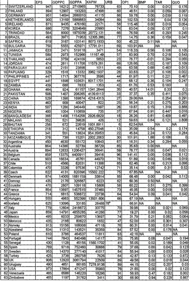
The next set o f data we required was the output data. GDP per capita expressed in 1985 international prices (Chain Index) was obtained from Penn World Tables (PWT). The collection and estimation o f the PWT data is described in Summers and Heston (1991)**. To get rid o f temporary fluctuations in the income, we took three-year averages (1990, 1991 and 1992). The other data obtained from this source includes population, trade intensity, and capital stock per worker. Trade intensity is calculated as the ratio o f the sum o f imports and exports to total GDP. Capital stock per worker (KAPW) was calculated as the cumulative, depreciated sum o f past gross domestic investment in producers durables, nonresidential construction, and other construction. KAPW data was missing for 20 countries of our set of 63 countries. We estimated this data from the "World Tables 1992"*^. We took the values of the Gross Domestic Investment expressed as percentage of GDP for the 1981-1990 period. Then we accumulated the investment values and depreciated with

’’ Tlie stream o f EPS values for 63 countries and otlier data are available in Table A l in Appendix. The PWT data are available in revision 5.6 from Uie NBER ftp site at ftp://ftp.nber.org/pwt56/

19

See references

20% annual rate of depreciation. We picked the 20% rate as an average that we estimated from the method applied by the PWT, where they used differential rates for machines, construction equipment, etc.

To calculate the GDP per area variable, we obtained the necessary area data from A.S. Banks' "Political Handbook o f the World 1998". The urbanisation data was obtained from Table 31 of "World Resources 1992-93" published by World Resources Institute. For missing countries in World Resources, we resorted to World Development Indicators 2000, published by the World Bank^°.

The openness indicators other than trade intensity were taken from Sachs and Warner (1995).

For the comparative advantage analysis conducted in this study, we obtained the export data from 1985 and 1993 issues of the “International Trade Statistics Yearbook” published by the United Nations. These sources give exports o f each country by the three-digit SITC commodity code. The 1985 and 1993 yearbooks also included data o f 1982 and 1992 that we used for our analysis.

Tills source can be accessed tlnough tlie website:

http://www.worldbank.org/data/databytopic/databytopic.html

C H A PT E R V

M E TH O D O LO G Y , R ESULTS AND IN T E R PR E T A T IO N

5.1 Results for Determinants of Stringency

Our search for the determinants o f environmental stringency includes the test of many explanatory variables, which are defined below:

EPS is the environmental stringency index,

GDPPC is the GDP per capita, and GDPPCS is the square of it, GDPPA is the GDP per area, and GDPPAS is the square of it, KAPW is the capital labor ratio,

URB is the urbanization rate.

OPl is the trade intensity, (exports+imports)/gdp,

BMP is the black market premium in foreign exchange markets (can also be viewed as an indicator of financial liberalization);

TAR is the tariff coverage for imports, QUO is the quota coverage

As it was explained before, the first seven variables are economy-wide variables and the last four variables measure the openness o f a country. When we analyzed the correlation matrix for the explanatory variables o f the above variables, we observed that GDP per capita variable is highly correlated with the capital per worker (KAPW)^*. To avoid the multicollinearity problem, we decided to drop the KAPW from our model.

The BMP variable will be included as a dummy variable in our model so that the value 1 indicates there is no positive or negative premium in foreign exchange

markets and 0 otherwise. The dummy will be denoted D l. This implies that the countries with D l= l are financially liberalized.

One o f our aims about the development-EPS relationship is the analysis o f the relation at different income ranges. For the purpose o f specifying the relevant categories o f income, we decided to look at the following graph that shows the relation o f per capita income with EPS;

While we are making the classification, we took several criteria into consideration. First, we were careful to make an even distribution o f points to each category. Second, when we analyzed the above figure, we realized that we could talk o f three different slopes of income-EPS relation for three income groups. It appears that until like $2000, the slope seems quite high. After 2000, slope seems to be lower for the middle-income group, which we may categorize as until, like $8000. After $8000, it seems that the variation in the high-income group decreases. That

Tlie correlation matrix is presented in Table A2 in Appendix.

implies a convergence among these countries. The groups that we suggest are as the following; Income Poor Middle-income High-income $0-$2000 $2000-58000

$8000-To see whether the behavior of the intercept and slope of the income-EPS is significantly different in these groups, we intend to include two dummies, D2 and D3 and two variables GDPPC*D2 and GDPPC*D3, respectively. D2 is designed such that the value 1 is entered if the country is poor and 0 otherwise. D3 is designed such that 1 is entered if the country is middle-income and 0 otherwise.

In our initial regressions where we included all the variables listed at the beginning o f the section as explanatory variables, the followings were observed: The variables GDPPCS, GDPPA, GDPPAS, URB, TAR, QUO appeared to be insignificant. Given this information, we suggest our model:

EPS = C (l) + C(2)*GDPPC + C(3)*OPl + C(4)*D1 + C(5)*D2 + C(6)*D3

+ C(7)*GDPPC*D2 + C(8)*GDPPC*D3 (3)

The results o f the OLS regression are below;

T a b l e 2

Included observations: 51

Variable Coefficient Std. Error t-Statistic Prob.

GDPPC 0.020328 0.005979 3.399804 0.0014 O Pl 0.673604 0.289538 2.326475 0.0247 D1 563.9357 88.38368 6.380541 0.0000 D2 270.4018 38.78760 6.971345 0.0000 D3 278.0646 38.18439 7.282155 0.0000 GDPPC*D2 0.082801 0.031541 2.625170 0.0119 GDPPC*D3 0.026877 0.009329 2.881083 0.0061

R-squared 0.950312 Mean dependent var 623.3333

Adjusted R-squared 0.943536 S.D. dependent var 221.0263 S.E. o f regression 52.52051 Akaike info criterion 8.049281 Sum squared resid 121369.8 Schwarz criterion 8.314434

Log likelihood -270.6225 F-statistic 140.2539

Durbin-Watson stat 1.897653 Prob(F-statistic) 0.000000

While we are dealing with cross-sectional data, the first thing that we fear o f is the heteroskedasticity problem. To get rid o f this problem, we tried "White's correction for heteroskedasticity" while doing regressions, which is available in the Eviews package. White has derived a heteroskedasticity-consistent covariance matrix for calculating standard errors and t-statisties. (See Halbert White "A Heteroskedasticity-Consistent Covariance Matrix and a Direct Test for Heteroskedasticity", Econometrica 48, 1980). The White covariance matrix is given by;

T

T - k

{X'Xr\Y^u,^x,x'){X'Xr

(4)

where T is the number of observations, k is the number of regressors, and ut is the least squares residual. When we conducted the same regression using the above correction tool, we observed very close results to the presented results. So we concluded that the problem o f heteroskedasticity is not present in our case and kept the original results above.

The first result from the results is that the per capita income has a strong and positive impact on EPS. This result verifies the findings o f Dasgupta et al. (1992) and o f Fredriksson and Eliste (1998). As expected, as people gets richer, they demand better envirpnmental regulation. Secondly, the trade intensity (O Pl) variable and financial liberalization dummy (D l) has a strong and positive effect on EPS. This implies that more openness leads to a better environmental policy performance. This result is a clear rejection of the eco-dumping hypothesis that claimed a "race to the bottom" as a result of freer trade. Thirdly, our classification o f countries on income basis and the designated intervals seem to be relevant, evidenced by the significant coefficients for both the intercept and the slope variables. This implies that the designated income groups show significantly different characteristics in the three groups in terms o f income-EPS relationship. The slopes for these groups are given below: Slope Poor 0.103 Middle-income 0.047 High-income 0.020 32

Looking at the slopes above, we can talk o f a "convergence" in the high- income group in the sense that the variation in terms of EPS within this group is low compared to other groups. The sensitivity of EPS to income among the middle and especially low- income group is high. This implies that there is a significant potential for better environmental policy performance within the poor and middle-income group. If we take the positive strong effect of trade liberalization and financial liberalization into consideration, we may expect that many countries in low and middle-income groups will experience improvements in terms o f policy performance.

Our second result that openness is good for environmental policy performance is also supported by Antweiler et al. (1998). This result can be based on following arguments:

a) As a result o f the shift of production processes of the LDCs to cleaner ones in order to meet higher environmental standards o f the importer high-income countries, enhancement o f policy performance becomes easier for LDCs.

b) The international environmental agreements seem to have a real positive effect on world-wide policy performance. Especially, practices like blocking exports from non-ratifying exporters proves to have a detectable effect on ES.

c) Openness seem to increase the awareness on global environmental matters.

5.2 Impact of Stringency on Competitiveness

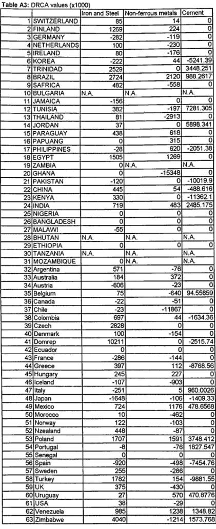
To be able to obtain results from our differential revealed comparative advantage model expressed in Chapter 2 (eqn. 2), we need to choose some dirty industries. Low and Yeats (1992) listed forty three-digit SITC code industries as dirty industries. These were the industries that incurred pollution abatement and control expenditures o f greater than or equal to 1 per cent o f their total sales in 1988 in US. They include all three-digit products in SITC 67, SITC 68, and SITC 69 and fourteen other three-digit industries from different classes. We picked three industries from the list; ferrous metals (SITC 67), non-ferrous metals (SITC 68), and cement (SITC 661). We calculated RCA values for each country and for the years 1982 and 1992. We took the difference and scaled DRCA by multiplying it by 1000, while doing regressions'. The results for the three industries are given below:

Tlie DRCA values are available in Appendix A3.

Ferrous metals ('iron and steeH STTC 67 Table 3

Note: The data point for Dominican Republic was an outlier, so was dropped from data set.

Included observations: 59

Excluded observations: 4 after adjusting endpoints

White Heteroskedasticity-Consistent Standard Errors & Covariance DRCA67=C(1)+C(2)*EPS

Coefficient Std. Error t-Statistic Prob. C (l) 999.9195 344.3194 2.904046 0.0052 C(2) -1.008972 0.453893 -2.222928 0.0302

R-squared 0.051409 Mean dependent var 374.2712

Adjusted R-squared 0.034767 S.D.dependent var 914.5937 S.E. o f regression 898.5543 Akaike info criterion 13.63488 Sum squared resid 46021790 Schwarz criterion 13.70531

Log likelihood -483.9465 F-statistic 3.089101

Durbin-Watson stat 1.411550 Prob(F-statistic) 0.084188

EPS

Figure 4

Note: Tlie data point for Dominican Republic was an outlier, so was dropped from data set.

Non-ferrous metals. SITC 68 Table 4

Note: Since Ghana and Chile showed as outliers, we dropped tlieir data points.

Included observations: 56

Excluded observations: 7 after adjusting endpoints

White Heteroskedasticity-Consistent Standard Errors & Covariance DRCA68=C(1)+C(2)*EPS

Coefficient Std. Error t-Statistic Prob. C (l) 341.8829 294.1927 1.162105 0.2503 C(2) -0.493072 0.343501 -1.435430 0.1569

R-squared 0.022289 Mean dependent var 31.69643

Adjusted R-squared 0.004183 S.D. dependent var 682.9430 S.E. of regression 681.5130 Akaike info criterion 13.08369 Sum squared resid 25080840 Schwarz criterion 13.15603

Log likelihood -443.8039 F-statistic 1.231052

Durbin-Watson stat 2.210671 Prob(F-statistic) 0.272119

EPS

Figure 5

Note: Since Ghana and Chile showed as outliers, we dropped tlieir data points.

Cement. SITC 661 Table 5

Included observations: 58

Excluded observations: 5 after adjusting endpoints

White Heteroskedasticity-Consistent Standard Errors & Covariance DRC A 661 =C( 1 )+C(2)*EPS

Coefficient Std. Error t-Statistic Prob. C (l) -934.2082 1195.092 -0.781704 0.4377 C(2) 0.661826 1.451629 0.455919 0.6502

R-squared 0.001699 Mean dependent var -521.1034

Adjusted R-squared -0.016128 S.D. dependent var 3289.214 S.E. o f regression 3315.632 Akaike info criterion 16.24668 Sum squared resid 6.16E+08 Schwarz criterion 16.31773

Log likelihood -551.4522 F-statistic 0.095299

Durbin-Watson stat 2.270605 Prob(F-statistic) 0.758691

According to the above results, countries o f higher ES seem to lose competitiveness in ferrous metals industry. This deterioration of competitiveness is implied to exist at 3 per cent significance level. This result implies that this industry

has escaped from strict-regulation to lax-regulation countries during 1982-1992 period, supporting the pollution haven hypothesis. However, tests with other two industries do not support the same pattern. Statistically, these tests did not yield a significant result, with very low probabilities to reject null hypothesis of no relation. Despite being insignificant, the last two tests yielded positive coefficients, hence created doubt about the result obtained in the ferrous metals industry. Another point that leads us to inconclusiveness is the very low R-squared values from all three tests. At best, we can say that for some industries, strict-regulation countries may have lost competitiveness during the relevant period^^.

22

Here, one should bear in mind tlie assumption of constant relative EPS during tlie relevant period.

C H A P T E R VI

C O N C L U S IO N

In this study, we investigated three topics. The first was to explore the relationship o f the strictness of environmental regulation (EPS) to the more conventional indicators o f development like per capita income, spatial economic activity, capital-labor ratio and urbanization rate. Our approach in this study was novel in the sense that we explore the impact of these variables on the environmental policy performance, which is a more immediate impact than their impact on the emissions. The results showed that per capita income has a very strong and positive relation with EPS. Per capita income seemed to embody all the information that is inherent in the other explanatory variables. This result verified the results o f Dasgupta et al. (1995) and Fredriksson and Eliste (1998). In addition to these findings, we classified countries on an income basis and found that different income groups show significantly different characteristics in the income-EPS relationship. According to our classification, the $0-$2000 low-income group seemed to have a higher potential in terms of EPS improvement. The middle-income group seemed to have a lower response of EPS for a marginal increase in income, relative to low- income countries. Lastly, high-income countries seemed to be concentrated within the group. This implies that we observe a pattern o f "convergence". While we increase income per capita, the variability o f EPS within the respective group decreases.

The second part of the analysis was to assess the effects of trade liberalization on environmental policy performance. Positive significant effects of both trade intensity variable and the financial liberalization dummy on EPS were found. So, the eco-dumping hypothesis that countries impose laxer environmental standards in the