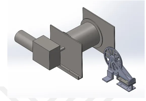
Fatigue resistant design of an aerostat's mooring station
Tam metin
Şekil


Benzer Belgeler
architectural design (traditional media: paper-based drawings and physical scale models; and digital media) are analyzed in terms of their capacity to support dynamic
Tensile strength tests, hardness tests, toughness tests and fatigue crack growth tests have been applied on HPA welded samples, GMA welded samples and base
Such problems can be discussed for each particular structure. However the general reason for not removing columns and beams from a structure is the rule, which forms
The guideline recommends a clear hierarchy of public spaces con- nected by the spatial and visual linkages, diversity of uses for different user groups, local building
Aziz N esin’in bitm eyen enerjisi sü rüyor v e bir yanıyla Avrupa, bir yanıy la Asya, bir yanıyla Orta Asya, bir y a nıyla Karadeniz, Bir yanıyla Akdeniz, bir yanıyla
Şarj istasyonu veya uyumlu Welch Allyn Vital Signs cihazı, termometredeki ayarları değiştirmek için Welch Allyn Service Tool ile birlikte kullanılabilir.
Frequency Samling Method.
Limit states design (called by AISC as Load and Resistance Factor Design (LRFD).. Working Stress Design (or Allowable Stress
