Weld Defect Categorization from Welding Current
using Principle Component Analysis
Hayri Arabaci1
Electric-Electronics Engineering Department Selçuk University Konya, Turkey
Salman Laving2
Mechatronics Engineering Department Selçuk University Konya, Turkey
Abstract—Real time welding quality control still remains a
challenging task due to the dynamic characteristic of welding. Welding current of gas metal arc welding possess valuable information that can be analyzed for weld quality assessment purposes. On-line monitoring of motor current can be provided information about the welding. In this study, current signals obtained during welding in the short- circuit metal transfer mode were used for real-time categorization of deliberately induced weld defects and good welds. A hall-effect current sensor was employed on the ground wiring of the welding machine to acquire the welding current signals during the welding process. Vector reduction of the current signals in time domain was achieved by principle component analysis. The reduced vector was then classified by various classification techniques such as support vector machines, decision trees and nearest neighbor to categorize the arc weld defects or pass it as a good weld. The proposed technique has proved to be successful with accurate classification of the welding categories using all three classifiers. The classification technique is fast enough so it can be used for real time weld quality control as all the signal processing is carried out in the time domain.
Keywords—Arc weld defects; feature extraction; PCA; classification techniques; on-line monitoring
I. INTRODUCTION
Welding is an integral process in manufacturing in the metal industry. Gas Metal Arc Welding (GMAW) is usually chosen over other welding techniques due to its various advantages. A few major advantages are high productivity, can be used for automation, is mobile and the welding can be carried out from various angles and positions. Due to its exponential growth and vital importance in the industry, the need for evaluating any defects present on the welded parts arose. A lot of research has been carried out to overcome this challenge but due to the complexity of the physics involved in arc welding [1] the challenge has not been successfully overcome. The complexities arise from the various variables/parameters that define the dynamic welding process such as gas flow rate, welding intensity, welding speed, electrode feed rate, material composition, arc length, weld seam geometry etc. All these variables are interrelated by a highly non-linear and interdependent process [2], making it difficult to come up with a valid theoretical model to define the process. Therefore, many researchers in the area have focused on studying the welding parameters individually or combining a few together to get feedback on the final weld quality.
Several undesired scenarios can appear during the welding processes which may directly affect the quality of the final welds. Some of the known factors of weld defect and irregularities during GMAW are; Instantaneous short circuits, failure of arc re-ignition and wire feed rate variations [3]. These factors, if kept under steady control, can lead to achieving a good final weld. Other factors which cannot be directly controlled like contamination and environmental conditions in the welding area need to be kept optimal to ensure quality welding. Commonly used off-line techniques to identify welding quality include destructive (macrographs) and non-destructive testing like x-ray, ultrasounds, penetrant liquids, magnetic particles, etc. [4]. These off-line techniques, although being accurate, have many drawbacks so research work has mostly focused on developing an on-line sensing and welding path determination by using feedback and adaptive control [5]. On-line monitoring of the welding process reduces the effects of the uncontrollable factors and also saves on the otherwise resource consuming quality control inspection. Several sources such as welding sound, voltage signal, current signal, power, weld-pool image, electric arc are found to have a correlation with weld quality [6].Therefore the most commonly used methods of on-line quality inspection derive from the use of welding voltage and current [7], welding sound [8] and high-speed photography [9].
Multiple studies have been carried out to analyze the sound produced for the purpose of on-line weld defect. It is common knowledge that the human welder combines both audible sound and vision to control the welding process [10]. The knowledge of the behavior of acoustic signals generated during the welding process is important for inspection of the consistency of the process [11]. The sound signals produced during GMAW carry information about the transfer mode, behavior of the arc column and the molten pool [8]. A mathematical relationship that relates the sound produced during the welding, the arc voltage and the welding current was formulated by [12]. A study by [13] showed that the short circuit transfer mode of the GMAW produces discernible sound which makes it easier to capture and analyze compared to the other two modes; Globular mode and spray mode. Despite the vast research on this area, industrial use of sound signals for on-line quality monitoring of GMAW is still not realized. This is due to the fact that in the industrial environment back ground noise is a great hindrance to the acquisition of the welding sound. Usually research is carried out in laboratories using welding trolleys or a moving
workpiece that is usually not the case in the industries. The background noise in these laboratories is from the shielding gas and the welding machine which is not a hindrance since their magnitude is very low compared to the actual welding sound [14]. In addition, the sound signals require some signal processing before being able to use which makes the on-line defect detection slower. Some of the basic signal processing includes filtering the sound signal in time domain and then converting the filtered signal to frequency domain for further processing [15].
High-speed photography is another method some researchers have used to develop on-line weld defect detection. It is not a very common technique due to the fact that it is expensive, can be affected by splatter which can damage the acquisition equipment which is closely placed to the welding torch and requires high bandwidth for acquisition and processing. Measuring the arc voltage and welding current is a common method researchers have been using for defect detection in the welding process [7]. This method is simple and relatively reliable and most of the signal processing can directly be carried out in the time domain. Welding equipment usually keep one of the parameters constant; constant voltage or constant current welding equipment. It is common to take the parameter that is variable for weld quality control purposes. Several time domain processing techniques have been suggested by researchers. Some have successfully used welding voltage or welding current to detect a defect in the welding process. Control charts have been used by [16] on the welding voltage to identify porosity in the final weld. They confirmed their study using radiographic test. Hilbert–Huang transform and time–frequency entropy was used by [17] on preprocessed current signals to estimate the stability of short-circuiting GMAW. The author in [18] proposed using regression modeling using all the three parameters; sound, current and voltage to predict two main weld quality measures; welding defects and bead shape factor. A technique of Wavelet packet coefficients of current signal in back-propagation Artificial Neural Network (ANN) was used by [19] to monitor weld defects in Pulsed Metal Inert Gas Welding. The authors achieved an error rate of 11% using this technique. ANN together with PCA feature extraction was successfully employed by [20] to monitor arc-welding systems. They presented several examples of weld seams that showed that, once the ANN has been properly trained, it can efficiently discriminate different welding defects, lack of penetration and gas flow reduction among others. Many similar approaches have been used in research and theoretically the results are promising. However, a universal on-line system that will detect weld defect and categorize them immediately is still lacking. Some approaches require too much time to process and give results which may be a hinder for on-line control. Some approaches tend to be complex so implementation cannot be realized. For example acquiring voltage, current and sound at the same time complicates the system and may lose versatility where it may work for some applications and be erroneous on others.
This study presents a technique for detecting a weld defect and categorizing the cause of the weld defect. Current signals
were acquired from deliberately induced weld defects as well as from good welding. The weld faults were induced by:
Deliberate fast welding
Welding carried out without shielding gas
Deliberate slow welding
Increasing the wire feed rate
Decreasing the wire feed rate
The captured current signals in time domain are then processed using PCA for vector reduction. The reduced vector samples are then divided into train and test samples for classification. A total of three classifiers were used to identify which classifier is the fastest and most accurate. This technique aims to reduce the complexity of the system, be versatile and give results fast enough so they can be used for on-line defect detection and categorize the cause of faulty welds.
II. EXPERIMENTAL PROCEDURE
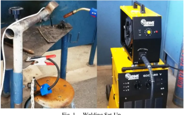
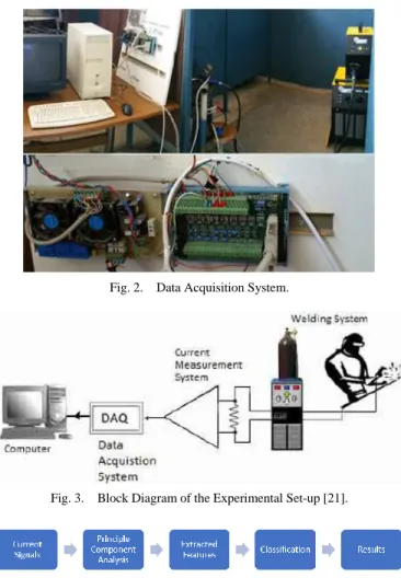
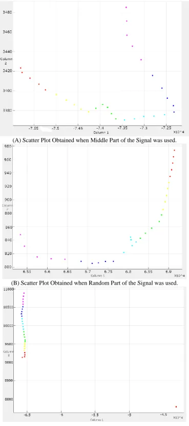
Standard industrial, constant voltage, welding equipment, OZEN GDC360 V was used in this study. The experiments were carried out on mild steel plates which were 4 mm thick using an electrode wire with a diameter of 1.0mm. The shielding gas used was a mixture of Argon (80%) and Carbon 20(%). The welding current is sampled at 20 kHz from a Hall effect current sensor using a data acquisition card. The photograph of the welding set-up and components used are shown in Fig. 1 while the data acquisition system photograph is shown in Fig. 2. The block diagram of the used experimental system is given in Fig. 3. An experienced welder carried out the welding and varied the parameters for deliberate faulty welding. The parameters for a good weld are shown in Table I. Eight runs for each welding class were made with a run time of approximately 5 seconds for each run. feature extraction and classification were made for each data. Flow chart of the technique used in this study was given in Fig. 4.
Fig. 1. Welding Set-Up.
TABLE I. WELD CLASS DATA ROW PLACEMENT IN A MATRIX
Parameter Value
Wire Feed Rate 350 cm/min
Fig. 2. Data Acquisition System.
Fig. 3. Block Diagram of the Experimental Set-up [21].
Fig. 4. Flow Chart of the Technique used in this Study. III. EXPERIMENTAL RESULTS AND DATA PROCESSING The Current signals of each weld run acquired on the data acquisition system were exported in excel format to a PC for the processing. Each signal had around 100,000 samples so the first part of the processing was to truncate the signals to 10,000 samples. To get accurate results, the truncation was done randomly on different parts of the signal. Several truncation runs were made from different parts of the signal each time to ensure legitimacy of the results. The plots on Fig. 5(A-F) show the signals truncated from sample 30,001 to 40,000 from the first test runs of the different weld types plotted versus time.
(A) Current Signals Obtained from Fast Welding.
(B) Current Signals Obtained from Welding without Shielding Gas.
(C) Current Signals Obtained from Good Welding.
(D) Current Signals Obtained from Slow Welding.
(E) Current Signals Obtained from Fast Wire Feed Rate Welding.
(A) Weld Obtained when no Shielding Gas was used.
(B) Picture of a Good Weld.
(C) Weld Obtained when the Welding Speed was Increased.
Fig. 6. (D) Weld Obtained when the Wire Feed Rate is reduced. The rising and falling of the welding current in a well-defined pattern usually signifies a good weld. This can clearly be seen on Fig. 5C where the peaks are in a good pattern and well spread out with little difference between peak gaps. A photograph of the good weld is shown in Fig. 6B. Notice the few peaks in Fig. 5A; the welding process was too fast therefore short circuits took place far apart resulting in a bad weld. Fig. 6C shows a photograph of a fast weld where it can be seen that the material deposition is less. Rapid peak currents can be noticed on the weld carried out without shielding gas as shown on Fig. 5B. Fig. 6A shows the weld carried out without using shielding gas. The porosity of the final weld can be seen. With a fast wire feed rate shown on Fig. 5E, the electrode is vigorously fed to the workpiece leading to constant contact (short circuit) therefore the current is almost always peaked. From Fig. 5F it can be deduced that with a slow wire feed rate, there is little metal deposition with time therefore short circuits that are very far apart. Fig. 6D shows the corresponding photograph where the weld is basically just splatter.
From Fig. 5(A-F) it is clear that welding current signals possess valuable data that can be used to categorize weld defects. Statistical methods like Peak to Peak, Standard Deviation, Root Mean Square, Skewness and Kurtosis etc. could directly be used on this raw data to identify the weld defects with some success. But in the real industrial environment such deliberately induced weld defects would not exist. The variation of the short circuit peaks may be little when a defect comes across so statistical methods may be left wanting. Therefore Principal Component Analysis (PCA) was chosen for this study. PCA not only finds the variance in data, but it also carries out dimensional reduction which gets rid of
redundant data. This is especially useful when using a classifier to classify the data.
A. Principle Component Analysis
Principle Component Analysis (PCA) is one of the most important methods used in pattern recognition and compression. In the works of [22], fault detection applications in industries using PCA have been presented. The authors reviewed cases where PCA was successfully implemented in the various industries coming up with a conclusion that it is feasible to use PCA for successful fault detection. Despite this fault detection success in the industry, PCA is more commonly known for its role in facial recognition applications. Many researchers on facial recognition techniques choose to use PCA for feature extraction from the facial images. In PCA method, the 2-Dimensional face image matrices are transformed into a Dimensional vector [23]. Since signals are already in a 1-Dimensional vector, it simplifies the data processing even further as there is no need to concatenate the vector before applying the PCA method. The main steps to be carried out in the PCA approach are summarized below:
1) Standardize the scale of the data into d-dimensional vector (d is the different classes of data).
2) Compute the covariance matrix for the data. The covariance matrix is the scatter matrix.
3) Obtain the Eigenvectors and Eigenvalues from the covariance matrix or alternatively perform Singular Vector Decomposition. Eigenvectors and Eigenvalues exist in pairs: every eigenvector has a corresponding eigenvalue. An eigenvector can simply be thought of as a direction while an eigenvalue is a number showing how much variance there is in the data in that direction.
4) Sort the eigenvectors in order of decreasing eigenvalues and choose k eigenvectors with the largest eigenvalues to form a d by k dimensional matrix W in which every column represents an eigenvector. W is our new projection matrix
5) Finally, the projection matrix is used to transform the samples onto the new subspace.
In our case, we had 8 test runs for each of the 6 weld groups (5 faulty welds and 1 good weld). To make processing much faster only the last 5 test runs were used for PCA. Therefore, a total of 30 different classes were used for the feature extraction each having 10,000 samples. The data was standardized into one matrix of 30 by 10,000. The first five samples were of Fast welding followed by No Shield Gas welding. The Good weld data was on classes 11-15 followed by Slow welding, Rapid Wire Feed weld and Slow Wire Feed Rate weld at classes 26-30 as shown in Table II.
Then the covariance of this matrix was computed. This resulted in a 10,000 by 10,000 matrix. This was followed by obtaining the eigenvectors and corresponding eigenvalues from the covariance matrix and choosing 100 eigenvectors from the 10,000 obtained with largest eigenvalues in a descending order. Projecting onto the subspace leaves us with a matrix of just 30 by 100. Taking fewer Eigenvectors will increase the speed of the process but may affect the performance. Taking more eigenvectors would lead to slow processing with a slight
increase in performance up to a certain point. In our case 100 was found to be optimal. The data at this point was ready to be used for classification.
TABLE II. WELD CLASS DATA ROW PLACEMENT IN A MATRIX
Type of Weld Row Placement
Fast Welding 1 to 5
No Shielding Gas Welding 6 to 10
Good Welding 11 to 15
Slow Welding 16 to 20
Fast Wire Feed Welding 21 to 25
Slow Wire Feed Welding 26 to 30
Classification is a supervised learning approach in which the computer program trains from the data input given to it and then uses this training to classify new observation. The most commonly used classifiers are;
1) Naive Bayes Classifier 2) Support Vector Machines 3) Decision Trees
4) Boosted Tress 5) Random Forest
6) Artificial Neural Networks 7) Nearest Neighbor
For this study SVM, Decision Tress and Nearest Neighbor classifiers were used.
B. Support Vector Machines
Support Vector Machines (SVM) classifier makes use of the special function called the kernel, with which the experimental data set is converted from the original space of characteristics into the higher dimension space with the construction of a hyperplane that separates classes [24]. SVM is one of the most popular classification systems in data mining and pattern recognition applications, due its high classification rates [25]. It gives very good results in terms of accuracy when the data are linearly or non-linearly separable. When the data are linearly separable, the SVMs result is a separating hyperplane, which maximizes the margin of separation between classes. If data are not linearly separable, the algorithm works by mapping the data to a higher dimensional feature space using an appropriate kernel function [26]. C. Classification Results and Discussion
The Projection vector was tested with the three mentioned classification techniques. To decide on which runs of the weld classes to choose for training and testing, two methods can be used; Cross Validation and Holdout. Holdout simply takes a percentage of the data for training and tests the rest with that trained data. This method is good for large data sets. Since each weld class had just five runs in the reduced vector, using holdout method was not feasible so cross validation method was used. Cross validation method selects a number of divisions to partition the data into. Each division is then held out in turn for testing. The classifier trains each division using data outside the division and the data to be tested is within the division and the average test error over all division is
calculated. In this way all data is used for both training and testing thus classifying more accurately. This method takes longer to classify compared to holdout but the overall efficiency of the results is better. The classifier results are presented in three different figures to give a good idea of the accuracy of each classifier and show which weld class was misclassified. The three figures show Percentage Accuracy, Confusion Matrix and Scatter Plots.
(A) Scatter Plot Obtained when Middle Part of the Signal was used.
(B) Scatter Plot Obtained when Random Part of the Signal was used.
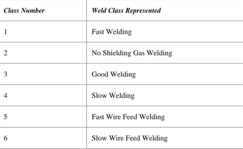
Fig. 7(A-C) shows the scatter plots of the projected vector data. The different color dots represent the weld types. A scatter plot gives an idea of how successful PCA was on a certain data set. Well spread out data means that the feature extraction was successful and high success rates in classification. Data points of different classes close to each other on the scatter plot will usually lead to a less accurate classification but that also depends on the classification algorithm used as well. Figures 8A and 8B show the scatter plot from PCA conducted on the middle parts of the signal. The data is well scattered and the features from the different weld types are discernible. Fig. 7C shows the scatter plot from PCA conducted on the first part of the signals, which is from sample 1 to 10,000. Although the different weld types can be differentiated, the feature points are not so well spread out compared to when the middle parts of the signal are used.
Fig. 8 (A-D) shows the percentage accuracy of the three classifiers used on the projected vector from different parts of the signal. Fig. 9A and 9B, whose corresponding scatter plot is 8A and 8B, are the results of when the middle part of the signal was used. Fig. 8C resulted from the same projected vector as 9B but in this case Quadratic SVM was used instead of Linear SVM to see the effect on the final accuracy. Fig. 8D, whose corresponding scatter plot is Fig. 8C, is the accuracy when the first part of the signal was used. From the accuracy plots it is clear that using the first parts of the signal can result in lesser accuracy. This may be due to the fact that during the first few seconds of the welding process the process is not very stable and the current readings may fluctuate abnormally. It is also clear that k-nearest-neighbors is by far more accurate and reliable for classification on our dataset. It achieved 100% accuracy in all runs except for the first part of the signals where an accuracy of 90% was realized. SVM is also a reliable classifier for our data set and using Quadratic SVM increased the accuracy as depicted from Fig. 9B and 9C. Decision Trees classifier performed poorly and is unreliable for our data set. Overall speed of all the classifiers was very fast. In a matter of milliseconds we had the accuracy results. Generally the accuracy results portray the success of using PCA on current signals for weld defect detection.
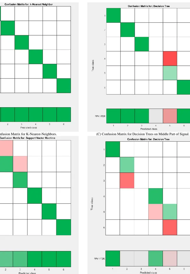
Fig. 9 (A-D) shows the confusion matrix of the classifiers. A confusion matrix is a table that is often used to describe the performance of a classifier on a set of test data for which the true values are known. As the green shade gets darker the percentage accuracy increases while darkening shade of red implies increasing percentage error in classification. The Legend for Confusion matrix is presented in Table III. Fig. 9A shows the confusion matrix of the k-nearest-neighbors classifier (almost all runs from different parts of the signals had the same result). The k-nearest-neighbors classifier accurately categorized the weld defects and can tell whether it was a good weld or not. Fig. 9B shows confusion matrix of the SVM classifier when the first part of the signal was used. The classifier could not tell the difference between fast welding, no-gas welding and good welding in some of the weld test runs.
It misclassified 2 good weld runs as being no-gas weld runs and 2 no-gas weld runs as being fast weld runs. When other parts of the signals were used SVM had 100% accuracy in categorization. Confusion matrix for decision trees is shown in Fig. 10C and 10D. Decision tree classifier struggled in categorizing the welding types. In some cases, it totally misclassified the weld types as can be seen from Fig. 9D where it entirely misclassified the good weld and slow wire feed rate weld. Overall accuracy of categorization by Decision Tree was around 80% when the whole signal is considered.
(A) Classification Accuracy when Middle Part of Signal was used.
(B) Classification Accuracy when Random Part of Signal was used.
(C) Classification Accuracy when Quadratic SVM was used Instead of Linear SVM.
Fig. 8. (D) Classification Accuracy when First Part of Signal was used. TABLE III. LEGEND FOR CONFUSION MATRIX
Class Number Weld Class Represented
1 Fast Welding
2 No Shielding Gas Welding
3 Good Welding
4 Slow Welding
5 Fast Wire Feed Welding
(A) Confusion Matrix for K-Nearest-Neighbors.
(B) Confusion Matrix for SVM on First Part of Signal.
(C) Confusion Matrix for Decision Trees on Middle Part of Signal.
IV. CONCLUSION
In this paper, an attempt was made to categorize weld defects from current signals using PCA and a suitable classifier. Current signals were obtained from deliberately defected welding and good welds. Defected welding was obtained by either changing the welding speed, changing the wire feed rate or carrying out welding without shielding gas. Features from the obtained current signals were extracted using PCA. The extracted features were then used to classify the weld defects or pass it as a good weld. Three classifiers were used namely SVM, Decision Trees and Nearest Neighbor. The results showed that Nearest Neighbor classifier was the most accurate with 100% accuracy in categorizing the weld defects in almost all cases. SVM classifier followed closely with high accuracy in most of the runs. Decision Trees classifier did not perform as well as the other classifiers but its overall classification accuracy was around 80%. The total time taken from data acquisition to feature extraction and classification is very low. Since this set-up did not immediately process the welding signals on-line, only an estimate of the processing and classification time of less than a minute can be given. This little time taken and the few resources required proves that the method proposed in this study could successfully be employed for on-line weld defect detection and categorization in the GMAW process. For future work, this technique could be improved by employing a robot to carry out the welding and carrying out the research on-line to prove the efficiency of this technique.
REFERENCES
[1] Wu, C. S., M. Ushio, and M. Tanaka. "Analysis of the TIG welding arc behavior." Computational Materials Science 7.3 (1997): 308-314. [2] Cary HB. Modern welding technology. New Jersey: Prentice Hall; 1989. [3] Hermans, M. J. M., and G. Den Ouden. "Process behavior and stability in short circuit gas metal arc welding." Welding Journal-New York- (1999): 137-s.
[4] Mirapeix, J., et al. "Real-time arc-welding defect detection and classification with principal component analysis and artificial neural networks." NDT & e International 40.4 (2007): 315-323.
[5] Saini, D., and S. Floyd. "An investigation of gas metal arc welding sound signature for on-line quality control." Welding Journal-New York- 77 (1998): 172-s.
[6] Zhang, Zhifen, et al. "Online welding quality monitoring based on feature extraction of arc voltage signal." The International Journal of Advanced Manufacturing Technology 70.9-12 (2014): 1661-1671. [7] Polajnar, Ivan, Zoran Bergant, and Janez Grum. "Arc Welding Process
Monitoring by Audible Sound." 12th International Conference of the Slovenian Society for Non-Destructive Testing: Application of Contemporary Non-Destructive Testing in Engineering. 2013.
[8] Grad, Ladislav, et al. "Feasibility study of acoustic signals for on-line monitoring in short circuit gas metal arc welding." International Journal of Machine Tools and Manufacture 44.5 (2004): 555-561.
[9] Wang, Qi Long, Pen Jin LI, and Masaaki Naka. "Arc light sensing of droplet transfer and its analysis in pulsed GMAW process." Quarterly Journal of the Japan Welding Society 15.3 (1997): 415-424.
[10] Čudina, Mirko, Jurij Prezelj, and Ivan Polajnar. "Use of audible sound for on-line monitoring of gas metal arc welding process." Metalurgija 47.2 (2008): 81-85.
[11] Roca, A. Sánchez, et al. "New stability index for short circuit transfer mode in GMAW process using acoustic emission signals." Science and Technology of Welding and Joining 12.5 (2007): 460-466.
[12] Cayo, E. H., and SC Absi Alfaro. "Weld transference modes identification through sound pressure level in GMAW process." Journal of Achievements in Materials and Manufacturing Engineering 29.1 (2008): 57-62.
[13] Cayo, E. H., and SC Absi Alfaro. "Welding quality measurement based on acoustic sensing." Proceedings of 19th International Congress of Mechanical Engineering. 2007.
[14] Schiebeck, E. "Audible range acoustic diagnosis of the MAG welding arc." Welding international 5.7 (1991): 572-576.
[15] Ghofrani, Mohsen, Hamid Shahabi, and Farhad Kolahan. "Evaluate and control the weld quality, using acoustic data and artifical neural network modeling." Indian Journal of Scientific Research 1 (2014).
[16] Thekkuden, Dinu Thomas, et al. "Assessment of Weld Quality Using Control Chart and Frequency Domain Analysis." ASME 2018 Pressure Vessels and Piping Conference. American Society of Mechanical Engineers, 2018.
[17] Huang, Yong, et al. "Feature extraction for gas metal arc welding based on EMD and time–frequency entropy." The International Journal of Advanced Manufacturing Technology 92.1-4 (2017): 1439-1448. [18] Shahabi, Hamid, and Farhad Kolahan. "Regression modeling of welded
joint quality in gas metal arc welding process using acoustic and electrical signals." Proceedings of the Institution of Mechanical Engineers, Part B: Journal of Engineering Manufacture 229.10 (2015): 1711-1721.
[19] Srivastava, Mr Shashank, and Mr Samuel Debbarma. "Artificial Neural Network based monitoring of Weld Quality in Pulsed Metal Inert Gas Welding using Wavelet Packets of Current Signal." (2017).
[20] Mirapeix, J., et al. "Real-time arc-welding defect detection and classification with principal component analysis and artificial neural networks." NDT & e International 40.4 (2007): 315-323.
[21] Akinci, Tahir Çetin, Hidir Selçuk Noğay, and Gökhan Gökmen. "Determination of optimum operation cases in electric arc welding machine using neural network." Journal of mechanical science and technology 25.4 (2011): 1003-1010.
[22] Shaikh, Shakir M., et al. "Data-driven based Fault Diagnosis using Principal Component Analysis." INTERNATIONAL JOURNAL OF Advanced Computer Science and Applications 9.7 (2018): 175-180. [23] Barnouti, Nawaf Hazim, et al. "Face Detection and Recognition Using
Viola-Jones with PCA-LDA and Square Euclidean Distance." International Journal of Advanced Computer Science and Applications (IJACSA) 7.5 (2016): 371-377.
[24] Demidova, Liliya, Evgeny Nikulchev, and Yu Sokolova. "The svm classifier based on the modified particle swarm optimization." International Journal of Advanced Computer Science & Applications 7.2 (2016): 16-24.
[25] Kadhm, Mustafa S., and Asst Prof Dr Alia Karim Abdul. "Handwriting Word Recognition Based on SVM Classifier." International Journal of Advanced Computer Science & Applications 1 (2015): 64-68.
[26] Afifi, Ashraf. "Laguerre kernels-based SVM for image classification." International Journal of Advanced Computer Science and Applications 5.1 (2014).