Predictable dynamics in implied volatility smirk slope : evidence from the S&P 500 options

(1)

PREDICTABLE DYNAMICS IN IMPLIED VOLATILITY SMIRK SLOPE: EVIDENCE FROM THE S&P 500 OPTIONS

A Master's Thesis

by

MUSTAFA ONAN

Department of Management

İhsan Doğramacı Bilkent University Ankara

(2)

(3)

Graduate School of Economics and Social Sciences of

İhsan Doğramacı Bilkent University

by

MUSTAFA ONAN

In Partial Fulfillment of the Requirements for the Degree of MASTER OF SCIENCE

in

THE DEPARTMENT OF MANAGEMENT

İHSAN DOĞRAMACI BILKENT UNIVERSITY ANKARA

(4)

ABSTRACT

Onan, Mustafa

M.S., Department of Management Supervisor: Assoc. Prof. Aslıhan Altay Salih

July, 2012

This study aims to investigate whether there are predictable patterns in the dynamics of implied volatility smirk slopes extracted from the intraday market prices of S&P 500 index options. I compare forecasts obtained from a short memory ARMA model and a long memory ARFIMA model within an out-of-sample context over various forecasting horizons. I find that implied volatility smirk slopes can be statistically forecasted and there is no statistically significant difference among competing models. Furthermore, I investigate whether these implied volatility smirk slopes have predictive power for future index returns. I find that slope measures have predictive ability up to 20 minutes.

Keywords: Implied Volatility Smirk, S&P 500, High-Frequency

(5)

ÖZET

ÖRTÜK OYNAKLIK SIRITMASININ EĞİMİNİN TAHMİN EDİLEBİLİR DİNAMİKLERİ: S&P 500 OPSİYONLARINDAN KANIT

Onan, Mustafa

Yüksek Lisans, İşletme Bölümü Tez Yöneticisi: Doç. Dr. Aslıhan Altay Salih

Temmuz, 2012

Bu çalışma, S&P 500 opsiyonlarının gün içi piyasa fiyatlarından elde edilen örtük oynaklık sırıtmasının eğimlerinde tahmin edilebilir dinamiklerin olup olmadığını araştırmayı amaçlamaktadır. Kısa hafızalı ARMA modeli ve uzun hafızalı ARFIMA modelinden elde edilen tahminleri örneklem dışı yaklaşımıyla çeşitli tahmin aralıklarında karşılaştırdım. Örtük oynaklık sırıtmasının eğiminin istatistiki olarak tahmin edilebileceğini buldum ve rakip modelller arasında istatistiki önemde hiç bir fark bulunmamaktadır. İlaveten, örtük oynaklık sırıtmasının eğimlerinin gelecekteki endeks getirilerini tahmin edebilme gücü olup olmadığını inceledim. Eğim ölçümlerinin 20 dakikaya kadar tahmin edebilme becerisi olduğunu buldum.

Anahtar Kelimeler: Örtük Oynaklık Sırıtması, S&P 500, Yüksek-Frekans

(6)

ACKNOWLEDGMENTS

I would like to thank my supervisor Assoc. Prof. Aslıhan Altay Salih for her patience and guidance throughout this study. She was always with me whenever I needed advice, which extended beyond academic studies. I feel extremely privileged for having been the student of such an honorable teacher.

I am grateful to Assoc. Prof. Levent Akdeniz and Assoc. Prof. Savaş Dayanık for their valuable comments throughout this thesis.

I would like to thank TÜBİTAK for the financial support they provided for my graduate study.

I am also indebted to Melek Şenkaya, for the unconditional support and encouragement she gave me throughout my undergraduate and graduate studies.

I am grateful to my dear colleagues Ezgi Kırdök, Uğur Cakova, Muhammed Akdağ, Burze Kutur Yaşar and Eyüp Can Çekiç for their fellowship.

I cannot find the exact words to express my love and gratitude to my family. Their love and support was with me all the time. My nephew Emir, hearing his cheerful voice on the phone was worth everything. And my mother Hilal was always with me with her best wishes and prays. I dedicate this thesis to her.

(7)

TABLE OF CONTENTS

ABSTRACT ... iii

ÖZET ... iv

ACKNOWLEDGMENTS ... v

TABLE OF CONTENTS ... vi

LIST OF TABLES ... viii

LIST OF FIGURES ... ix

CHAPTER 1: INTRODUCTION ... 1

CHAPTER 2: LITERATURE REVIEW ... 5

2.1 – An Overview of Option Pricing Literature ... 5

2.2 – Information Embedded in Option Prices and Predictability of Volatility Spreads ... 13

CHAPTER 3: DATA & METHODOLGY ... 19

3.1 Empirical Data ... 19

3.1.1 Implied Volatility Estimations ... 21

3.1.2 Variable Construction ... 23

3.1.3 Data Screening ... 27

3.2 Methodology ... 36

3.2.1 Univariate ARIMA and ARFIMA models ... 36

3.2.2 Distributed Lag Models for Information Flows ... 42

CHAPTER 4: ANALYSIS... 45

4.1 Univariate Analysis ... 46

4.1.1 In-Sample Evidence ... 46

4.1.2 Out-of-sample forecasting performance ... 50

4.2 Regression Analysis ... 55

(8)

CHAPTER 5: SUMMARY AND CONCLUSION ... 58

SELECTED BIBLIOGRAPHY ... 63

APPENDICES ... 67

A. DESCRIPTIVE STATISTICS ... 67

B. TIME SERIES PLOTS ... 70

(9)

LIST OF TABLES

Table 3.1: Unit Root Tests of Variables ... 35

Table 4.1: Maximum likelihood estimation of ARMA and ARFIMA models ... 49

Table 4.2: 1-day ahead forecast performances of ARMA and ARFIMA models ... 51

Table 4.3: 3-day ahead forecast performances of ARMA and ARFIMA models ... 52

Table 4.4: DM Statistics of 1-day ahead and 3-day ahead forecasts ... 54

Table 4.5: Results of distributed lag model ... 57

Table A-1: Descriptive statistics of call option implied volatilites ... 67

Table A-2: Descriptive statistics of put option implied volatilites ... 68

Table A-3: Descriptive statistics of slope levels ... 69

viii viii

(10)

LIST OF FIGURES

Figure 3.1: Call Option Implied Volatilities across Option Deltas ... 25

Figure 3.2: Put Option Implied Volatilities across Option Deltas ... 25

Figure 3.3: Implied Volatility Smirk Slope Levels ... 27

Figure 3.4a: Intraday Pattern of S0 ... 28

Figure 3.4b: Intraday Pattern of S1... 29

Figure 3.4c: Intraday Pattern of S2 ... 29

Figure 3.4d: Intraday Pattern of S3... 30

Figure 3.4e: Intraday Pattern of S4 ... 30

Figure 3.4f: Intraday Pattern of S5 ... 31

Figure 3.4g: Intraday Pattern of Index Return ... 34

Figure 4.5a: ACF Plot of S0 ... 37

Figure 4.5b: ACF Plot of S1 ... 37

Figure 4.5c: ACF Plot of S2 ... 38

Figure 4.5d: ACF Plot of S3 ... 38

Figure 4.5e: ACF Plot of S4 ... 39

Figure 4.5f: ACF Plot of S5 ... 39

Figure B-1: Time Series Plot of S0 ... 70

(11)

1

CHAPTER 1 INTRODUCTION

A derivative security is a financial asset whose pay-off depends on the value of

underlying asset such as stock, bond, index portfolio, currency, commodity etc. An

option is a type of derivative security that gives the right, but not the obligation, to trade the underlying asset for a specified price at or before some maturity date. A call

(put) option gives the holder right to buy (sell). The specified price in the contract is

called the strike price or exercise price. Options can be classified as in-the-money,

at-the-money or out-of-at-the-money, depending on whether their exercise prices are higher

or lower than, or same with the spot price of underlying asset. American options can

be exercised at any time up to the expiration date; however, European options can

(12)

2

The valuation of option contracts has a long history. This history actually begins

with the Nobel prize winner seminal paper by Black-Scholes (1973). Their option

pricing model depends on the no-arbitrage theory of finance. This model assumes that

the price of the underlying asset follows geometric Brownian motion with constant

volatility. However, empirical findings suggest that although it should be same,

implied volatilities calculated from Black-Scholes model tend to differ across exercise

prices and times to expiration. This anomaly is called in literature as implied volatility

smile, smirk or skew depending on the shape of implied volatility function.

Subsequent option pricing models take form around this anomaly. These models

extend the Black-Scholes model in order to reconcile the theory with market data.

These models generalize the Black-Scholes model by focusing on finding the right

distributional assumption and again depends on the no-arbitrage theory. Although,

these models match the implied volatility smile anomaly in some cases, they remain

insufficient to suggest satisfactory conclusions. Most of the cases these models

converge to Black-Scholes model.

Under Black-Scholes no-arbitrage framework, competitive intermediaries can

hedge perfectly their option inventories and so the demand and supply have no effect

(13)

3

Poteshman (2009) suggests that risk-averse options market makers cannot perfectly

hedge their option inventories. This demand-based option pricing model suggests that

the demand for an option can affect its price and so the implied volatility.

Investors with negative (positive) expectations demand put (call) options, and so

the implied volatility of put options increase (decrease) relative to that of call options.

The difference between these implied volatilities may reflect the investors'

risk-aversion. This difference is named as implied volatility smile slope. Slope levels

extracted from implied volatility function can contain information about the

underlying market.

This thesis aims to investigate whether these slope levels can be predicted or not

in high-frequency context. Unlike most of the recent studies that investigate the

cross-sectional relationship between slope levels and stock returns in a daily basis, this study

use unique high-frequency tick-by-tick S&P 500 (SPX) options data. This is the first

study to examine the high-frequency time-series behavior implied volatility smirk

slopes. Furthermore, it contributes to literature by examining the high-frequency

(14)

4

I estimate the ARMA (2, 1) and ARFIMA (2, d, 1) models for in-sample period.

Then I compare their out-of-sample forecasting abilities. I find that slope levels can be

statistically predicted. Furthermore, there is no statistically significant differences in

forecasting abilities of competing models. In addition to univariate analysis, I also

conduct multivariate analysis through investigating the relationship between slope

levels and index returns. I find that slope levels have predictive power of index returns

up to 20 minutes.

The remainder of the paper is organized as follows: Chapter 2 provides

information about the previous literature on option pricing and information flow

between markets. Chapter 3 introduces the data used, how variables are calculated and

screened. The second section of Chapter 3 gives the univariate and multivariate

methodology used. Chapter 4 presents the results of univariate time series models and

(15)

5

CHAPTER 2 LITERATURE REVIEW

2.1 – An Overview of Option Pricing Literature

There is extensive literature on how to value option contracts1. I review the most fundamental valuation models such as Black-Scholes, stochastic volatility, jump

diffusions models and recent demand-based option pricing model. The no-arbitrage

framework forms basis of the valuation of option contracts. Seminal paper by

Black-Scholes (1973) shows how this framework can be used to value an option contract.

1_{Broadie and Detemple (2004) survey the literature on option pricing from its beginnings to the}

(16)

6

Besides the assumptions of no taxes, unrestricted trading, transactions costs and

portfolio constraints2, the Black-Scholes option pricing model assumes that price of the underlying asset follows geometric Brownian motion with constant volatility.

Consequently, whether they are out-of-the-money, in-the-money or at-the-money, all

options on the same underlying asset should give us the same implied volatility.

However, we empirically observe from the market that Black–Scholes implied

volatilities tend to differ across exercise prices and times to expiration.

Although it should be flat, before October 1987 market crash3, S&P 500 index option implied volatilities exhibit the so called smile pattern. In other words,

out-of-the-money and in-out-of-the-money options have higher implied volatilities than

at-the-money options. After the market crash, due to the significant change in investor

attitudes toward downside risk, we observe a smirk pattern in implied volatilities.

Namely, implied volatilities decrease monotonically across exercise prices.

Option prices are a monotonically increasing function of implied volatility. As

long as the market price of an option does not violate the no-arbitrage condition, there

2

Some authors extend the Black-Scholes model by relaxing these assumptions. See Leland (1985), Hodeges and Neuberger (1989), Boyle and Vorst (1992), and Broadie, Cvitanic and Soner (1998).

3_{On October 19, 1987 the S&P 500 Index closed at 224.84, which represented a oneday logreturn of}

(17)

7

exists a unique solution for implied volatility. Therefore, it is analogous to quote an

option contract in terms of implied volatility. With this framework, smirk pattern of

implied volatilities means that low-strike options are relatively more expensive than

predicted by Black-Scholes model. Such evidence indicates that the implicit stock

return distributions are negatively skewed with higher kurtosis than allowable in a

Black-Scholes lognormal distribution.

Due to these anomalies, constant volatility and lognormal distribution of asset

returns assumptions of Black-Scholes model has been criticized in the option pricing

literature. Market option data suggest the need for an option pricing model where the

distribution of log-returns of underlying asset have fatter tails and skewed compared to

normal distribution. Then, various approaches, motivated by the abundant empirical

evidence that the Black-Scholes model exhibits strong pricing biases across both

moneyness and maturity, are developed in order to reconcile the theory with the data.

Actually, these approaches generalize the Black–Scholes framework by focusing on

finding the right distributional assumption4.

4_{According to Bakshi, Cao and Chen (1997), every option pricing model has to make 3 assumptions;}

(18)

8

One approach is the stochastic volatility models that extend the Black–Scholes

model by allowing the volatility of the return process to evolve randomly through

time5. In order control for level of skewness and kurtosis, the correlation between volatility and underlying stock returns, and the volatility variation coefficient can help

us respectively. Given the time series properties of asset volatility or option returns,

when the volatility process is calibrated using parameter values, the stochastic

volatility models are fairly close to Black-Scholes model with an updated volatility

estimate (Bates 2003). Therefore, stochastic volatility models with plausible

parameters cannot easily match observed volatility smiles and smirks. However, for

instance when the asset price and volatility are negatively correlated, the stochastic

volatility models of Heston (1993) and Hull and White (1987) can match the smile and

smirk patterns.

The other approach is jump-diffusion models that augment the Black – Scholes

returns distribution with a Poisson-drive jump process6. These models assert that the negative implicit skewness and high implicit kurtosis are the result of occasional,

discontinuous jumps and crashes. When the mean jump is negative, the jump model of

Bates (1996) can also match the smile and smirk patterns. However, when addressing

5

For work on stochastic volatility, see Hull and White (1987), Stein and Stein (1991), Heston (1993), Scott (1987), and Fouque et al. (2000).

(19)

9

smiles and smirks, they can do fairly well for a single maturity, less well for multiple

maturities (Bates 2003). According to Bates (2000), jump models converge towards

Black-Scholes model at longer maturities due to the standard assumption of

independent and identically distributed returns. In order to solve maturity related

option pricing problems of standard jump models, Bates (2000) models jump

intensities as stochastic.

Another approach is deterministic volatility function (DVF) approach. Derman

and Kani (1994), Dupire (1994), and Rubinstein (1994) develop variations of this

approach which assumes that the local volatility rate is flexible but deterministic

function of the asset price and time. According to Dumas, Fleming and Whaley

(1998), DVF models are the simplest since they pursue the arbitrage argument of the

Black –Scholes model. They do not require additional assumptions about investor

preferences for risk; they only require estimating the parameters that govern the

volatility process.

These attempts to explain the behavior of implied volatility functions focus on

relaxing the constant volatility or lognormal distribution of asset return assumptions of

Black-Scholes model. These various parametric implications of Black-Scholes model

(20)

10

investor demand. Recent literature investigates option market participants' supply and

demand for different option contracts (differ in exercise prices or expiration dates) in

different option markets. This literature suggests that the demand for an option can

affect its price.

Bollen and Whaley (2004) point out that the level of implied volatility will be

higher or lower depending upon whether net public demand for particular option series

is to buy or to sell. They investigate the relation between net buying pressure; which is

the difference between the number of buyer motivated contracts and the number of

seller motivated contracts, and the shape of implied volatility function7. According to Black-Scholes, option supply curves will be flat, so demand for options is not related

to corresponding implied volatilities. However, due to the market frictions, supply

curves are no longer flat, they are upward sloping. Therefore, excess demand will

cause implied volatility to rise and excess supply will cause implied volatility to fall.

For instance, out-of-the-money index put options are highly demanded for portfolio

insurance by institutional investors8. Then we expect downward sloping implied

7_{There is considerable difference between trading volume and net buying pressure implied by Bollen}

and Whaley (2004). Volume and net buying pressure need not be highly correlated. They say that, although trading volume may be high on days with significant information flow, net buying pressure can be zero if as many public orders to buy as to sell.

8

Bollen and Whaley (2004) summarize the trading activity in S&P 500 index options and 20 most actively traded options on individual stocks over the period of 1995 through 2000. For index options they show put options (55%) are more traded than call options (45%) compared to option trading activity of stock options. Furthermore, out-of-the-money put options (20.7%) on index are largest

(21)

11

volatility function from out-of-the-money put to at-the-money put option for S&P 500

Index.

In their empirical methodology, they regress the daily change in the average

implied volatility of options in a particular moneyness category on contemporaneous

measures of security return, security trading volume, and net buying pressure. In

addition to these contemporaneous variables, the regression model also includes the

lagged change in implied volatility as an explanatory variable. In this model, security

return and trading volume are control variables for leverage and information flow

effects respectively. With this model Bollen and Whaley test two alternative

hypotheses, learning and limits to arbitrage hypothesis. Consistent with the trading

activity results of index and individual stock options; for index options, net buying

pressure on at-the-money put options has statistically significant power on explaining

the change in the level of at-the-money call volatility. On the contrary, not

surprisingly, for individual stock options, net buying pressure on at-the-money call

options has greater impact on the level of call option implied volatility. Results of

other moneyness category models have similar findings. For index put option trading

drives the changes in call option implied volatility. However, in individual stocks, call

trading activity. But, deep-out-of-the-money puts (13.9%) on index are also heavily traded as the at-the-money puts (15.7%). This evidence support the view on use of S&P 500 index puts as portfolio insurance by equity portfolio managers.

(22)

12

option trading drives the movements in the level and the slope of the call option

implied volatility.

Garleanu, Pedersen, and Poteshman (2009) develop demand based option

pricing model. Under Black-Scholes framework, competitive intermediaries can hedge perfectly their option inventories and so the demand pressure has no effect on option

prices. Contrary, according to demand based model, risk-averse options market

makers cannot perfectly hedge their option inventories because of the impossibility of

trading continuously, stochastic volatility, jumps in the underlying asset and

transaction costs, and thus demand for an option affects its price. They show that a

marginal change in the demand pressure in an option contract increases its price by an

amount proportional to the variance that is computed under certain probability

measure depending on the demand, of the unhedgeable part of the option.

Furthermore, demand pressure increases the price of other options by an amount

proportional to the covariance of their unhedgeable parts. Therefore, they indicate that

demand pressure increases the price of both particular option and the other options on

(23)

13

2.2 – Information Embedded in Option Prices and Predictability of Volatility Spreads

Easley, O'Hara, and Srinivas (1998) develop sequential trade model that features

uninformed liquidity traders and informed investors. Unlike uninformed traders who

trade in both the equity market and options market for exogenous reasons, informed

investors have to decide whether to trade in the equity market, the options market or

both. Due to the private information, prices are no longer full-efficient. In the pooling

equilibrium of their model, investors with positive expectations can buy the stock, buy

a call, or sell a put; in a similar manner, investors with negative signal can sell the

stock, buy a put, or sell a call.

According to Easley et al. (1998), due to high leverage that options offer, or

many informed traders in the stock market, or illiquidity of the particular stock;

informed investors choose trade in options before they trade in the underlying stock.

Therefore, changes in option prices can carry information that is predictive of future

stock price movements. For instance, buying a call or selling a put increases call prices

relative to put prices (call implied volatilities relative to put implied volatilities) and so

(24)

14

selling a call increases put prices relative to call prices and so carries negative

information about future stock prices.

As expected informed traders with negative expectations prefer

out-of-the-money puts as insurance for negative shocks when placing their trades. Therefore, the

shape of implied volatility skew (the difference between out-of-the-money and

at-the-money option implied volatilities) might reflect the risk of negative future news.

Actually, according to Xing, Zhang, and Zhao (2010), the volatility skew contains at least 3 levels of information. These levels are “the likelihood of a negative price jump, the expected magnitude of the price jump, and the premium that compensates investors for both the risk of a jump and the risk that the jump could be large”.

Previous literature on information embedded in options market focuses on

option trading volume. Pan and Poteshman (2006) investigate that whether option

trading volume contains information or not about underlying stock returns. In order to

examine the relationship between option trading volume and future stock returns, they

form put-call ratios. They find that stocks with lowest put-call ratios (higher call

option trading volume relative to put option) outperform stocks with highest put-call

ratios (higher put option trading volume relative to call option) by more than 40 basis

(25)

15

Cao, Chen, and Griffin (2005), test the hypothesis that, in the presence of

pending extreme informational events, the options market displaces the stock market

as the primary place of informed trading and price discovery. They find substantial

evidence of informed option trading prior to takeover announcements. They show that call volume imbalances are strongly correlated with next day’s stock return prior to takeover announcements. Furthermore, their cross-sectional results indicate that the

higher the takeover premiums, the higher the preannouncement call imbalance

increases. They conclude that before the extreme announcement, the options market

plays a more important role than the stock market when information asymmetry is

severe.

With the motivation of sequential trade model, Cremers and Weinbaum (2010)

show that predictability of volatility spread is reflection of informed trading; namely,

informed investors first trade in options market. In this respect, they show that stocks

with more asymmetric information more likely experience deviations. They use the

term deviations from put-call parity not violation of put-call parity, because rather than

pure arbitrage opportunities, they view the differences between put and call implied

volatilities as proxies for price pressure. These differences may be the result of market

imperfections and data related issues, or may due to the short sale constraints, or come

(26)

16

In order measure deviations from put-call parity, they take the difference

between implied volatilities of call and put options that have same exercise price and

time to maturity. Because equality of implied volatilities of pairs of put and call

options implies put-call parity. Their main result is that these deviations contain

economically and statistically significant information about future stock returns. They

form a portfolio consists of long position in stocks with high volatility spread

(relatively expensive calls) and short position in stocks with low volatility spread

(relatively expensive puts). This portfolio has adjusted abnormal return of 50 basis

points per week in January 1996 and December 2005 period. Furthermore, contrary to

previous literature, they show that this result is not driven by short sale constraints.

Thus they present strong evidence that option prices contain information that is not yet

incorporated in stock prices.

Similar intuition with Cremers and Weinbaum (2010), but different approach,

Xing, Zhang and Zhao (2010), show that the shape of the volatility smirk contains

information about future equity returns. Stocks with steepest smirk meaning higher

difference between out-of-the-money put implied volatility and at-the-money call

implied volatility, underperform stocks with least volatility smirk by 10.9% per year

on a risk-adjusted basis. They also test the persistency of predictability of volatility

(27)

17

They investigate whether any relationship exists between volatility smirk and

future earnings shock of individual stocks. They find that firms with steepest volatility

smirks experience the worst earning shocks. Their results, therefore, indicate that the

shape of volatility smirk comes from the firm fundamentals. Informed traders that are

worried about possible future earnings shocks prefer out-of-the-money puts as

insurance. Then, the price of these put options become expensive, and so their implied

volatilities become higher compared to at-the-money call options. Consequently, we

observe more pronounced smirk shapes in implied volatility functions.

Yan (2011) uses the slope of option implied volatility smile as a proxy for jump

risk because options are forward-looking contracts and can provide ex ante measures

of jump risk. In the presence of jump risk expected return is a function of the average

jump size. According to jump processes literature, this implies there exists a negative

relation between the slope of implied volatility smile and stock return. Contrary to

previous literature, he does not find predictability power of difference between

out-of-the-money put options' implied volatilities and at-out-of-the-money call option implied

volatility. He uses local steepness that is calculated by taking the difference between

implied volatility of put with a delta of -0.5 and implied volatility of call with a delta

(28)

18

He forms five portfolios according to his local slope measure. Then, he shows

that the average monthly portfolio returns decreases from 2.1% for quintile one

(lowest slope) to 0.2% for quintile five (highest slope). The average monthly return of

the long-short portfolio is 1.9% which is also economically and statistically

significant.

As can be seen from the brief review of literature on implied volatility smirk

slope levels, there is no study on high-frequency dynamics on these slope levels. This

thesis aims to analyze the high-frequency predictability of implied volatility smirk

slope levels. Furthermore, previous studies examine the relationship between slope

levels and individual stock returns on cross-sectional basis. This study examines the

time series relationship between slope levels and index returns in high-frequency

(29)

19

CHAPTER 3 DATA & METHODOLGY

3.1 Empirical Data

In this study my sample consists of tick-by-tick data of S&P 500 Index options

(SPX) that covers the year 2006. It starts January 2006 and ends December 2006,

comprising a total of 250 trading days. I use 3 month US T-Bill Secondary Market

Rate as daily risk free rate in option implied volatility calculations.

Options data is obtained from the Berkeley Options Database that is derived

from the Market Data Report (MDR file) of the Chicago Board Options Exchange

(30)

20

contains quote date, quote time (in seconds), expiration date, put – call code, exercise

price, bid and ask prices and underlying instrument price. US T-Bill Secondary

Market Rate and daily S&P 500 dividend yields are obtained from Datastream

database.

One of the problems faced in high frequency data is the irregular time intervals

between ticks. The raw financial time series data is not suitable to work with, because

market ticks arrive at random time (stochastic). Time series are irregularly spaced and

this is called inhomogeneous data problem in the literature. Regular time series

econometrics tools cannot be applied to the inhomogeneous series (Daconogra et al.,

2001). Because these tools mostly depend on backward operators and these operators

will only work with regularly spaced time series data. For this reason, I use averages

of prices for every 5 minute to transform our inhomogeneous time series to the

homogeneous data9.

Another problem is the nonsynchronous trading in the options market (CBOE)

and the equity market (NYSE). Trading hours on the Chicago Board Options

Exchange begin at 8:30 a.m. (CST) and end at 3:15 p.m. (CST); however, New York

9

In high-frequency finance literature, this transformation is done in various ways. Some authors use the last tick available in the interval, some use linear interpolation.

(31)

21

Stock Exchange (NYSE) closes at 4:00 p.m. (EST) and this corresponds to 3.00 p.m.

(CST). Therefore, I delete all option quotes after 3:00 p.m. (CST) in order not to have

nonsynchronicity problem in my analysis. As a result, during each trading day, I have

78 5-minute intervals10. Data for each time interval consists of index level, bid and ask prices of call and put options, implied volatilities calculated from Black-Scholes

model and slope measures. In the next section I will go in to the details of the

estimation of the implied volatility and slope measures.

3.1.1 Implied Volatility Estimations

Implied volatility estimations are an important part of this research as I will be

analyzing the predictable patterns of the difference in implied volatilities at various

strike prices. Furthermore, I will be analyzing the relationship between these

differences and the index level. Following the literature, first I filter the tick by tick

options data based on maturity, no-arbitrage option boundaries and also obvious

reporting errors and outliers.

10_{2 of the 250 trading days operated until afternoon. Therefore, I have 45 5-minute intervals for these}

(32)

22

I use options that have maturities between 15 and 45 trading days. According to

Dumas et. al.(1998), the shorter term options have relatively small time premiums. As

the options approaches to maturity, delivery can distort the prices. These options also

have the highest liquidity. For this reason, due to the possible measurement errors and

nonsynchronous option prices, implied volatility estimations are extremely sensitive. I

also observe that options that have maturities shorter than 15 trading days are

substantially unreliable when calculating option implied volatilities.

Another problem in calculating option implied volatilities is options with zero

bid prices. Therefore, I use options that have bid price greater than zero11. Next, I also eliminate options that violate the no-arbitrage lower option boundaries in order to

calculate implied volatilities.

For call options;

Lower bound => C ≥ S0 * – K *

For put options;

Lower bound => P ≥ K * - S0 *

11_{In a same manner, but a bit different approach, some authors use options with bid-ask midpoints}

(33)

23

where C, P, K and S0 are call, put, exercise and underlying index level

respectively, r is the risk free rate, dy is the dividend yield and t is time to maturity.

Put-Call parity violations are not filtered as they might contain information

regarding the implied volatility calculations. Cremers and Weinbaum (2010), show

that put-call parity implies the equality of implied volatilities of pairs of put and call

options that have same exercise prices. They find that deviations of implied volatilities

contain economically and statistically significant information about future stock

returns.

3.1.2 Variable Construction

Implied volatilities of S&P 500 Index options are obtained from the 5 minute

interval bid and ask option prices by using the Black-Scholes option pricing formula.

Since S&P 500 Index options are European style, using the BS formula in implied

volatility calculation does not pose a practical problem. I use option deltas as a measure of option moneyness. For instance, I take a call option with ∆call = 0.5 as

(34)

24

put option. Although these options are not exactly at-the-money, they are very close to

being at-the-money (Yan, 2011). I denote fitted implied volatilities of put and call

options with deltas equal to ∆put and ∆call as ν

(∆put) and ν

(∆call) respectively.

Appendix A gives the descriptive statistics of implied volatilities across various

moneyness levels.

As it is discussed in the previous parts, I observe from the data that Black–

Scholes implied volatilities tend to differ across moneyness. Although it should be flat

theoretically, I observe a smirk pattern in implied volatilities as reported in previous

studies. Namely, implied volatilities decrease monotonically with decreasing

moneyness. For call options, option implied volatilities decrease from in-the-money to

out-of-the-money. On the contrary, for put options, option implied volatilities decrease

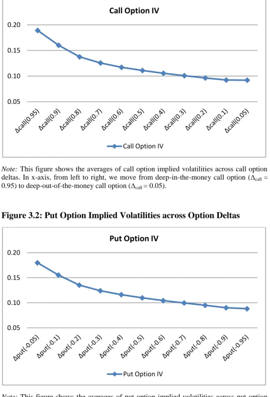
from out-of-the-money to in-the-money. Figure 3.1 and 3.2 show the averages of call

option and put option implied volatilities across deltas respectively for the whole data

(35)

25

Figure 3.1: Call Option Implied Volatilities across Option Deltas

Note: This figure shows the averages of call option implied volatilities across call option

deltas. In x-axis, from left to right, we move from deep-in-the-money call option (∆call =

0.95) to deep-out-of-the-money call option (∆call = 0.05).

Figure 3.2: Put Option Implied Volatilities across Option Deltas

Note: This figure shows the averages of put option implied volatilities across put option

deltas. In x-axis, from left to right, we move from deep-out-of-the-money put option (∆put

= -0.05) to deep-in-the-money put option (∆put = -0.95).

0.05 0.10 0.15 0.20 Call Option IV Call Option IV 0.05 0.10 0.15 0.20 Put Option IV Put Option IV

(36)

26

I define implied volatility smirk slope as the difference between put option

implied volatility of specific moneyness and at-the-money call option implied

volatility which is consistent with the recent literature. By using six different put

options with respect to their deltas, I calculate six different slope levels as follows;

S0 ν (-0.5) – ν (0.5) S1 ν (-0.4) – ν (0.5) S2 ν (-0.3) – ν (0.5) S3 ν (-0.2) – ν (0.5) S4 ν (-0.1) – ν (0.5) S5 ν (-0.05) – ν (0.5)

The slopes are calculated starting with the at-the-money put options and moving

to deep-out-of-the-money put options from S0 to S5. As reported in earlier studies, I

expect the slope to increase from S0 to S5. Because, put option implied volatility

(37)

27

option. Appendix A and B provides the descriptive statistics and time series plots for

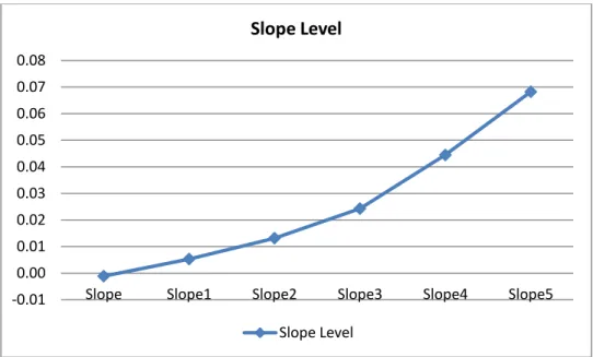
each slope levels respectively. Figure 3.3 depicts the averages of the slopes for the

whole data period.

Figure 3.3: Implied Volatility Smirk Slope Levels

Note: This figure shows the pattern of slope levels across different slope definitions. As it

can be observed from the figure, slope level increases when we move from at-the-money put option to deep-out-of-the-money put option.

3.1.3 Data Screening

In this section I perform diagnostic tests on the 5 minute intraday data. In high

frequency analysis, it is important to examine the data for intraday patterns and to -0.01 0.00 0.01 0.02 0.03 0.04 0.05 0.06 0.07 0.08

Slope Slope1 Slope2 Slope3 Slope4 Slope5

Slope Level

(38)

28

properly correct the data for further analysis. In addition to intraday patterns,

stationarity conditions are also checked. As, non-stationarity can cause spurious

regressions with erroneous estimates and results.

For intraday pattern diagnosis, I calculate the average of each variable for each 5

minute time interval in 250 trading day. Just for change in index level I use the

absolute values when calculating average of time intervals in order not the change in

prices cancel each other. Then I plot the averages across the time intervals whether

any pattern exist or not. Figures 3.4a to 3.4f give the plots of average values of time

intervals for slope measures.

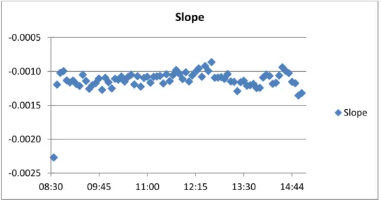
Figure 3.4a: Intraday Pattern of S0

Note: This figure shows the intraday pattern of S0. I take the average of whole period for

each time interval. -0.0025 -0.0020 -0.0015 -0.0010 -0.0005 08:30 09:45 11:00 12:15 13:30 14:44 Slope Slope

(39)

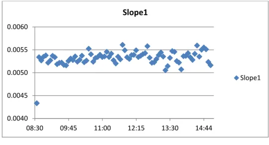
29 Figure 3.4b: Intraday Pattern of S1

each time interval.

Figure 3.4c: Intraday Pattern of S2

each time interval. 0.0040 0.0045 0.0050 0.0055 0.0060 08:30 09:45 11:00 12:15 13:30 14:44 Slope1 Slope1 0.0120 0.0125 0.0130 0.0135 0.0140 08:30 09:45 11:00 12:15 13:30 14:44 Slope2 Slope2

(40)

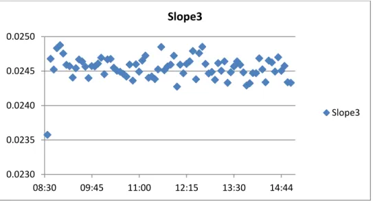
30 Figure 3.4d: Intraday Pattern of S3

each time interval.

Figure 3.4e: Intraday Pattern of S4

each time interval. 0.0230 0.0235 0.0240 0.0245 0.0250 08:30 09:45 11:00 12:15 13:30 14:44 Slope3 Slope3 0.044 0.0445 0.045 0.0455 0.046 08:30 09:45 11:00 12:15 13:30 14:44 Slope4 Slope4

(41)

31 Figure 3.4f: Intraday Pattern of S5

each time interval.

As it can be seen from the figures, other than the opening time values, there

seems no significant intraday pattern or outlier. Although the opening time value

seems not problematic for S4 and S5, for the remaining slope measures it is about 6

standard deviations away from the mean of time intervals. Therefore, I throw away

opening time from analysis in order to get reliable estimates.

For index returns, I observe from the data that there occur significant jumps

from previous day’s closing price to next day’s opening price. Similar to slope

measures, I throw away the opening time of index return. From Figure 4g, in addition

to opening time problem, index returns exhibit the intraday u-shaped pattern. In order 0.067 0.0675 0.068 0.0685 0.069 08:30 09:45 11:00 12:15 13:30 14:44 Slope5 Slope5

(42)

32

to get reliable estimates, I apply Flexible Fourier Form (FFF) transformation to

intraday index returns. Following Andersen and Bollerslev (1997, 1998), the following

decomposition of the intraday returns is considered;

where , , Zt,n is the

i.id. mean zero unit variance innovation term, N refers to the number of return

intervals per day. By squaring and taking logs of both sides, the equation becomes;

2 ln

The seasonal pattern is estimated by using ordinary least square estimation

(OLS);

where N1 = (N + 1) / 2 and N2 = (N + 1)(N + 2) / 6 are normalizing constants. Based on

(43)

33

the shape of the periodic pattern in the market to also depend on the overall level of

the volatility. Also the combination of trigonometric functions and polynomial terms

are likely to result in better approximation properties when estimating regularly

recurring cycles. The intraday seasonal pattern is then determined by using fitted

values of OLS;

Periodically filtered series is obtained by dividing the original series by the

estimated seasonal pattern.

(44)

34

Figure 3.4g: Intraday Pattern of Index Return

Note: This figure shows the intraday pattern of absolute value of Index returns and the intraday

pattern of deseasonalized of absolute value of Index returns. I take the average of whole period for each time interval.

As it can be seen from the figure 3.4g, the Flexible Fourier Form transformation

makes the intraday pattern more smoother. The FFF representation provides an

excellent overall characterization of the intraday periodicity. In the following sections

of this study, I am going to use this transformed series.

Another problem that leads to unreliable estimates is the non-stationarity of

variables. Thus, I perform some unit root test to each of the variable to test for

stationarity. The first test that I perform is augmented Dickey-Fuller (ADF) test (Said

and Dickey, 1984). The ADF test tests the null hypothesis that a time series is I(1) 0.0001 0.0003 0.0005 0.0007 0.0009 08:39 09:54 11:09 12:24 13:39 14:54 Abs(LogRet) Abs(FilteredLogRet)

(45)

35

against the alternative that it is I(0), assuming that the dynamics in the data have an

ARMA structure. Specification of the lag length is the most important practical issue

for the implementation of ADF. When choosing lag length, I follow the data

dependent lag length selection procedure of Ng and Perron (1995) that results in

stables size of the test and minimal power loss. In addition ADF test, I also perform

modified efficient Philips Perron (MPP) test (Ng and Perron, 2001). Compared to

standard PP test, this test does not exhibit the severe size distortions for errors with

large negative MA or AR roots, and they can have substantially higher power than the

PP test. Table 3.1 gives the statistics of these tests for each variable.

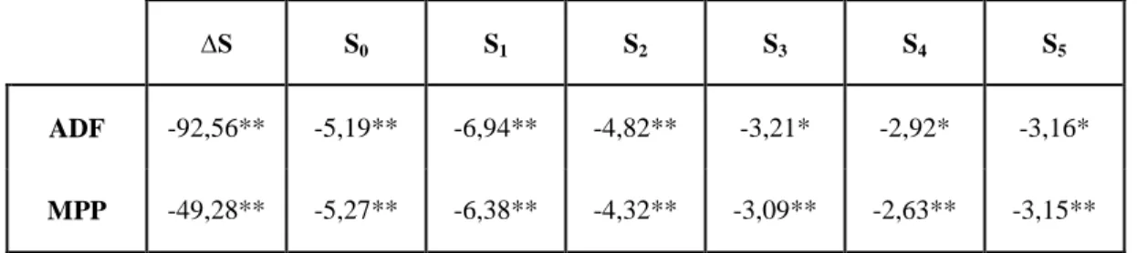
Table 3.1: Unit Root Tests of Variables

∆S S0 S1 S2 S3 S4 S5

ADF -92,56** -5,19** -6,94** -4,82** -3,21* -2,92* -3,16*

MPP -49,28** -5,27** -6,38** -4,32** -3,09** -2,63** -3,15**

Note: Table gives the t-values of the test statistics. ADF denotes the augmented Dickey-Fuller test;

MPP denotes the modified efficient Philips-Perron test. (**) and (*) corresponds the 1% and 5% significance levels respectively.

From the unit root tests that I conduct, all of the variables seem stationary. Both

ADF and MPP test give similar results. Almost all of the test statistics are significant

at 1% significance level. Therefore, I strongly reject the hypothesis of there is unit root

(46)

36 3.2 Methodology

3.2.1 Univariate ARIMA and ARFIMA models

I use a number of univariate time series models to examine whether the implied

volatility smirks can be predicted. The reason for using competing models is the

question of predictability is a joint hypothesis test of the forecasting model used.

The autocorrelations of all slope measures are characterized by a slow decay.

Figures 4.5a to 4.5f depict the ACF plots of slope variables. As it can be observed

from the plots, all slope measures have significant persistency. The highly persistent

autocorrelation behavior of the data suggests that its dynamics may be represented by

a long memory process. In empirical settings, when a time series is highly persistent or

appears to be non-stationary, researchers difference the time series once to achieve

stationary. However, for some highly persistent economic and financial time series, it

appears that an integer difference may be too much, which is indicated by the fact that

the spectral density vanishes at zero frequency for the differenced time series.

Therefore, instead of integer differencing, fractional differencing is suitable for long

(47)

37 Figure 4.5a: ACF Plot of S0

Lag A C F 0 50 100 150 200 0. 0 0. 2 0. 4 0. 6 0. 8 1. 0 Acf of Sl ope

Note: This figure shows the ACF plot of S0 up to 200 lags.

Figure 4.5b: ACF Plot of S1

Lag A C F 0 50 100 150 200 0. 0 0. 2 0. 4 0. 6 0. 8 1. 0 Acf o f Sl o p e 1

(48)

38 Figure 4.5c: ACF Plot of S2

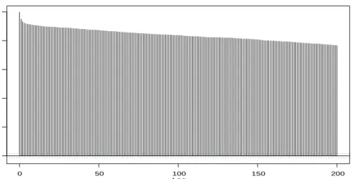
Figure 4.5d: ACF Plot of S3

Lag AC F 0 50 100 150 200 0. 0 0. 2 0. 4 0. 6 0. 8 1. 0 Acf of Slope2 Lag AC F 0 50 100 150 200 0. 0 0. 2 0. 4 0. 6 0. 8 1. 0 Acf of Slope3

(49)

39 Figure 4.5e: ACF Plot of S4

Figure 4.5f: ACF Plot of S5

Lag AC F 0 50 100 150 200 0. 0 0. 2 0. 4 0. 6 0. 8 1. 0 Acf of Slope4 Lag AC F 0 50 100 150 200 0. 0 0. 2 0. 4 0. 6 0. 8 1. 0 Acf of Slope5

(50)

40

Granger and Joyeux (1980) and Hosking (1981) introduced a flexible class of

long memory processes; called autoregressive fractionally integrated moving average

models (ARFIMA)12. The ARFIMA (p, d, q) model for a process yt is defined by

(L)(1 - L)d

(yt - μ) = θ(L)εt

where d denotes the non-integer order of fractional integration, (1 - L)d is the fractional difference operator, (L) and θ(L) denote the autoregressive component and moving average component respectively; and μ denotes the expected value of yt

processes and and εt is a Gaussian white noise process with zero mean and variance ξ2.

In the case where |d| < 0.5, the ARFIMA (p, d, q) process is invertible and

second-order stationary. In particular, if 0 < d < 0.5 (-0.5 < d < 0) the process is said to exhibit

long-memory (antipersistent) in the sense that the sum of the autocorrelation functions

diverges to infinity (a constant). The spectral density function of an ARFIMA(p, d, q)

model is given by;

12_{For an excellent survey of long memory processes, including applications to financial data, see}

(51)

41

Gallant et al. (1999) show that the sum of a particular AR(1) models is an

alternative to long memory that is also able to explain the highly persistent

characteristics of volatility. With the same motivation, ARIMA (p, d, q) model is also

employed to take into account the possible presence of short memory characteristics.

The ARIMA (p, d, q) model for a process yt is given by

(L)(1 - L)d

(yt - μ) = θ(L)εt

where d is an integer now that dictates the order of integration needed to

produce a stationary and invertible process (in our case d = 0), L is the lag operator, (L) = 1 + 1 L + … + p Lp is the autoregressive polynomial, θ(L) = 1 + θ1 L + … +

θq Lq is the moving average polynomial, μ is the mean of yt process and εt is a

Gaussian white noise process with zero mean and variance ξ2

. The spectral density

function of the general ARMA (p, q) model is given by;

(52)

42

3.2.2 Distributed Lag Models for Information Flows

I carry out a Granger causality test in order to observe lead-lag relationship

between variables. The first step in the causality test procedure involves identification

of the individual univariate time series using autoregressive integrated moving average

(ARIMA) models to generate filtered series. In this test, each variable is regressed on

a constant and p of its own lags as well as on p lags of other variable by the following

vector autoregression VAR(p) model:

Rt = 0 + (i). Rt-i + t

where Rt is the (2 x 1) vector of S&P 500 Index returns and the slope measure,

0 is the (2 x 1) vector of constants and (i) is the (2 x 2) matrix of autoregressive

slope coefficients for lag i.

However this VAR model does not contain contemporaneous variables. We

need these variables in order to test whether information flows immediately one

(53)

43

Rt = -1 + (i). St-i + t

where Rt denotes the filtered time series of index returns, and St is the option

volatility smile slope series of interest. Lags of slope measures are denoted by subscripts t - 1, t - 2,..., the coefficients with subscript -1 are constant terms, t is the

disturbance term.

Given the filtering of our series, the constant term would be expected to pick up

any remaining market frictions. The other terms pick up the interactions between the

markets. If these interactions occur simultaneously, we would expect 0 to be

significant, with none of the lag coefficients being significant. If, instead, market

linkages take some time, then these lag effects would be identified by significance of

the coefficients on the lagged slope series.

Formally, the null hypothesis that the markets are in a separating equilibrium

and thus the option implied volatility slope series does not have predictive power for

index returns. An extension of this hypothesis is to investigate the timing and direction

of the predictive power of the joint series. This can be addressed by examining the

behavior of the individual lag coefficients. In particular, the null hypothesis that the

(54)

44

Hypothesis: i = 0, individually for i = 1, 2, ……. , p

This hypothesis can be tested by simple t-tests of the significance of the

(55)

45

CHAPTER 4 ANALYSIS

The aim of this study is to model the time series behavior of the implied

volatility smirk slope levels and also to show the relationship between these slope

levels and index returns. For these purposes two approaches, univariate analysis and

time series regression analysis, are employed respectively.

The first part of this section presents the results of univariate analyses. In the

(56)

46 4.1 Univariate Analysis

4.1.1 In-Sample Evidence

In this section, I estimate the parameters of ARMA (p, q) and ARFIMA (p, d, q)

models for the in-sample period. My in-sample period covers the period of January 3,

2006 to July 3, 2006. After the estimation of the models, I assess the out-of-sample

performance of each model specification. The out-of-sample exercise is performed

from July 4, 2006 to December 29, 2006.

When estimating the parameters of ARFIMA (p, d, q) models, I perform

maximum likelihood estimation in the frequency domain by using the Whittle

approximation of the Gaussian log-likelihood. The log-likelihood function in the

frequency domain for a Gaussian process is as follows;

(57)

47

where f is the theoretical spectral density of the process. The spectral density f

at frequency is given by the spectral density function of ARFIMA model, while is the value of the periodogram at frequency

Similar to estimation of ARFIMA (p, d, q), I perform conditional maximum

likelihood estimation when estimating the parameters of ARMA (p, q) model. The

conditional likelihood treats the p initial values of the series as fixed and often sets the

q initial values of the error terms to zero. The autoregressive and moving average orders are chosen according to Bayesian Information Criterion (BIC).

Table 4.1 presents the maximum likelihood estimates and their standard errors

of the parameters of two competing models for 5-minute slope series. The values in

white blocks are the standard errors of the parameters.

As table 4.1 suggests, for the ARFIMA (2, d, 1) model, the fractional integration

parameter is highly significant for all of the slope levels. It ranges from -0.26 to -0.11.

The fractional integration parameter is negative and also its absolute value is lower

than 0.5 for all slope measures. Therefore, ARFIMA (2, d, 1) process is invertible and

(58)

48

that, instead of long memory process, the slope series exhibit antipersistent process. It

means that the sum of the autocorrelation functions diverges to a constant.

Autoregressive and moving-average parameters of the ARFIMA (2, d, 1) model

is also highly significant for all of the slope measures. The sum of the two AR

parameters is lower than 1 for each measure. The value of the moving-average

parameter ranges from 0.72 to 0.84 and all of them are highly statistically significant.

In addition to ARFIMA (2, d, 1), table 4.1 gives ARMA (2, 1) maximum

likelihood estimates and their corresponding standard errors. For all slope levels the

estimates for the ARMA (2, 1) model can be interpreted as the sum of persistent and

(59)

49

Table 4.1: Maximum likelihood estimation of ARMA and ARFIMA models for implied volatility smirk slope levels

Slope Slope1 Slope2 Slope3 Slope4 Slope5

Model 1 _{(2, 0, 1)} Model 2 _{(2, d, 1)} Model 1 _{(2, 0, 1)} Model 2 _{(2, d, 1)} Model 1 _{(2, 0, 1)} Model 2 _{(2, d, 1)} Model 1 _{(2, 0, 1)} Model 2 _{(2, d, 1)} Model 1 _{(2, 0, 1)} Model 2 _{(2, d, 1)} Model 1 _{(2, 0, 1)} Model 2 _{(2, d, 1)}

d -0.2419 -0.2585 -0.2588 -0.1366 -0.1165 -0.1081 0.0221 0.0224 0.0194 0.0161 0.0140 0.0117 AR(1) 14.335 15.884 14.327 16.053 13.929 15.516 13.676 14.395 12.975 13.423 11.359 11.844 0.0091 0.0222 0.0084 0.0222 0.0086 0.0205 0.0095 0.0187 0.0104 0.0176 0.0091 0.0166 AR(2) -0.4349 -0.5889 -0.4331 -0.6057 -0.3930 -0.5518 -0.3676 -0.4398 -0.2975 -0.3426 -0.1359 -0.1849 0.0090 0.0221 0.0083 0.0221 0.0086 0.0205 0.0095 0.0186 0.0104 0.0175 0.0091 0.0165 MA(1) 0.8830 0.8096 0.9093 0.8394 0.8953 0.8062 0.8545 0.7946 0.8051 0.7366 0.8347 0.7200 0.0049 0.0045 0.0039 0.0042 0.0042 0.0046 0.0053 0.0048 0.0064 0.0058 0.0051 0.0065

Note: This table gives the estimates of the ARMA (2,1) and ARFIMA (2, d, 1) models for the 6 different 5-minute implied volatility smirk

slope levels, from January 3, 2006 to July 3, 2006 (In-sample period). AR(1) and AR(2) are first and second order autoregressive parameters, MA(1) is the first order moving-average parameter, and "d " is the fractional integration. The estimates of the parameters are obtained by maximum likelihood estimation. The values in white blocks are the standard errors of the estimated parameters.

(60)

50

The estimates of the autoregressive and moving-average parameters of ARMA

(2, 1) model is almost similar to estimates of ARFIMA (2, d, 1) model. The sum of the

two autoregressive estimates is lower than 1 and the moving-average component

ranges from 0.81 to 0.91. All of the estimates for each slope measure are highly

statistically significant.

4.1.2 Out-of-sample forecasting performance

I assess the out-of-sample performance of ARMA (2, 1) and ARFIMA (2, d, 1)

models that are estimated in the previous part. The out-of-sample exercise is

performed from July 4, 2006 to December 29, 2006. I form the 1-day ahead and 3-day

ahead point forecasts for each of slope measure.

I use two alternative metrics to assess the statistical significance of the

out-of-sample point forecasts obtained. The first metric is the mean squared prediction error

(MSE), calculated as the average squared deviations of the actual slope levels from the

model based forecast, averaged over the number of observations. The second metric is

(61)

51

differences between the actual slope levels and the model based forecast, averaged

over the number of observations.

Table 4.2 and 4.3 gives the results of forecast metrics of 1-day ahead and 3-day

ahead predictions respectively for each of the slope measures.

Table 4.2: 1-day ahead forecast performances of ARMA and ARFIMA models

1 Day Ahead

MSE-ARMA MSE-ARFIMA MAE-ARMA MAE-ARFIMA

Slope 0.000004 0.000007 0.0016 0.0021 Slope1 0.000005 0.000021 0.0018 0.0034 Slope2 0.000006 0.000014 0.0019 0.0029 Slope3 0.000009 0.000029 0.0023 0.0039 Slope4 0.000017 0.000052 0.0032 0.0050 Slope5 0.000041 0.000087 0.0049 0.0064

Note: This table gives the out of sample (from July 3, 2006 to December 29, 2006) one day forecast

evaluation statistics of ARMA and ARFIMA models for each of the slope levels. MSE corresponds to mean squared error, and MAE corresponds to mean absolute error. Interval between forecasts equal to one day in order not to create overlapping data problem.

(62)

52

Table 4.3: 3-day ahead forecast performances of ARMA and ARFIMA models

3 Day Ahead

MSE-ARMA MSE-ARFIMA MAE-ARMA MAE-ARFIMA

Note: This table gives the out of sample (from July 3, 2006 to December 29, 2006) three day

forecast evaluation statistics of ARMA and ARFIMA models for each of the slope levels. MSE corresponds to mean squared error, and MAE corresponds to mean absolute error. Interval between forecasts equal to three day in order not to create overlapping data problem.

As Table 4.2 suggests, in 1-day forecasts, ARMA performs better than ARFIMA

model both in terms of MSE and MAE for all of the slope measures. Similarly, in

3-day forecasts, ARMA model is still a bit better than the ARFIMA model, but the

difference seems smaller compared to 1-day ahead forecasts. As a result, I can say that

ARMA model has smaller prediction errors compared to ARFIMA model for all slope

(63)

53

Although, there seems differences in the statistics of forecast metrics among

competing models, these differences should have statistical meaning. For this reason, I

use Diebold-Mariano (DM) (1995) statistics to determine if one model's forecast is

more accurate than another's. The null hypothesis of this procedure is the two

competing models have equal forecasting accuracy. Diebold and Mariano show that

under the null hypothesis of equal predictive accuracy the DM statistic is

asymptotically distributed N(0, 1). The Diebold-Mariano test statistic is as follows;

where

is the average loss differential, and is a consistent estimate of the long-run asymptotic variance of .

Table 4.4 gives the result of Diebold-Mariano test statistics of 1-day and 3-day

evaluation periods for each of the slope measures. The results indicate that all of the

(64)

54

null hypothesis of two competing models have equal predictive accuracy. There is no

statistically significant differences in terms of predictive accuracy among ARMA (2,1)

and ARFIMA (2, d, 1) models.

Table 4.4: DM Statistics of 1-day ahead and 3-day ahead forecasts

1 Day Ahead 3 Day Ahead

DM-MSE DM-MAE DM-MSE DM-MAE

Note: This table gives the results of Diebold-Mariano (DM) statistics for 1-day and 3-day ahead