A LEARNING-BASED SCHEDULING SYSTEM WITH
CONTINUOUS CONTROL AND UPDATE STRUCTURE
A THESIS
SUBMITTED TO THE DEPARTMENT OF INDUSTRIAL ENGINEERING AND THE INSTITUTE OF ENGINEERING AND SCIENCE
OF BILKENT UNIVERSITY
IN PARTIAL FULFILLMENT OF THE REQUIREMENTS FOR THE DEGREE OF
MASTER OF SCIENCE
By Gökhan Metan
I certify that I have read this thesis and that in my opinion it is fully adequate, in scope and in quality, as a thesis for the degree of Master of Science.
Prof. Dr. İhsan Sabuncuoğlu (Supervisor)
I certify that I have read this thesis and that in my opinion it is fully adequate, in scope and in quality, as a thesis for the degree of Master of Science.
Prof. Dr. Erdal Erel
I certify that I have read this thesis and that in my opinion it is fully adequate, in scope and in quality, as a thesis for the degree of Master of Science.
Asst. Prof. Dr. Mehmet Taner
Approved for the Institute of Engineering and Sciences:
Prof. Dr. Mehmet Baray
ABSTRACT
A LEARNING-BASED SCHEDULING SYSTEM WITH
CONTINUOUS CONTROL AND UPDATE STRUCTURE
Gökhan Metan
M.S. in Industrial Engineering Supervisor: Prof. Dr. İhsan Sabuncuoğlu
January, 2005
In today’s highly competitive business environment, the product varieties of firms tend to increase and the demand patterns of commodities change rapidly. Especially for high tech industries, the product life cycles become very short and the customer demand can change drastically due to the introduction of new technologies in the market (i.e., introduction by the competitors). These factors increase the need for more efficient scheduling strategies. In this thesis, a learning-based scheduling system for a classical job shop problem with the average tardiness objective is developed. The system learns on the manufacturing environment by constructing a learning tree and selects a dispatching rule from the tree for each scheduling period to schedule the operations. The system also utilizes the process control charts to monitor the performance of the learning tree and the tree as well as the control charts is updated when necessary. Therefore, the system adapts itself for the changes in the manufacturing environment and survives in time. Also, extensive simulation experiments are performed for the system parameters such as monitoring (MPL) and scheduling period lengths (SPL). Our results indicate that the system performance is significantly affected by the parameters (i.e., MPL and SPL). Moreover, simulation results show that the performance of the proposed system is considerably better than the simulation-based single-pass and multi-pass scheduling algorithms available in the literature.
Keywords: Scheduling, Machine Learning, Data Mining, Control Charts, Job Shop Scheduling, AI, Dispatching Rules.
ÖZET
SÜREKLİ KONTROL VE GÜNCELLEŞTİRME YAPILI
ÖĞRENME TEMELLİ ÇİZELGELEME SİSTEMİ
Gökhan Metan
Endüstri Mühendisliği, Yüksek Lisans Tez Yöneticisi: Prof. Dr. İhsan Sabuncuoğlu
Ocak, 2005
Günümüzün rekabetçi iş dünyasında firmaların ürün çeşitleri artmakta ve malların talep düzeni hızlı bir şekilde değişmektedir. Özellikle yüksek teknoloji endüstrilerinde yeni teknolojilerin pazara tanıtımlarıyla ürün ömür çevrimleri kısalmakta ve müşteri talebi şiddetli şekilde değişmektedir. Bu etmenler verimli çizelgeleme gengüdümlerine olan ihtiyacı artırmaktadır. Bu tezde, geleneksel atelye problemine ortalama gecikme amacına yönelik öğrenme temelli çizelgeleme sistemi geliştirilmiştir. Önerilen sistem öğrenme ağacı kurmak yoluyla üretim ortamı üzerinde öğrenmekte ve bu ağaçtan herbir çizelgeleme dönemi için dağıtım kuralı seçerek işlemleri çizelgelemektedir. Sistem aynı zamanda süreç denetim çizeneklerinden faydalanarak öğrenme ağacının başarımını gözetlemekte ve gerekli bulduğunda ağacı ve denetim çizeneklerini güncellemektedir. Bu sayede, önerilen sistem kendi kendini üretim ortamındaki değişikliklere uyarlamakta ve zaman içinde hayatta kalabilmektedir. Bunun yanı sıra, çizelgeleme dönem uzunluğu ve gözetleme dönem uzunlukları gibi sistem parametreleri üzerinde kapsamlı benzetim deneyleri gerçekleştirilmiştir. Sonuçların gösterdiğine göre bu parametreler sistem başarımını (ortalama gecikme) önemli şekilde etkilemektedir. Bundan başka, benzetim sonuçları önerilen sistemin başarımının benzetim-temelli tek-geçişli ve çok-geçişli çizelgeleme algoritmalarından daha iyi olduğunu göstermektedir.
Acknowledgement
I would like to express my deepest gratitude to my supervisor Prof. Dr. İhsan Sabuncuoğlu for his instructive comments in the supervision of the thesis and also for all the encouragement and trust during my graduate study.
I would like to express my special thanks and gratitude to Prof. Dr. Erdal Erel and Asst. Prof. Dr. Mehmet Taner for showing keen interest to the subject matter, for their remarks, recommendations and accepting to read and review the thesis.
I would like to express my deepest thanks to Kürşad Derinkuyu, Emrah Zarifoğlu, Ali Koç, M. Oğuz Atan, Halil Şekerci, Arda Alp and Mustafa R. Kılınç for all their encouragements and supports.
I would like to extend my sincere thanks to Orçun Ergün, Esra Büyüktahtakın and Banu Yüksel for their endless morale support and friendship during all my desperate times, makes me to face with all the troubles.
I would also like expressing my greatest thanks to Şermin Kamberli, Şengül Deveci and Uğur Deveci for being like my second family and showing all their supports. Finally, I would like to express my gratitude to my family and my wife for their love, understanding, suggestions and their endless support. I owe so much to my family and my wife. I love you both…
Contents
Abstract...iii Özet...iv Acknowledgement...vi Contents ...vii List of Figures... xList of Tables ...xii
1 Introduction... 1
2 Literature Review ... 5
3 Proposed System: Intelligent Scheduling with Machine Learning ... 14
3.1 Definitions ... 15 3.2 Proposed System... 16 3.3 Scheduling Strategy... 18 3.3.1 How-to-schedule... 18 3.3.2 When-to-schedule... 19 3.4 Data Structures... 23
3.4.1 Performance Data (Realized System Performance) ... 24
3.4.2 Instance Data ... 26
3.4.3 Realized Scheduling Period Data... 27
3.5 Proposed System - A Detailed Explanation ... 28
3.5.2 Simulation Module ... 29
3.5.3 Learning Module ... 29
3.5.4 On-line Controller ... 33
3.5.5 Process Controller ... 34
3.6 System Attributes for Job Shop Scheduling System ... 41
3.7 Dynamics of the Learning Algorithm ... 43
3.8 Summary... 49
4 Experimental Design and Computational Results ... 50
4.1 Motivation... 51
4.2 Setting Due Date Tightness Levels and Utilization Levels... 55
4.3 Setting Appropriate Scheduling Period Length (SPL) ... 56
4.4 The Effect of Monitoring Point (MP) and β-parameter Selection ... 65
4.5 The Selection of System Attributes ... 70
4.6 Job Shop Scheduling with a Static Learning Tree... 73
4.7 Job Shop Scheduling with Dynamic Learning Structure ... 78
4.8 Summary... 92
5 Conclusion and Future Research Directions... 94
5.1 Contributions ... 94 5.2 Future Research ... 97 Bibliography ... 99 Appendix... 101 A1 Appendix A... 101 A2 Appendix B ... 103
A3 Appendix C ... 113
A4 Appendix D... 120
A5 Appendix E ... 126
List of Figures
3.1 Proposed system – general structure... 17
3.2 Representation of rule selection symptoms. ... 21
3.3 Rule selection symptoms... 22
3.4 Types of performance data... 25
3.5 Instance data representation. ... 26
3.6 Realized scheduling period data... 28
3.7 Database of the proposed system. ... 30
3.8 Simulation module... 31
3.9 Learning module... 32
3.10 On-line controller... 35
3.11 Process controller module and its relationships with other modules. ... 37
3.12 Plotted data in the X chart. ... 38
3.13 Construction of the learning tree: first step... 47
3.14 Construction of the learning tree: second step... 48
3.15 Construction of the learning tree: third step. ... 48
3.16 Final learning tree... 48
4.1 Performance measures... 53
4.2 80% utilization, loose due dates with CDR set {MOD, SPT, MDD, ODD}. ... 58
4.3 90% utilization, loose due dates with CDR set {MOD, SPT, MDD, ODD}. ... 59
4.4 80% utilization, tight due dates with CDR set {MOD, SPT, MDD,
ODD}. ... 60
4.5 90% utilization, tight due dates with CDR set {MOD, SPT, MDD, ODD}. ... 61
4.6 80% utilization, tight due dates with CDR set {SPT, MDD, ODD}. ... 63
4.7 90% utilization, tight due dates with CDR set {SPT, MDD, ODD}. ... 64
4.8 BestPerf for various MPL-β combinations when system utilization is 80% ... 67
4.9 Comparison of best MPL-β pairs for 80% utilization. ... 68
4.10 BestPerf for various MPL-β combinations when system utilization is 90% ... 69
4.11 Comparison of best MPL-β pairs for 90% utilization... 70
4.12 X chart... 89
List of Tables
3.1 Parameters of how-to-schedule. ... 19
3.2 New rule selection symptoms. ... 20
3.3 Update only learning tree rules.. ... 40
3.4 Update both the learning tree and the process control charts rules... 41
3.5 Artificial training data set... 45
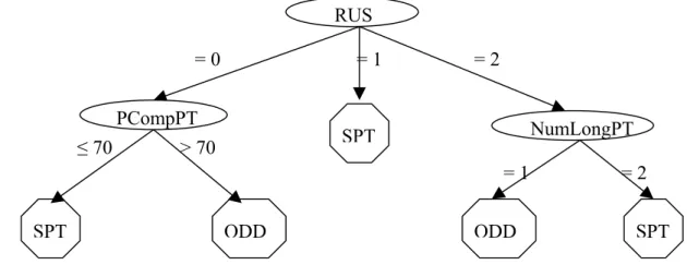
3.6 Subset of initial data set for branch RUS=0.. ... 48
4.1 Simulation results for flow allowances... 56
4.2 Experimental design of scheduling period length.. ... 56
4.3 Parameter values considered for further experimentation... 63
4.4 Experimental design of monitoring period length and β-parameter... 66
4.5 Experimental conditions for generated data sets.. ... 73
4.6 Summary of the experimental results on the attribute set selection... 73
4.7 Experimental design of scheduling with a static learning tree... 74
4.8 Summary of performance values for the rule set {SPT, MDD, ODD}..76
4.9 Summary of performance values for the rule set {SPT, MDD, ODD , MOD}.. ... 76
4.10 Average dispatching rule usage percentages.. ... 77
4.11 Experimental design of scheduling with dynamic learning structure.... 79
4.12 Summary of the experimental results for DR set {MDD, ODD, SPT}..82
4.13 Summary of the experimental results for DR set {MDD, ODD, SPT,
MOD}.. ... 83
4.14 Summary of the experimental results for DR set {MDD, ODD, SPT} (Percentage of deviation from the best).. ... 85
4.15 Summary of the experimental results for DR set {MDD, ODD, SPT, MOD} (Percentage of deviation from the best)... 86
C.1 80% utilization, tight due dates replication mean tardiness values (DR set SPT, MDD, MOD, ODD)... 114
C.2 90% utilization, tight due dates replication mean tardiness values. (DR set SPT, MDD, MOD, ODD)... 115
C.3 80% utilization, loose due dates replication mean tardiness values. (DR set SPT, MDD, MOD, ODD)... 116
C.4 90% utilization, loose due dates replication mean tardiness values. (DR set SPT, MDD, MOD, ODD)... 117
C.5 80% utilization, tight due dates replication mean tardiness values. (DR set SPT, MDD, ODD). ... 118
C.6 90% utilization, tight due dates replication mean tardiness values. (DR set SPT, MDD, ODD). ... 119
D.1 80% utilization, for MPL = 250 replication mean tardiness values... 121
D.2 80% utilization, for MPL = 500 replication mean tardiness values... 122
D.3 90% utilization, for MPL = 500 replication mean tardiness values... 123
D.4 90% utilization, for MPL = 2500 replication mean tardiness values.... 124
E.1 80% utilization, MPL = 250, β = 0.2, DR set {MDD, ODD, SPT}...127
E.2 80% utilization, MPL = 500, β = 1, DR set {MDD, ODD, SPT}...127
E.3 80% utilization, MPL = 1000, β = -, DR set {MDD, ODD, SPT}...127
E.4 90% utilization, MPL = 500, β = 0.2, DR set {MDD, ODD, SPT}...128
E.5 90% utilization, MPL = 2500, β = 1, DR set {MDD, ODD, SPT}...128
E.6 90% utilization, MPL = 7500, β = 1, DR set {MDD, ODD, SPT}...128
E.7 80% utilization, MPL = 250, β = 0.2, DR set {MOD, MDD, ODD, SPT}... 129
E.8 80% utilization, MPL = 500, β = 1, DR set {MOD, MDD, ODD, SPT}... 129
E.9 80% utilization, MPL = 1000, β = -, DR set {MOD, MDD, ODD, SPT}... 129
E.10 90% utilization, MPL = 500, β = 0.2, DR set {MOD, MDD, ODD, SPT}... 130
E.11 90% utilization, MPL = 2500, β = 1, DR set {MOD, MDD, ODD, SPT}... 130
E.12 90% utilization, MPL = 7500, β = 1, DR set {MOD, MDD, ODD, SPT}... 130
E.13 80% utilization, MPL = 250, β = 0.2, DR set {MDD, ODD, SPT}...131
E.14 80% utilization, MPL = 500, β = 1, DR set {MDD, ODD, SPT}...132
E.15 80% utilization, MPL = 1000, β = -, DR set {MDD, ODD, SPT}...133
E.17 90% utilization, MPL = 2500, β = 1, DR set {MDD, ODD, SPT}...135 E.18 90% utilization, MPL = 7500, β = 1, DR set {MDD, ODD, SPT}...136 F.1 Plotted data in the charts. ... 138 F.2 Number of updates for the learning tree and the charts for DR set {MOD, MDD, ODD, SPT}. ... 140 F.3 Number of updates for the learning tree and the charts for DR set {MDD, ODD, SPT}... 140
Chapter 1
Introduction
In today’s highly competitive business environment, customer satisfaction plays the key role for the success of any firm. Customers not only care about the cost of a product, but they also give special importance to the quality of the products and the reliability of the manufacturers in terms of meeting their agreements such as the promised due dates. Moreover, the product variety of a firm tends to increase due to the demand for highly customized goods, which in turn increases the complexity of operating a manufacturing system. In addition to these, the demand patterns of commodities may also change too rapidly. Especially for high tech industries, the product life cycles become very short and the customer demand can change drastically due to the introduction of new technologies in the market (i.e., introduction by the competitors). These factors increase the need for more efficient manufacturing strategies and approaches.
One of the key elements for the success of any manufacturing firm is efficient scheduling of its limited resources. However, even for a small sized company with a few number of equipments, it can become a very difficult problem to deal with.
In addition to this, scheduling problems should be solved frequently since it is the lowest level tactical decision for a firm. Therefore, development of efficient scheduling algorithms is vitally important and there is a vast amount of literature on this issue.
When the scheduling problem is stochastic and dynamic (i.e., the jobs arrive dynamically to the system and the arrival and processing times are stochastic) in nature, scheduling via the dispatching rules are commonly preferred. Dispatching rules are myopic decision rules that schedule the jobs on the machines one at a time based on the simple calculations that utilizing the information such as processing times, due dates etc. There are many such rules defined in the literature and we can simply pick one of them and perform the scheduling activities. However, the problem with these dispatching rules is that none of them is superior to the others in every manufacturing condition. Therefore, the appropriate rule/s should be determined prior to the use. In addition to that, even if a particular dispatching rule is found to perform better for a specific manufacturing system, switching to the other rules in certain periods may result in additional benefits. For this reason, there are also some simulation-based scheduling approaches in the literature. For such studies see, for example, Kim and Kim (1994), Jeong and Kim (1998), Kutanoglu and Sabuncuoglu (2001). In this approach, simulation-based scheduling, a set of candidate dispatching rules are simulated for a planning period and the rule with the best performance value is used in that period. One of the shortcomings of this approach is that it requires too much computer time to simulate the performance of each candidate dispatching rule. Also, the procedure depends on the assumption that we know the probability distribution functions and the parameters of the processing and arrival times. However, this may not be the case if the demand patterns in the market and/or product
types change rapidly, which is the situation for high tech industries. Also, the processing times may change due to the machines’ depreciations in time. Hence, the simulation models constructed to evaluate the performance of the rules might become invalid after some time.
In this research, we consider the stochastic and dynamic job shop scheduling problem with the average tardiness (mean tardiness) objective and develop a system to select the right dispatching rule among a set of candidate rules. The proposed system utilizes the intelligent machine learning techniques from computer science (i.e., data mining) as well as the process control charts from the statistical quality control. The objective of our system is to learn about the characteristics of the manufacturing system by constructing a learning tree and then selecting a dispatching rule for a scheduling period from this tree on-line. Therefore, we eliminate the extensive simulation experiments that should be carried out before every scheduling period as it is in simulation-based scheduling approaches. Moreover, we use the control charts to monitor the actual performance of the learning tree. If these charts signal that the current learning tree begins to perform poorly, a new tree is constructed based on the recent information gathered from the manufacturing system. The reason for the current tree to have a poor performance might be a result of change in the demand patterns, processing time distributions and so on. Thus, by updating the current learning tree, we are targeting to capture these changes in the manufacturing system and select the right dispatching rules for the future periods. In this sense, the proposed system has the ability to survive in time. In other words, we propose a system that corrects itself whenever necessary (without an external manipulation) and continues to make the scheduling decisions (i.e., selecting the dispatching rules) as long as the manufacturing system exists.
In this study, we also address two important questions and conduct extensive experiments to answer them. One of these questions is “how frequently should we update the dispatching rule used in the manufacturing system?” This is a critical question since frequent selection of a new rule might result in system nervousness and, on the other hand, infrequent update of the rules most probably result in the loss of additional benefits that can be achieved by switching between the rules. The second question is “how frequently should we monitor the performance of the manufacturing system that operates under a rule and how should we decide to update or continue with this rule at these monitoring points?” Both of these questions are also important for the performance of our proposed system and experimented extensively.
In the next chapter, a review of the relevant literature is presented. In Chapter 3, we propose the intelligent scheduling system and discuss its key features in detail. Experimental designs and the results of these experiments are given in Chapter 4. Finally, in Chapter 5, we present the conclusion of this study along with the contributions and give future research directions.
CHAPTER 2
Literature Review
In the scheduling literature, there is a vast amount of studies that deal with various issues in scheduling. In this section, we will briefly review the relevant studies that employ iterative simulation and artificial intelligence (AI) concepts in manufacturing systems. In addition, we consider some studies related to process control charts as we use them as the tool in our research.
Wu and Wysk (1988) develop an expert system called multi-pass expert
control system (MPECS) for flexible manufacturing cells. This system takes
advantage of both expert system technology and discrete-event simulation. Simulation is employed as a prediction mechanism and evaluates the performance of the dispatching rules that are suggested by the expert system. Then, the dispatching rule that results the best performance value in simulation runs is used to schedule the jobs. This system also contains a simplified and restricted learning mechanism. This learning module uses training instances that relate the dispatching rules, the performance measures and the system characteristics together. By using this restricted learning mechanism, the system provides the user a learning aid, which collects information of the user interested factors (e.g., number of times a rule is selected, etc.)
to help the user learn from the system and modify the knowledge base if possible. In this sense, the system does not learn automatically by itself, but guides the user by providing significantly found information about the manufacturing system.
In another study by Wu and Wysk (1989), a simulation-based scheduling algorithm is proposed for flexible manufacturing system. In this research, a dispatching rule among a set of candidate rules is selected for each short period via simulation just before the implementation time occurs. The experiments on this candidate rule set are carried out by deterministic simulation and performance of each rule is estimated. Then the rule with the best performance estimate is used in that short period of time to schedule the operations. Since all the candidate dispatching rules are evaluated at each short scheduling period and the best performer is selected to be used in that interval, the proposed scheduling approach is termed as a multi-pass scheduling algorithm. Thus, in the long run, this process results in a combination of different dispatching rules. Their results show that the multi-pass scheduling algorithm performs better than the single-pass scheduling algorithm, which uses a single dispatching rule for the entire manufacturing period.
Another simulation-based scheduling study is due to Ishii and Talavage (1991). In this research, a transient-based real-time scheduling algorithm that selects a dispatching rule dynamically for a next short time period to react to changes of system state is proposed. In this study, as opposed to the work of Wu and Wysk (1989), the scheduling interval length, where each candidate dispatching rule is evaluated, is not held fixed and four different strategies are defined accordingly. In the first strategy, the simulation window (length of time used to evaluate the performance of candidate rules) is defined of equal length to the next scheduling interval as it is in the study of Wu and Wysk (1989). In the second strategy, simulation window is defined from the
current time to the time until all parts that exist in the system during the next scheduling interval depart from the system. For the third strategy, they define simulation window as from current time to the end of the entire manufacturing period. Finally, the last strategy assumes simulation window as the two consecutive scheduling intervals and selects the best rule for the first scheduling interval based on the performances measured at the end of the second scheduling interval. In this sense, the last strategy employs a single period look-ahead mechanism. It is reported in the paper that in most of the experiments strategy 4 results in better schedules than the other strategies as well as the single-pass scheduling algorithm.
The first study that applies machine learning techniques to the scheduling problems is the work of Shaw et. al. (1992). In this paper machine learning capabilities for an FMS scheduling problem is investigated. Their machine learning approach is used to select the best dispatching rule based on a number of manufacturing system characteristics (the overall system utilization, total buffer size and number of machines). This selected rule is then used to schedule the jobs on the machines, and the rule is never questioned again as long as the shop floor configuration is stable (e.g., number of machines in the facility doesn’t change). Therefore, the decision given in this study can be thought of as a strategic decision rather than a tactical one. Training examples are generated for different attribute-value combinations. These examples are supplied for the learning algorithm as a learning data set after being tested via simulation. After the learning algorithm processes the learning data, a learning tree is constructed. Whenever one or more of the system characteristics changes (takes a different value than its current value), the algorithm selects a new dispatching rule (DR) from the learning tree based on the new values of the attributes. It does not implement the new DR immediately, but rather it makes a
new decision about changing the current DR with this new one or not. This is because of the fact that some attribute changes may be temporary and changing the DR of the manufacturing system may be destructive when compared with the expected performance of the current DR. This decision is done in such a way that if the cumulative score (number of times a DR is favored to the others) of the new DR is greater than the cumulative score of the current DR multiplied by a smoothing factor, the new DR is selected for use. Otherwise, the system continues its operation with the current DR. Here, the smoothing factor is a decision variable between 0 and 1. Also, since smoothing factor is a decision variable, experimentation on this variable is performed with different attribute values for three smoothing factor values (0, 0.7 and 1) and another learning tree is constructed for the selection of this variable. In other words, the value of the smoothing factor is not a fixed value but its value is determined based on the system attributes from the second learning tree whenever a new DR is to be selected from the first learning tree. By using this machine learning strategy, Shaw et. al. test their algorithm on different FMS problems. The results indicate that the proposed approach outperforms the approach of using the single best DR from a set of candidate DRs in most of the cases.
In another series of studies by Tayanithi, Manivannan, and Banks (1993a, 1993b), an integrated scheduling and control system that combines simulation and knowledge-based concepts to perform an analysis of interruptions in the form of machine breakdowns and rush orders in a flexible manufacturing system is proposed. In this system, when a control decision cannot be obtained readily from the knowledge base, the alternative actions are evaluated by using the simulation mechanism.
Cho and Wysk (1993) propose a neural network based scheduling algorithm for FMS. Their system mainly composed of three parts: a preprocessor, a neural network and a multi-pass simulator. Preprocessor generates input based on the current workstation status and supplies it to the neural network. In turn, neural network produces a set of promising part dispatching strategies (i.e., dispatching rules) to guide the future scheduling activities. These strategies are then evaluated by the multi-pass simulator and the best strategy to use is determined. Then the selected strategy is used in the shop floor until a new rule update is required. The performance of the algorithm is compared with the single-pass strategies and found to be superior. Ishii and Talavage (1994) propose another simulation-based scheduling system for flexible manufacturing systems. In this research, they develop a mixed dispatching rule approach in which each individual machine in an FMS are allowed to have a different dispatching rule to perform the scheduling of jobs. It is assumed in the paper that the candidate dispatching rule set is predetermined and a search strategy to select the best combination from these candidate rules is employed. The effectiveness of the mixed dispatching rule approach is demonstrated by comparing the experimental results with the conventional approach, where a single dispatching rule is assigned for all machines in a system for a given scheduling interval.
One of the simulation-based studies for scheduling problems is due to Kim and Kim (1994), there is a candidate DR set and the rules in this set are evaluated at the beginning of each planning horizon by deterministic simulation. The best performer is then selected for use for that planning horizon. There are also monitoring points defined within the planning horizon and the actual performance of the DR (based on the stochastic simulation which represents the real life situation) is compared with the estimated one (from deterministic simulation at the beginning of
the planning horizon). If this difference exceeds the limit then a new DR is selected from the candidate set by the same procedure mentioned as above. In the follow up study, Jeong and Kim (1998) have extended the previous study. The dispatching rule selection approach is the same as the first study, where a set of candidate DRs are evaluated via simulation and the best one is selected for implementation. The major development in the later study is that the results from the different policies are defined for the question of “when to select a new rule?” Specifically, four different alternative policies are defined and compared in this study. The first policy is called as BEGIN and only selects a new DR at the beginning of each planning horizon. The second policy, MAJOR, considers selecting a new DR at the beginning of each planning horizon and at times within the planning horizon whenever a major breakdown of a machine occurs. The third one, MAJOR and PERIODIC (M&P), selects a new DR as MAJOR and additionally at monitoring points. And the final policy, so called ALL, selects a new DR at the beginning of each planning horizon, when a major breakdown occurs and a minor breakdown occurs, as well. The concept of major and minor breakdowns is a subjective issue and is defined by the authors in the paper with some parameters. The results of the experiments in the paper show that M&P and ALL perform best. Moreover, while evaluating the candidate DRs in the previous paper (Kim and Kim, 1994), authors used deterministic simulation. In this paper, authors also test the effect of using deterministic and stochastic simulations in the decision phase, that is, the point where we will select the best performing DR via simulation. Results show that the deterministic simulation, where the machine breakdowns are not considered, resulted in better selections of DRs.
Pierreval and Mebarki (1997) propose a system by which dispatching rules are selected dynamically. Their aim is to monitor the system continuously and select the
most suitable dispatching rule for each work-center to optimize the system performance. Actually, this research includes the following developments:
i- Allows for more than one performance criteria to be considered simultaneously (both primary and a secondary criteria are considered at the same time).
ii- Based on the specified performance criteria, dynamic selection of the DRs seems to be a good policy for the operating conditions and current shop
status.
iii- The capability of tracking the triggering events such as new job arrivals, resource availabilities etc.
In the light of these developments, a new heuristic technique called SFSR (shift from standard rules) is proposed. This mechanism has a default dispatching strategy based on the specified performance criteria. These default dispatching strategies are called as the ‘Standard Rules’. For example, R1, which is defined as the standard rule that applies whenever the primary objective is to reduce the mean flow time of jobs dictates the system the SPT rule and it is active if there is no anomalies (no triggering events) in the system. These standard rules are obtained from the literature based on their performances in the previous studies. There is also a second class of rules called as the ‘Diagnosis Rules’ that accounts for a major development. These rules work according to the symptoms detected in the system by continuously monitoring. A defined set of symptoms (new job arrivals, resource availability etc.) and their corresponding actions, so called the Diagnosis rules, aim at achieving better performances. However, the generation of these diagnosis rules is not based on a data mining approach but rather they are common sense rules that are based on experiences of humans. In this sense, this research cannot be classified as a machine
learning approach to scheduling problems, but it can be classified as a scheduling by using heuristic rules.
In another study by Kutanoglu and Sabuncuoglu (2001), an iterative simulation-based approach for the dynamic and stochastic job shops is proposed. In this study, at the beginning of each scheduling period, a set of DRs are tested via simulation under the current system conditions and the forecasts. The best performing DR is selected for the upcoming period and used until the next scheduling period. The rolling horizon technique is also employed in this study since the simulation runs are taken for longer time periods (more than one scheduling period).
Suwa and Fujii (2003) use a machine learning technique (data mining) for rule acquisition in a dynamic single machine scheduling problem. The training examples to the learning module are generated via simulation and then the learning tree is constructed. Afterwards, the learning tree is used for selecting the appropriate DR to schedule the jobs in a rolling horizon basis. The attributes used in this study to represent both the training examples and the conditions when selecting a new DR at the beginning of a new period are based on some performance measure differences between the current period and the last period. The learning tree is used forever after once it is constructed and no revision or critique of the existing rule base is performed.
A related study is the working paper by Huyet and Paris (2003). In this study, an evolutionary optimization method is used with machine learning in order to set the parameters of a Kanban system optimally. A population of 30 individuals is used in each generation of GA and at every three iterations, the machine learning is used to learn about the characteristics of promising solutions. Then a number of solutions generated randomly, but which have the characteristics found to be important by the
machine learning are embedded into the new generation and the process continues. In this research, machine learning mainly accelerates the convergence of the individuals and hence find the optimum (or near optimum) solutions more rapidly (approximately half of the iterations are found to be sufficient for the same level of convergence when compared with the GA used alone). This research is a good example to show the power of the machine learning approaches when they are employed effectively.
Another two related studies that show the applicability and usefulness of one of our tools in our proposed approach is the papers of Takahashi and Nakamura (1999, 2002). In these two papers, a reactive Kanban system is proposed, where the number of Kanban cards in the system is manipulated continuously as a response to the system parameter, the unstable changes in demand (both mean and the variance of the demand distribution is subject to change continuously). Since the demand distribution is not stable, the optimal parameters of the Kanban system (number of Kanban cards, Kanban container sizes etc.) change dynamically, as well. Therefore, appropriate actions should be taken in order to operate optimally or at least near optimally. In this paper, the Process Control Charts (EWMA) from quality control are employed in order to monitor the unstable changes in demand parameters. The demand distribution is assumed to be normally distributed and the appropriate actions are taken whenever the chart signals a change in the mean and the variance of the demand distribution.
In this chapter, we presented the relevant literature to our study. In the next chapter, we present our learning-based scheduling approach in detail and give a numeric example to illustrate the learning procedure.
CHAPTER 3
Proposed System: Intelligent
Scheduling with Machine Learning
In this research, we propose a learning-based scheduling technique where the dispatching rules (DRs) that are used to schedule the jobs on the machines are selected by the learning tree. Moreover, the system adapts itself to the changes in manufacturing conditions. To achieve this, the performance of the learning tree is monitored against the considerable changes in manufacturing system parameter(s) via the process control charts. Whenever the control charts signal out a change in the manufacturing conditions, the learning algorithm uses the new available data gathered from the system to re-learn about the characteristics of the manufacturing environment to make better decisions in the future periods. Control charts are also updated whenever necessary.In this Chapter, we discuss the structure of our learning-based scheduling system. First, we will start our discussion by giving important definitions that are frequently used in the rest of the Chapter. Then, we will present our proposed system in general terms. After discussing the scheduling strategies and the data structures employed, we will give a detailed explanation of our learning-based scheduling
system. Following these, we will define our system attributes and explain the internal dynamics of the learning procedure used and illustrate its steps with an example.
3.1. Definitions
Scheduling period is a time interval during which a selected DR is used to schedule
jobs. The rule can be changed before the end of the scheduling period if some changes occur in system conditions. In such cases, this scheduling period is said to be
incomplete. Otherwise, it is of type complete.
Instance data is composed of a number of attributes and a class value, where
attributes take values of manufacturing conditions and class value corresponds to the DR selected for a specific condition.
Realized scheduling period data represents the actual events that occur in a specific
scheduling period. It includes realized values of random variables such as the processing times, interarrival times and system conditions at the beginning of the scheduling period. This data set is stored in the database and is provided for the simulation module when demanded.
System attributes are a predefined set of variables that carry information about the
state of the real manufacturing system such as queue length, total remaining processing times, etc.
New rule selection symptoms are the triggering events that are defined in the
scheduling strategy to answer the question of “when-to-schedule”.
Scheduling strategy determines “when-to-schedule” and “how-to-schedule”
decisions (Sabuncuoglu and Goren, 2003).
Process control chart is a statistical chart used to monitor the quality of the decisions
3.2. Proposed System
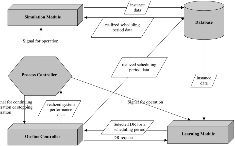
The proposed scheduling system is an intelligent scheduling mechanism that employs machine learning capabilities from AI as well as the process control chart concept from quality control. The goal of the system is to select the best DR among Candidate Dispatching Rules (CDRs) for a particular scheduling period. The general structure is shown in Figure 3.1.
In the proposed system, there are five main subroutines, called modules. They operate in harmony to achieve the goal of selecting the best performing dispatching rule for each scheduling period. The operations of these five modules are as follows. The database provides necessary data for both the learning module and the simulation module. It holds the instance data for the learning algorithm to generate the learning tree. The realized scheduling period data is also stored in the database for assessment of DRs via simulation. Simulation module is used to measure the performances of the candidate dispatching rules. The simulation module is invoked by the process
controller module whenever necessary. Simulation module’s outputs (instance data)
are sent to the database. These results are then used by the learning module to generate the learning tree. Whenever a scheduling decision is to be made according to the current scheduling strategy (e.g., hybrid approach), the learning tree selects a new dispatching rule and this decision is implemented by on-line controller module (i.e., it employs the selected DR in actual manufacturing conditions). It also supplies the realized scheduling period data to the database and monitors the real system for new rule selection symptoms. The process controller module monitors the performance of the learning tree. It takes its inputs (realized average tardiness) from the on-line controller module and monitors the performance of the learning tree. When the performance of the current learning tree is found to be insufficient, it requests from
Signal for operation
Signal for continuing Signal for operation
operation or stopping operation
DR request
Figure 3.1: Proposed System – General Structure Simulation Module Database instance data instance data realized scheduling period data realized system performance data Learning Module On-line Controller Selected DR for a scheduling period Process Controller realized scheduling period data
the simulation module to provide new training data (instance data) for the learning module and then sends a signal to the learning module to update the current learning tree with this new data set. As a result, new dispatching rules are selected from this updated learning tree and the process continues in this manner.
3.3. Scheduling Strategy
The scheduling strategy employed in this research is composed of two critical decisions: how-to-schedule and when-to-schedule. They are explained below:
3.3.1. How-to-schedule
How-to-schedule decision determines the way in which the schedules are revised or updated. As discussed in Sabuncuoglu and Goren (2003), there are mainly three issues: scheduling scheme, amount of data used, and type of the response. The scheduling scheme can be off-line, on-line, or a combination of the two (i.e., hybrid).
Off-line scheduling refers to scheduling all of available jobs for the entire scheduling
period before the execution of the schedule. On the other, hand on-line scheduling is to take scheduling decisions one at a time during the execution of the schedule (e.g. scheduling via priority dispatching rules). Between these two extremes, hybrid or quasi-online scheduling lies. In quasi-online scheduling, a subset of the jobs is scheduled off-line and the rest of the schedule is developed as time goes on. The second issue is related to the amount of data used during the schedule generation process. This can be full or partial, where all the forecasted data is used in the former case whereas only a proportion of the available data is used in the partial case. The third issue is the type of the response. This is related to the question of “what should be done if the current schedule begins to perform worse”. One possibility can be rescheduling, where a new schedule obtained from scratch. Another alternative can be
to take no corrective action (i.e., letting the system recover itself from the negative effects of disruptions). In addition, match-up scheduling or right/left shifting the remaining jobs can also be used for a type of response.
Our implementation is based on the on-line scheduling scheme. Specifically, DRs are selected by the learning tree and the scheduling decisions are made one at a time using these selected rules (see Table 3.1). In terms of the amount of data, we apply the “full” scheme, since all available information about the real manufacturing system is utilized to select a DR for a scheduling period. As the type of the response, we use “reschedule” option, as a new DR is selected at any time when the existing DR is found to be poor.
Table 3.1: Parameters of how-to-schedule
Scheduling Scheme On-line
Amount of Data Full
Type of Response Reschedule
3.3.2. When-to-schedule
“When-to-schedule” determines the responsiveness of the system to various kinds of disruptions. As discussed in Sabuncuoglu and Goren (2003), there are different alternatives to decide on the timing of scheduling decisions. The first way is to schedule the system periodically, which is called as periodic scheduling. In periodic scheduling, the time intervals can be constant or variable. In the former case, schedule revisions are made at the beginning of fixed time intervals. In the latter case, revisions are made after a certain amount of schedule is realized. Another alternative, which is called continuous scheduling, updates the schedule after a number of random
events occur such as machine breakdowns, or a new job arrival, etc. In adaptive
scheduling, a scheduling decision is made after a predetermined amount of deviation
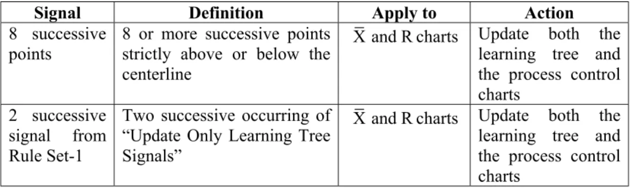
from the original schedule is observed. For example, a scheduling decision is triggered when the difference in average tardiness between the initial and the realized schedules exceeds a threshold value, say 10 minutes. There are also hybrid approaches, which are combinations of the above strategies, and in this research such a hybrid approach is employed for “when-to-schedule” decisions. In our hybrid approach, two different triggering events, called as New Rule Selection Symptoms, are defined for the time of selecting a new DR. These new rule selection symptoms and their definitions are given in Table 3.2.
Table 3.2: New Rule Selection Symptoms
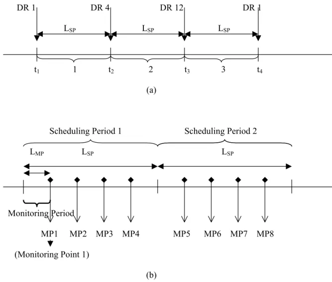
The length of a scheduling period (LSP) is a decision variable and a new DR is
selected at the beginning of each period to carry out the dispatching process until the end of that scheduling period. As seen in Figure 3.2-a, the beginning of each scheduling period is a triggering event for selecting a new DR. However, a selected DR is not always used until the end of a scheduling period because of the existence other symptoms, MP, that may occur in the scheduling process. In such cases, a new DR is selected before the end of a scheduling period.
Abbreviation Name Description
BSP Beginning of each Scheduling Period
Triggers the selection of a new DR at the beginning of each new scheduling period.
MP Monitoring Points Triggers the selection of a new DR at the monitoring points whenever necessary.
DR 1 DR 4 DR 12 DR 1 LSP LSP LSP
t1 1 t2 2 t3 3 t4
(a)
Scheduling Period 1 Scheduling Period 2 LMP LSP LSP
Monitoring Period
MP1 MP2 MP3 MP4 MP5 MP6 MP7 MP8 (Monitoring Point 1)
(b)
Figure 3.2: Representation of Rule Selection Symptoms. (a) New Rule Selection Symptom (BSP). (b) Monitoring Period and Monitoring Point
As seen in Figure 3.2-a, the performance of the current DR is monitored regularly at monitoring points and if it is found to be poor (i.e., the performance is worse than a certain percentage of the desired level), a new DR is requested from the learning tree. The length of a monitoring period (LMP) is usually a decision variable
(or policy variable) and a complete scheduling period contains a fixed number of monitoring points. LMP=LSP/(k+1), where k is the number of monitoring points in a
DR5 DR7 DR3
Scheduling Period 1 Scheduling Period 2 Scheduling Period 3 LMP LSP < LSP t1 t2 t3 t4 t5 t6 t7 Monitoring Period MP1 MP2 MP3 MP4 MP5 MP6 MP7 MP8 … f(MP1) < χ f(MP5) < χ (b) f(MP2) < χ f(MP6) > χ f(MP3) < χ f(MP4) < χ (a)
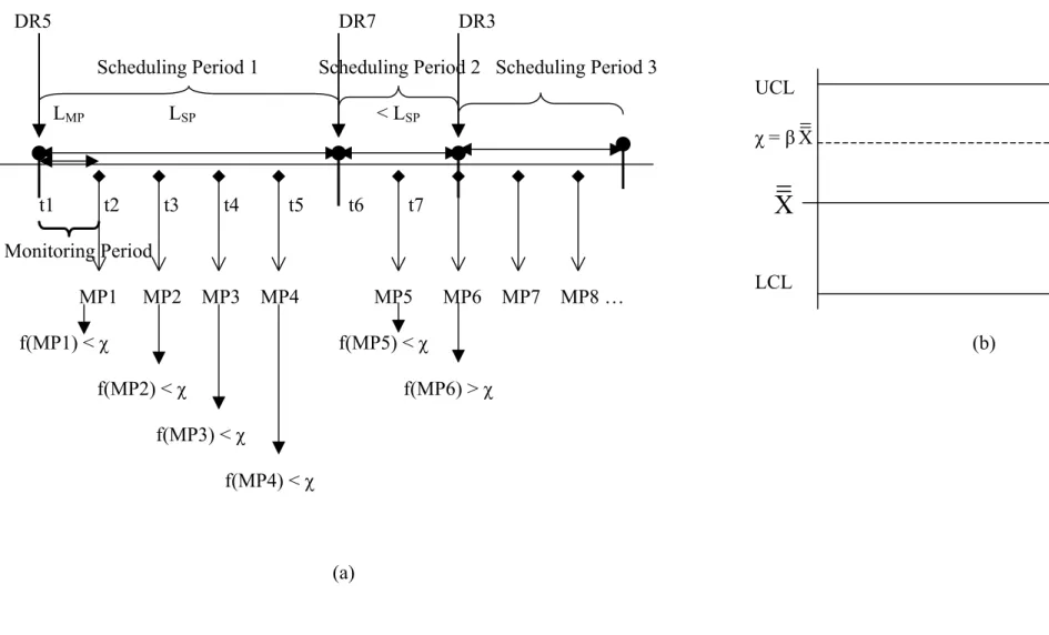
Figure 3.3: Rule Selection Symptoms. (a) New Rule Selection Symptom (MP). (b) Representation of χ in control. χ = βΧ
UCL
LCL
Χ
As an example, consider the case in Figure 3.3, which displays the MP symptom and the actions to be taken. At every monitoring point in a scheduling interval, the current value of the performance measure is compared with a threshold value. If it is worse than the threshold, a new DR is requested from the learning tree. Otherwise, the system continues with the current DR. In Figure 3.3, in none of the monitoring points of the scheduling period 1 there is a need for a change and hence DR5 is used throughout the scheduling period 1 (i.e., type complete). At the beginning of scheduling period 2 (at t6), DR7 is selected as a new rule by the learning tree. At the monitoring point 6, its performance f(MP6) is found to be worse than the threshold value χ, and a new DR is requested from the learning tree. Based on the learning tree recommendation, DR3 is assigned as the new DR for the scheduling period 3. Note that the scheduling period 2 is now of type incomplete, since its length is less than LSP.
The function f(*) gives simply the average tardiness value of the completed jobs from the beginning of the current scheduling period. For example, f(MP2) is the average tardiness of all the jobs completed between the times t3 and t1, and f(MP5) is the average tardiness of all the jobs completed between the times t7 and t6 (see Figure 3.3). As seen in Figure 3.3-b, the threshold value χ is a multiple of the expected average tardiness (χ = βΧ , where the parameter β is 0<β and Χ is the long-run expected average tardiness).
3.4. Data Structures
There are different data types used in the proposed scheduling system. These are explained below.
3.4.1. Performance Data (Realized System Performance)
Performance Data is the data type that represents the performance of a DR in a
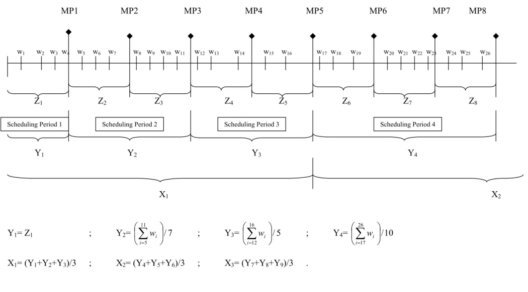
specific scheduling period in terms of tardiness, average tardiness and the average of average tardiness. These data are used for different purposes but in the following formats. We define three different formats for performance data as: monitoring period
performance (Z), scheduling period performance (Y), and aggregated performance
(X). In Figure 3.4, each of these data structures are displayed in detail. Each wi value
is an individual tardiness value of a completed job. Monitoring period performance (Z values) is the average tardiness of all the completed jobs between the last monitoring point and the current monitoring point. For example, Z1=(w1 + w2 + w3 + w4) / 4 for
MP1, and Z2= (w5 + w6 + w7) / 3 for MP2. In other words, the Zi values are the
average tardiness realized in a monitoring period. Scheduling period performance (Y values) is the average tardiness of all the completed jobs in a scheduling period. For example, Y1= Z1, and Y4= 10/ 26 17
∑
= i iw . Note that scheduling period 1 is of type
incomplete and contains only one monitoring period whereas scheduling period 4 is of type complete and consists of three monitoring periods (in this illustrative example a complete scheduling period is assumed to contain three monitoring periods). In other words, the Yi values are the average tardiness realized in a scheduling period.
Aggregated performances, Xi values, are samples of Yi values. In Figure 3.4, each Xi
value is defined as the average of three Yi values (the number of Yi values to be
grouped is a parameter) and therefore X1= (Y1+Y2+Y3)/3, X2=(Y4+Y5+Y6)/3, X3=
(Y7+Y8+Y9)/3. In other words, aggregated performance is the average tardiness
MP1 MP2 MP3 MP4 MP5 MP6 MP7 MP8 w1 w2 w3 w4 w5 w6 w7 w8 w9 w10 w11 w12 w13 w14 w15 w16 w17 w18 w19 w20 w21 w22 w23 w24 w25 w26 Z1 Z2 Z3 Z4 Z5 Z6 Z7 Z8 Y1 Y2 Y3 Y4 X1 X2 Y1= Z1 ; Y2= 711 / 5
∑
= i i w ; Y3= 516 / 12 ∑
= i i w ; Y4= 1026 / 17 ∑
= i i wX1= (Y1+Y2+Y3)/3 ; X2= (Y4+Y5+Y6)/3 ; X3= (Y7+Y8+Y9)/3 .
Figure 3.4: Types of Performance Data
Among these data structures, the Zi values are used for monitoring the
performance of the current DR at monitoring points. Yi values are used as the
performance value of the DR that is used in a specific scheduling period. It is also a part of the realized scheduling period data, which is used by the simulation module. Finally, the Xi values are used for the performance evaluation of the existing learning
tree and these are the data that are plotted on the Χ chart. Yi values are aggregated to
form Xi values because of the normality assumption requirement of the control chart.
Aggregating four to six data is sufficient for meeting this requirement.
3.4.2. Instance Data
Figure 3.5 shows the representation of instance data. Each row in this figure corresponds to an individual data, which has a number of attributes, the class value that indicates the best DR that works under these specific attribute-value combinations and the performance value (scheduling period performance) of that DR.
Figure 3.5: Instance Data Representation
These data are created from the outputs of the simulation module and are used for two important reasons in the system. First, it is used in the construction of the learning tree, where these data are supplied to the learning algorithm to make inferences about the characteristics of the manufacturing system based on the pre-specified set of attributes. Second, it is used to construct the process control charts. The column that stores the performance values is supplied to the process controller module whenever the process control charts are to be updated. In the second usage of
Attribute-1 Attribute-2 … Attribute-n Performance Value Class Value A-1 Value A-2 Value … A-n Value f(DR3) DR3 A-1 Value A-2 Value … A-n Value f(DR5) DR5 A-1 Value A-2 Value … A-n Value f(DR7) DR7
… … … …
the instance data, only the performance value column is used. This column contains the best performance values found by the simulation module under different DRs based on the specified attribute values. These data points are represented as *
i
X
indicating the best performances (average tardiness) found for specific system conditions. Since, we monitor the performance of the learning tree relative to the best performance; we employ *
i
X values when constructing the process control charts (for
detailed information about f(DRj) see section 3.5.2. Simulation Module).
3.4.3. Realized Scheduling Period Data
In Figure 3.6, the realized scheduling period data structure is depicted. At the end of any scheduling period, the on-line controller module sends all the relevant realized manufacturing system data to the database. These data points include the values of the system attributes at the beginning of the scheduling period (scheduling period k in our case), the realized random events during that period as well as the average tardiness value obtained under the current DR in use in that scheduling period. In the current implementation, since we model actual manufacturing conditions in a simulation model, we store the seed values of the random number generations for each stochastic variable in this column. Thus, the entire history is easily generated using these seeds when necessary. Hence, these data points are the result of the tracking of the system by the on-line controller. The importance of this data type comes from the following fact: when a DR is selected by the learning tree and used in a scheduling period, we do not know whether it is actually the best DR for that scheduling period. The only way to know it is to simulate the other DRs in the CDR set under exactly the same system conditions. These data points provide an important feedback for the system to
improve the quality of the learning tree whenever necessary (these issues will be discussed later in the text).
Scheduling Period Attribute-1 Attribute-2 … Attribute-n Realized Scheduling Period Data 1 A-1 Value A-2 Value … A-n Value Realized Scheduling
Period-1 Data 2 A-1 Value A-2 Value … A-n Value Realized Scheduling
Period-2 Data
… … … …
k A-1 Value A-2 Value … A-n Value Realized Scheduling Period-k Data
Figure 3.6: Realized Scheduling Period Data
3.5. Proposed System – A Detailed Explanation
General structure of the proposed system has been introduced in Section 3.2. We now explain each module in detail.
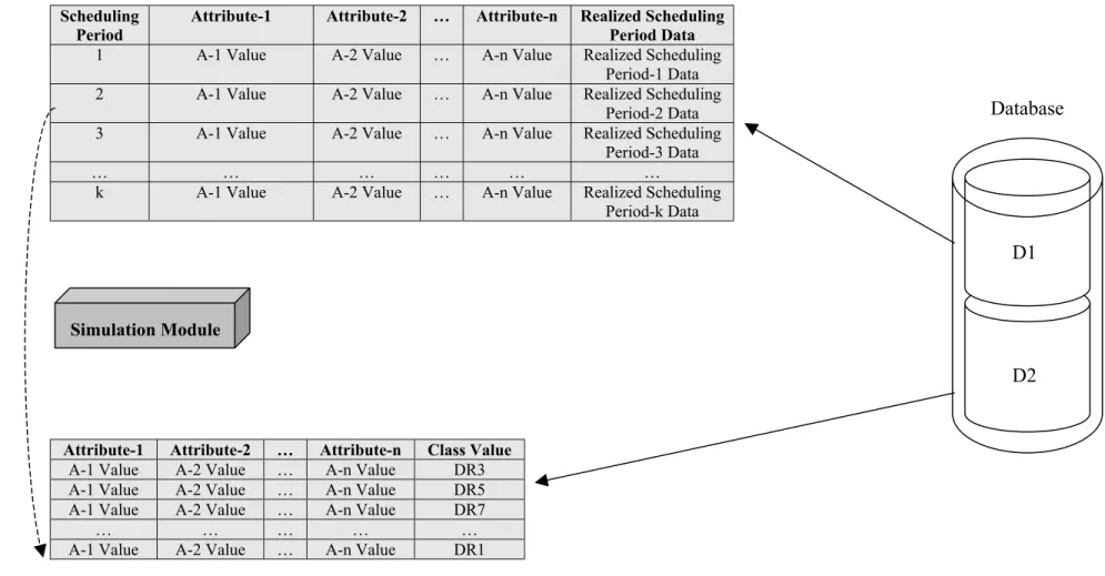
3.5.1. Database
The database of the proposed system is composed of two layers, called as D1 and D2 (Figure 3.7). D1 stores the “realized scheduling period data” discussed in Section 3.4.3. These data are supplied from the on-line controller to the simulation module. D2 stores the instance data discussed in Section 3.4.2. These data are supplied from the simulation module, and are used by the learning module to generate the learning tree.
As stated earlier, D1 stores the input data for the simulation module and D2 stores the output data of the simulation module. Hence, whenever a row of data from D1 is used in the simulation module, it is deleted from D1 and an associated row of the output data is added to D2. For example, in Figure 3.7, row 2 of the table in D1 is deleted from the table when it is used by the simulation module and the last row in the table of D2 is created (as indicated by dashed lines).
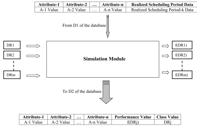
3.5.2. Simulation Module
The simulation module is activated upon the request by the process controller module to measure the performance of all DRs for the past scheduling periods (using the realized scheduling period data) and to generate new training sets for the learning module. In this way, the quality of the DRs used for the past periods is also assessed.
In Figure 3.8, scheduling period-k (one of the past scheduling periods) is simulated for all m DRs. Previous historical data stored in the D1 are used to generate input to simulation experiments. All m DRs are simulated one by one and their corresponding average tardiness values (f(DRj)) are measured. Then, the DR that results in the minimum average tardiness value (DRj = DR[argmin{f(Dri), i = 1,2,3,…,m}]) is identified as the best DR for scheduling period-k. Note that this rule may not be the same rule used previously for period-k. Running the simulation module for past periods and collecting the performance data help us to create training sets for the learning module. Hence, the best rule identified in the simulation experiments and the corresponding manufacturing conditions are stored in D2 of the database in the form of instance data (see Figure 3.8).
3.5.3. Learning Module
The learning module is mainly composed of two parts: “learning module-1” and “learning module-2”. Their functionalities are given below:
Learning Module-1: This module contains the learning tree that is
constructed by the learning algorithm in learning module-2. Its responsibility is to select a new DR from the existing learning tree based on the current values of the system state attributes. The on-line controller module provides the current values of these attributes to learning module-1 and requests a new DR. In response, module-1 recommends the best DR to the on-line controller (Figure 3.9).
Database
Figure 3.7: Database of the Proposed System Scheduling
Period Attribute-1 Attribute-2 … Attribute-n Realized Scheduling Period Data
1 A-1 Value A-2 Value … A-n Value Realized Scheduling
Period-1 Data
2 A-1 Value A-2 Value … A-n Value Realized Scheduling
Period-2 Data
3 A-1 Value A-2 Value … A-n Value Realized Scheduling
Period-3 Data
… … … …
k A-1 Value A-2 Value … A-n Value Realized Scheduling
Period-k Data
Attribute-1 Attribute-2 … Attribute-n Class Value
A-1 Value A-2 Value … A-n Value DR3
A-1 Value A-2 Value … A-n Value DR5
A-1 Value A-2 Value … A-n Value DR7
… … … … …
A-1 Value A-2 Value … A-n Value DR1
D2 D1
Attribute-1 Attribute-2 … Attribute-n Realized Scheduling Period Data A-1 Value A-2 Value … A-n Value Realized Scheduling Period-k Data
Figure 3.8: Simulation Module
Attribute-1 Attribute-2 … Attribute-n Performance Value Class Value
A-1 Value A-2 Value … A-n Value f(DRj) DRj
DR1 DR2 DRm f(DR1) f(DR2) f(DRm)
From D1 of the database
To D2 of the database
DRj
Figure 3.9: Learning Module
Attribute-1 Attribute-2 … Attribute-n Class Value
A-1 Value A-2 Value … A-n Value DR3
A-1 Value A-2 Value … A-n Value DR5
A-1 Value A-2 Value … A-n Value DR7
… … … … …
A-1 Value A-2 Value … A-n Value DR1
Attribute-1 Attribute-2 … Attribute-n
A-1 Value A-2 Value … A-n Value
CURRENT Learning Tree
C4.5 Learning
Algorithm
D2 Database D1 DatabaseLearning
Module-1
Learning
Module-2
On-line Controller New TreeLearning Module-2: This module contains the learning algorithm that is used
to generate the learning tree in learning module-1. As seen in Figure 3.9, the algorithm is invoked by the process controller module and the necessary data (instance data) is retrieved from the D2 database. C4.5 algorithms (Quinlan, 1993) are used to create the learning tree (see Figure 3.9).
3.5.4. On-line Controller
As discussed in Section 3.2, there are mainly two responsibilities of the on-line controller. These are as follows:
i) Handling the realization of a scheduling decision
Realization of a scheduling period is accomplished by the implementation of a scheduling decision (i.e., implementation of a dispatching rule) in either a real manufacturing system or a simulated environment. In this study, we use the second approach and run the internal simulation engine (see Figure 3.10). To get a realization of a scheduling period, on-line controller requests a DR from the learning module and implements it. The results of implementation in the form of realized scheduling period data is sent to D1 of the database.
ii) Monitoring the real system for new rule selection symptoms
Detecting new rule selection symptoms (see Table 3.2 on page 20) and taking the appropriate actions in response to the existence of these symptoms is another functionality of the on-line controller module. As discussed in Section 3.3.2 (Figures 3.2 and 3.3 in particular), there are two new rule selection symptoms (BSP and MP). Whenever the on-line controller module detects any one of these two symptoms during the realization of a scheduling period, it pauses the execution process and requests a new DR from the learning module. Upon the new DR supplied by the
learning module-1, on-line controller resumes the execution process with this new DR (see Figure 3.10).
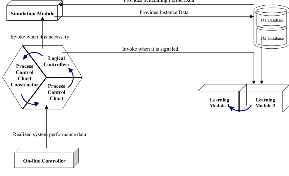
3.5.5. Process Controller
Process controller coordinates the operations of the other modules. It takes its necessary inputs from the on-line controller and activates the other three modules appropriately. It has three sub-modules: process control chart constructor, process control chart, and logical controllers (see Figure 3.11). These are explained in detail as follows:
i) Process Control Chart Constructor
The purpose of this sub-module is to update the process control charts ( and RΧ charts), which are responsible from the control of the learning tree. The construction of the process control charts requires data ( *
i
X ) from D2 (the
construction methods of these two charts are given in Appendix A).
The Χ chart is used to detect the shifts in the mean performance of the decisions (selected DRs) given by the learning tree. Averages of the average tardiness values are plotted in this chart. R chart is used to detect the shifts in the variance of the performance of the decisions of the learning tree (see DeVor et al., 1992). In other words, standard deviations of the average tardiness values of the realized scheduling periods are plotted in this chart.
ii) Process Control Chart Sub-module
This module contains the process control charts, which are created by the process control chart constructor module (Figure 3.11). The purpose of this module is to handle the monitoring operation of the learning tree by using these two charts ( and RΧ charts).
On-line Controller
Simulator
Learning Module D2 Database D1 Database Realized Scheduling Period Data Logical Subroutines DROne of the distinguishing features of the proposed scheduling system from the previous studies (Suwa et. al., 2003 and Shaw et. al., 1992) is the mechanism that continuously updates the learning tree. This continuous update is important since the manufacturing system often undergoes various types of changes in time. In this context, the process control charts act as a regulator of the learning tree. Moreover, the process control charts may also need to be updated due to changes in manufacturing conditions. Hence, as the proposed system evolves over time, two important decisions need to be made:
Decision-1: Is it necessary to update the existing learning tree at current time t? Decision-2: Is it necessary to update the existing process control charts at current time t?
These two questions are to be answered every time when a new data point is plotted in the process control charts ( and RΧ charts) and the decisions are made by the rules defined in the logical controllers of the process controller module. These rules are defined in the next section. In this section, however, we focus only on the data plotted on the process control charts. Recall that the data plotted on the
and R
Χ charts are obtained from the on-line controller (the Χ data) but the data i used to update the charts are supplied from the D2 database.
In Figure 3.12, we illustrate the data points plotted on the Χ chart. The horizontal axis represents the time and the vertical axis is the average tardiness (i.e., performance measure). When the system continues, the Yi values (average tardiness
per scheduling period) are collected by the on-line controller at the end of each scheduling period. These observations are then grouped in size 5 to create X ’s i
Provides Scheduling Period Data
Provides Instance Data
Invoke when it is necessary
Invoke when it is signaled
Realized system performance data
Figure 3.11: Process Controller Module and Its Relationships with Other Modules Process Control Chart Constructor Process Control Chart Logical Controllers Simulation Module D2 Database D1 Database Learning Module-1 Learning Module-2 On-line Controller
Y1 Y2 Y3 Y4 Y5 Y6Y7Y8 Y9Y10Y11Y12Y13Y14Y15Y16Y17Y18Y19Y20Y21Y22……… Y66 Sample mean X1 X2 X3 X4 X5 X6 X7 X8 X9 X10 X11 X12 X13 X14 X15 X16 X17 X18 X19 X20 + + + + + A + + + + 3σ B + + + + C + + + + Χ + C + + + 3σ B A +
Change the learning tree Change the learning tree Change the learning tree Change the process control chart