Modeling the economic effects of banking sector regulation and supervision

(1)

MODELING THE ECONOMIC EFFECTS OF BANKING SECTOR REGULATION AND SUPERVISION

A Master’s Thesis by GONCA ŞENEL Department of Economics Bilkent University Ankara August 2007

(2)

(3)

The Institute of Economics and Social Sciences of

Bilkent University

by

GONCA ŞENEL

In Partial Fulfillment of the Requirements for the Degree of MASTER OF ECONOMICS

in

THE DEPARTMENT OF ECONOMICS BILKENT UNIVERSITY

ANKARA

(4)

I certify that I have read this thesis and have found that it is fully adequate, in scope and in quality, as a thesis for the degree of Master of Arts in Economics

--- Assoc. Prof. Bilin Neyaptı Supervisor

---

Assoc. Prof. Zeynep Önder Examining Committee Member

---

Assist. Prof. H. Çağrı Sağlam Examining Committee Member

Approval of the Institute of Economics and Social Sciences

--- Prof. Erdal Erel Director

(5)

ABSTRACT

Şenel, Gonca Master of Economics

Supervisor: Assoc. Prof. Bilin Neyaptı

August 2007

In this thesis, the effect of bank regulation and supervision on economic growth is analyzed theoretically. By means of OLG model framework, optimization problems of three types of agents have been constructed: consumer’s utility maximization problem, producer’s and bank’s profit maximization problems. Two types of settings have been evaluated separately in order to figure out the monitoring decisions of the bank: homogenous producers and non-homogenous producers. Regulation and supervision level of the banking sector is represented by an index, which is denoted by α in the model and it affects the optimization behavior of each agent: it increases the amount of deposits transferred to banks by consumers; it enhances the amount of credit that is converted into capital, and it affects behaviors of the bank in terms of monitoring producers. Calibration analysis is performed and it is found that no monitoring is more preferable for the bank as compared to monitoring and variable cost monitoring is more preferable than fixed cost monitoring. In addition, comparative static analysis yield that

(6)

higher bank regulation and supervision improves per capita output, wages and credit and reduces interest rates and producers with higher credit conversion capabilities have higher per capita output; they pay higher wages; they demand more credit and pay less interest rate.

(7)

ÖZET

BANKACILIK SEKTÖRÜ DENETLEME VE GÖZETİMİNİN EKONOMİK ETKİLERİNİN MODELLENMESİ

Şenel, Gonca

Yüksek Lisans, İktisat Bölümü Tez Danışmanı: Doç. Dr. Bilin Neyaptı

Ağustos 2007

Bu tezde, banka denetleme ve gözetiminin ekonomik gelişmeye olan etkisi teorik olarak incelenmiştir. Çakışan Nesiller modeli çerçevesinde üç çeşit bireyin eniyileme problemleri kurulmuştur: tüketicinin yarar eniyileme problemi, üreticinin ve bankanın kar eniyileme problemi. Bankanın denetleme kararlarını çözebilmek amacıyla iki durum birbirinden ayrı olarak değerlendirilmiştir: türdeş üreticiler ve türdeş olmayan üreticiler. Modelde α ile ifade edilen bankacılık sektörü denetleme ve düzenleme derecesi bir endeksle gösterilmektedir ve her bireyin eniyileme davranışlarını etkilemektedir: tüketicilerin bankalara yatırdıkları tüketicilerin mevduat miktarını arttırır, sermayeye dönüşen kredi miktarını yükseltir ve bankanın üreticileri denetleme davranışlarını etkiler. Kalibrasyon analizleri yapılmış ve bankalar için üreticileri denetlememek denetlemeye nazaran ; değişken maliyetli denetleme de sabit maliyetli denetlemeye nazaran daha tercih edilir bulunmuştur. Bununla birlikte, karşılaştırmalı statik analizleri yapılmış ve bu analizler daha yüksek seviyede bankacılık denetleme ve düzenlemesinin

(8)

daha yüksek kişi başına gelir, ücret ve kredi sağladığını; faiz miktarlarını düşürdüğünü; aynı zamanda daha yüksek kredi dönüştürme becerisine sahip olan üreticilerin daha yüksek ücret ödediğini, daha fazla kredi talep ettiğini ve daha düşük faiz ödediğini ortaya koymuştur.

(9)

ACKNOWLEDGEMENTS

I would like to thank to Prof. Bilin Neyaptı for her continuous supervision and invaluable guidance. I am truly grateful to her for her patience, support and enthusiasm that motivated me at each phase of this thesis

I would like to thank to Prof. Zeynep Önder for helping and encouraging me continuously from the beginning of my academic life in Bilkent

I am indebted to Prof. H.Çağrı Sağlam for always being ready to help and for his insightful comments and guidance.

I owe special thanks to my father, Cemali Şenel, for always being ready to listen; my mother Mualla Şenel for supporting me throughout my whole life, and my brother Şinasi Şenel, for helping me see the glass half full.

I would like to thank to Nida Çakır for her invaluable comments and continuous help, but especially for her friendship.

Finally, I would like to thank to my friend Musab Kurnaz for his patience, sensibility and benevolence.

(10)

LIST OF TABLES

Table 1: Timing of Events ... 23 Table 2: Simulation of the profit functions under fixed cost and variable cost monitoring and no-monitoring for 0 ≤ ≤ 1α and β <0.5 ... 51

(13)

LIST OF FIGURES

Figure 1: FM-NM for β =0.45... 52 Figure 2:VM-NM for β =0.45 ... 52 Figure 3: FM-VM for β =0.45... 53 Figure 4: FM-NM for β =0.4... 53 Figure 5: VM-NM for β =0.4... 54 Figure 6: FM-VM for β =0.4... 54 Figure 7: FM-NM for β =0.35... 55 Figure 8:VM-NM for β =0.35 ... 55 Figure 9: FM-VM for β =0.35... 56 Figure 10: FM-NM for β =0.3... 56 Figure 11:VM-NM for β =0.3 ... 57 Figure 12: FM-VM for β =0.3... 57 Figure 13: FM-NM for β =0.25... 58 Figure 14:VM-NM for β =0.25 ... 58 Figure 15: FM-VM for β =0.25... 59

(14)

LIST OF SYMBOLS

α : bank regulation and supervision level

t

S−1: total amount of savings

t-w1: wage rate

t 1

s₋ : amount of savings of each consumer s_t-₁+c_t-₁≤w_t-₁+ −(1 α)cr_t-₁

t-1

c : consumption of each consumer

t -1

d : amount of deposits collected from each consumer ( d_t-1=αs_t-1)

(1+r_dt): interest rate paid to the consumers by the bank

t

Y: real output

t

K : capital used in production Yt AK Lt t

β 1−β

= t

L : labor used in production

i

p: individual moral hazard rates (distributed uniformly between 0 and 1, 1 indicating

no moral hazard)

t

CR : amount of credit extended to producers by the bank (in case of homogenous

(15)

(1+ : interest rate paid to banks by producers in case of homogenous producersrt) (1+r_it): interest rate paid to banks by producers in case of non homogenous producers

cr: per capita credit extended to producers by the bank (cr:CR

L )

( )

ψ α : fixed monitoring cost ( )

(16)

CHAPTER I

INTRODUCTION

Importance of financial intermediaries on economic activities has long been known by economists. Beginning with Schumpeter (1912), it has been realized that financial intermediaries foster economic growth by facilitating investment. When there are costs involved in economic transactions between individuals, financial intermediaries handle these costs better than individuals since they can pool risk and control borrowers by monitoring. They benefit from economies of scale so that they are able to allocate the resources efficiently.

Considering the relationship between financial development and economic growth, there is a vast amount of work showing the importance of financial intermediaries on economic growth, and most of them show strongly that financial sector development is an important aspect on promoting growth. Greenwood and Jovanovic (1990) and Benchivenga and Smith (1991) show the existence of this

(17)

relationship theoretically by using endogenous growth models. Besides the theoretical work, many studies (for example, King and Levine (1993), and Levine (1997)) empirically show that there is robust and significant relationship between financial system development and economic growth.

In addition to the analysis of the financial sector development and growth relationship, economists also focus on the effect of the banking sector on the economy specifically. These studies reveal that by allocating resources to the most “appropriate candidates” by managing risk and monitoring borrowers, banks increase the efficient use of resources leading to economic growth. On this aspect, Townsend (1979) and Stiglitz and Weiss (1981) construct the theoretical background of banking theory.

Considering banks’ decision process we can say that banks are among the most influential agents in the economy who verify “appropriateness” of candidates that help transform savings into investment. Therefore, well functioning of banks is very important for economic growth, and regulation and supervision (RS) of banks is an important concern for banks to sustain their performance by controlling investment decisions in terms of risk and effectiveness.

This is the first study that examines RS and growth relationship theoretically and it is motivated mainly by Neyaptı and Dinçer (ND, 2005), who measure countries’ regulation and supervision (RS) based on the letter of banking laws. From these measurements, ND construct country-specific RS indices that they use to test the relationship between RS and growth. The test results show that there is a positive and

(18)

robust relationship between RS level and economic growth in transition economies. Barth et al. (2004) also measure RS, using a different methodology and based on questionnaires, finding positive association between RS and bank stability and performance.

In our study, we aim to investigate the existence of this relationship using a model-based approach. We use the 2-period OLG model setting with three types of agents: consumers, producers and banks, where banks are the only source of the credit. The economy has a predetermined RS level ( )α that is in the same spirit as the country-specific RS index of ND1. The model is set such that the α level affects all types of the agents from different aspects: it increases the portion of savings that are put in to the banks as deposits, it increases the portion of the credit that is converted into capital, and it affects (positively) the decision of the bank to monitor borrowers. We also consider two different settings, where producers are homogenous and non-homogenous in terms of their credit conversion capabilities so that we are able to examine the effect of individual moral hazard rates and RS on the economy.

The findings of our study indicate that RS positively affects the economy; it increases the production, per capita capital and wages at the same time. In addition, we also investigate the effect of RS on bank decision process and find that different RS levels change the tendency of banks to monitor the agents.

1_{RS in ND is formed based on the “intensity” of various aspects of legal provisions, including capital}

requirements, lending, ownership structure, directors and managers, reporting/recording requirements, corrective action, supervision and deposit insurance.

(19)

The organization of the remainder study is as follows: In Chapter 2, we examine the literature on the relationship between financial sector development and economic growth; in Chapter 3, we propose a model to analyze the effect of RS on the economy; in Chapter 4, we interpret our results emerging from the model solution; and Chapter 5 concludes and outlines the extensions that will be undertaken.

(20)

CHAPTER II

LITERATURE REVIEW

In Arrow-Debreu world, information is symmetric and frictionless in terms of information flow and markets are complete. In this setting, there is no need for financial intermediation since the agents can obtain information and do the transactions by themselves without incurring any cost (Levine, 1997 and Santos, 2001). However, in the actual world, these activities carry costs that the individuals cannot bear alone. This situation leads to the formation of financial intermediaries in order to carry out the transactions.

The main goal of a financial intermediary is to reallocate the resources of economic units with surplus (savers) to economic units with funding needs (borrowers) (see Allen and Santomero, 2001). According to Levine (1997), the functions of financial intermediaries are allocating the resources, mobilizing savings, managing risk and ensuring corporate control by monitoring. Similarly, in Bhattacharya and Thakor (1993)

(21)

the roles of financial intermediaries are summarized as: reducing the costs of transactions, benefiting from economies of scale by increase in size, increasing the quality and level of investment, giving signals about the quality of the borrower. From these definitions it can be realized that financial intermediaries play an important role in overcoming the information and transaction costs. Accordingly, it can be claimed that these institutions affect the system and lead to economic growth by improving resource allocation decisions and investment quality. On this matter, the finance-growth literature offers three different views (see Levine, 2003 and 1997).

According to the first view, in the essays of Meier and Seers (1984), authors do not even mention the financial system as one of the explanatory variables leading to economical growth since they think that it is not worth to do so (see Levine 2003). In addition to this, Lucas (1988) also claims that role of the financial sector on growth is overemphasized.

The second view, pioneered by Robinson (1952), claims that finance follows growth rather than the reverse relation. She claims that development in economy creates a need for the development in financial sector that in return leads to economic growth.

The third perception has roots at the beginning of the 20th_{century; Schumpeter} (1911) emphasizes the importance of development of financial system on economic growth (see Levine, 1997). Schumpeter claims that financial system fosters economic growth by promoting technological innovation. Financial intermediaries are able to identify and fund successful innovative products and processes that in return lead to

(22)

growth in the economy. They are better suited for these functions than individuals due to economies of scale that lowers transaction and information costs.

Early theoretical research on finance and growth relation can be listed as Patrick (1966), Cameron (1967), Goldsmith (1969), McKinnon (1973), and Shaw (1973). With the emergence of endogenous growth literature, which is pioneered by Romer (1986 and 1990), Lucas (1988) and Rebelo (1991), these models started to be extensively used in explaining the relationship between financial development and economic growth in general equilibrium models. Greenwood and Jovanovic (1990) present the first theoretical work that attempts to explain the finance-growth relationship by using the endogenous growth theory. In their work, they aim to explain two important issues related with growth, finance and income distributions. Firstly, they find support for Kuznets’s (1955) hypothesis on growth and income distribution. In this theory, difference in income levels widens as the economy experiences a fast-growth and then this difference vanishes as the economy becomes stable. Secondly, they theoretically show these stages and differences. By means of endogenous growth theory, they also claim that there is an interrelation between finance and growth rather than a one direction causal relationship. They show that economic growth helps agents use costly financial structures, what we can call as financial development, and, as a response, financial development fosters growth. As a further study, Townsend and Ueda (2005) take this model as base and explore economies in transition with further calibration.

Benchivenga and Smith (1991) show financial structure-growth relationship in a different setting, again using endogenous growth models. Different from Greenwood

(23)

and Jovanovic (1990), they use overlapping generations’ model and focus on the effect of competitive financial intermediaries on savings behavior. Upon the examination of findings, they report that relationship between financial intermediation and savings behavior is not clear. However, by using this model, they also reach the conclusion that financial intermediation increases economic growth level.

In these two previous models, financial intermediaries achieve economic growth by allocating resources to investments that have high return. Considering characteristics of financial intermediaries we can say that in both of the models, financial intermediation was restricted to banks. Building upon the previous two theoretical models, Greenwood and Smith (1997) develop two models in order to investigate finance-growth relationship. First one is constructed in order to explore the role of a financial intermediary in efficient allocation of funds by ensuring liquidity in the market. This is the improved version of previous Bencivenga-Smith (1991) model. In this version, authors report that “intermediation is necessarily growth enhancing” (p.4). In addition, endogenous formation of equity markets is introduced in the model. In this study, researchers determine the conditions under which both intermediation takes place and equity market is formed. The second model aims at exploring the effect of financial intermediation on specialization. From these two models what they find is that there is a “threshold effect” (similar to Greenwood and Jovanovic, 1990), implying that an economy should be wealthy enough to support financial structure, which then fosters economic growth in turn.

(24)

In another recent study, Khan (2001) is mainly concerned with costs emerging from informational asymmetries. He develops a dynamic equilibrium model in which agents, who have access to external finance, obtain higher returns to investment. This leads other agents to adopt to the current level of technology. Accordingly, he proposes that financial intermediation increases overall net worth of investment.

Studies summarized above are only interested in growth and its interaction with financial intermediation. In addition to these models, Aghion et al. (2005) explore the effects of financial development on cyclical component of investment and accordingly to growth and volatility under the assumption of tight credit constraints. In this study they form a growth model in which firms have two investment options: long-term and short-term investment. With the help of this model, they find that low financial development causes high sensitivity of growth to exogenous shocks and stronger negative effect of volatility on growth.

Considering models aiming at explaining banking theory alone, we observe that Townsend (1979) and Stiglitz and Weiss (1981) are the major papers that construct banking theory by using utility and profit maximization. In their models, asymmetric information plays an important role in resource allocation process (Guzman, 2000). Sharp (1990) considers banking and borrower relationships in a endogenous model. Bernanke et al. (1998) explores the effects of credit frictions on business fluctuations. They examine whether “financial accelerator” increases the effect of the shock in the economy by investment channels and find that there is a positive relationship between financial accelerator and business cycle behaviors.

(25)

The foregoing studies summarize the main models that examine the importance of financial markets with respect to optimal resource allocation and overcoming information costs. As we look at the empirical evidence, we also see that there is strong support for financial intermediaries’ role to amplify growth. As one of the most influential empirical studies King and Levine (1993) explore whether there is a relationship between financial development (defined as four distinct variables) and economic growth (defined as three different variables). They use cross-country analysis and find out that four indicators of financial development ( size of formal financial intermediation sector relative to GDP; importance of banks relative to the central bank; percentage of credit allocated to private firms; and ratio of credit issued to private firms to GDP) are strongly and robustly correlated with the indicators of economic growth (which are per capita GDP growth; rate of physical capital accumulation; and improvements in the efficiency of capital allocation). In addition, they test whether financial development indicators are successful in predicting long run growth. In this study they find that predetermined component of financial development is a good predictor of long-run growth.

King and Levine’s study is successful in explaining the relationship between financial market development and growth, but there is still room for doubt for the direction of causality. Following this study, Jayaratne and Strahan (1996) support the same idea and examine the direction of the causal relationship using a different set of indicators and US data. Using bank branch deregulation as the indicator of financial development, they find evidence that states do not deregulate their financial system

(26)

when they have an expectation of higher growth. This finding indicates that growth does not lead to financial development. In addition, they find that there is significant relationship between financial development and growth. Accordingly, they conclude that financial development promotes economic growth rather than the reverse relation.

The causal relationship between financial development and economic growth is also investigated in Beck et al. (2000). In order to overcome the simultaneity problem, an exogenous determinant of financial development that also has no relationship with economic growth is used as an instrumental variable. Exogenous variable is determined as legal and accounting systems, following LaPorta et al. (1997 and 1998). These variables are shown to be good indicators of financial development and accordingly they are used in growth regression. Result of the regressions shows that there is a robust and significant relationship between growth and exogenous indicators of financial development implying that financial development fosters economic growth.

Beside above studies examining the relationship between financial development and growth has been shown empirically there is also a literature empirically demonstrating the individual importance of bank development on growth. Levine (1998) examines the relationship between legal system, bank development and long run economic growth. In this study, firstly relationship between legal environment and bank development is examined and secondly by using legal environment factor as the exogenous determinant of bank development, relationship between bank development and long run growth has been explored. The legal system information is obtained from LaPorta et al. (1997 and 1998). Levine (1998) finds that legal rights of creditors and

(27)

effectiveness of the enforcement of these rights are among the most important indicators of the bank-development. In addition to this, they find that exogenous component of bank development is positively correlated with long run growth.

In most of the previous studies the effect of banking sector development was used in order to show the finance-growth relationship. Arestis and Demetriades (1997) investigate whether the same relationship holds as financial development is represented by stock market development. In addition to this, they prefer to use time series approach rather than cross-section analysis in order to control for the country-specific effects. In this setting, they find a similar relationship but the results mostly depend on individual countries.

After investigating these studies, which specifically focus on either banking or stock market development, Levine and Zervos (1998) study the effect of banking sector development and stock market development together and test whether their individual relationship with growth is still significant and robust even though they are tested together. In this study, they find out that stock market liquidity and banking development are both positively and robustly correlated with future rates of economic growth. In addition, since banking development and stock market liquidity enter into the same growth regression and they are both significant, it is claimed that banks provide different financial services than stock markets. Beck and Levine (2002) provide another study that considers joint effect of banking sector and stock market development by using dynamic panel technique. They also conclude that both stock markets and banks have positive and significant effect on economic growth. Using new panel techniques,

(28)

they also overcome the critiques about omitted variable, country specific and simultaneity problems.

Apart from these studies, Demirguc-Kunt and Maksimovic (1998) explore individual characteristics of financial systems and their effect on easiness of raising external finance for growth. They find out that “securities markets and banking system affect firm’s ability to obtain financing in different ways especially at lower levels of financial development” (p.33). In addition to this, they find that development of securities markets is related to long-term financing, whereas development of banking sector is related to the availability of short-term financing. Rajan and Zingales (1998) is another study showing that financial development reduces costs of external finance, which facilitates economic growth. Levine (2003) provides an in depth review of this literature.

Previous studies appear to implicitly assume that financial development affects growth rates by improving the effectiveness of allocation of funds. Benhabib and Spiegel (2000) find that beside effective allocation of funds, financial development affects investment rates and total factor productivity. However, they also claim that this relationship depends heavily on which indicator of financial development is used.

Beside studies that investigate the overall effect of financial development on growth, there is also a literature that compares the individual effects of stock market and banks on growth. Demirguc-Kunt and Levine (1999) test the relationship between economic development and both banks and stock market relationship using new data and

(29)

new classification of countries. Comparing effects of these two kinds of financial intermediaries, they find out the determinants of financial structure; they report that the more efficient and richer the countries the larger, more active and more efficient banks and stock markets they have. In addition, they find that the higher the income levels, the more active and efficient are the stock markets as compared to the banks. They also find that countries with Common Law have stronger protection of shareholder rights, good accounting, and low levels of corruption as compared to the countries with French Law. Comparison of these markets continues in Levine (2002), where his empirical investigation yields no clear cut difference in two financial systems in terms of growth promotion. Chakraborty and Ray (2006) analyze differences between market-based and bank-based systems using endogenous growth models. Similarly, in their model they find that neither of models outperforms the other in terms of the promotion of growth. However, it is also underlined that banks have some advantages over market-based system. For example, it is stated that levels of investment and per capita GDP are higher under a bank-based system and bank monitoring resolves some of the agency problems.

In order to figure out whether the bank structure also matters for economic growth, Guzman (2000) compares equilibrium growth paths of two different bank structures: monopolistic and competitive banking systems. As a result, it is found out that monopoly banking structure has an adverse effect on capital accumulation because of the availability of credit rationing. In addition, there are empirical studies examining banking structure and its relationship with capital accumulation and, accordingly, growth. Cetorelli and Gambera (2001) find that there is a negative effect of bank concentration (individual market power of each bank) on growth. Contrarily, they also

(30)

find that bank concentration has a positive relationship with the growth of sectors in which young firms that need external credit exist. In addition, Guzman (2000) reviews bank market structure literature in detail.

Beside the structure, regulation and supervision of banking sector has attracted attention because of its policy implications. Barth et al. (2001) empirically examine the relationship between restrictive regulations on activities of banks and (i) weak government/bureaucratic systems (ii) poor functioning of banking systems and (iii) possibility of banking crises. In this study they do not observe a significant relationship between restrictive regulatory systems and poorly functioning banking systems and they report that restrictive regulatory systems do not guarantee a low probability of a banking crisis. Additionally, Barth et al. (2004 and 2005) claim that rather than restrictive practices on banks, policies increasing private sector corporate control promote bank development performance and stability. This idea is also supported in Demirguc-Kunt et al. (2003).

Although these papers explore the relationship between bank regulation and supervision and economic performance the way they define the banking sector regulation and supervision levels are subject to criticism since they may suffer from biases that surveys are generally prone to. Neyaptı and Dinçer (2005) approach to this issue differently, by measuring regulation and supervision based on the letter of banking laws, a methodology which avoids potential biases in surveys. Besides measuring the quality of bank regulation and supervision, the evaluation criteria the authors provide help to construct indices so that they can be used in empirical studies. Using these

(31)

indices, Neyapti and Dincer (2005) test the existence of this relationship in transition economies and find that there is a positive and significant relationship between regulation and supervision and economic growth rates.

(32)

CHAPTER III

THE MODEL AND IMPLICATIONS

In order the show the relationship between bank regulation and supervision (RS) and economic growth, this model utilizes a 2-period OLG model. In this framework, there are three kinds of agents in the economy: consumers, producers and many banks, which are identical to each other.2 The extent or intensity of RS, measured by α, refers to the restrictiveness/extent of coverage and transparency in legal provisions as indicated in Neyaptı and Dinçer (2005). This measure ranges between 0 and 1, 0 indicating no regulation and supervision in the economy and 1 indicating full RS.

Consumers live for two periods, young in the first period, and old in the second period. They have inelastic supply of labor and only work in the first period. They allocate their income considering the two periods (no altruism is present), and save some of their income for the second period consumption. They do not have any additional

(33)

income for the second period. Within this construction, savings are determined by maximizing utility. After the determination of savings, consumers put a portion of savings (which is a positive function of α and denoted by ( )f α ) into the bank and keep

the remaining (1− f( ))α portion. 3 Hence, the higher the RS ( )α , the greater the trust in the financial sector, or the bank in this set up, and more of the savings can therefore be put in the banks in the form of deposits, which can then be lent out as credit.

Producers have a Cobb Douglas type production function. We assume that the rate of depreciation of capital from one period to the next one is %100.4 In addition to these, throughout this paper, we will have two different assumptions for producers. In the first part of the study (Section III.3.1), producers are assumed to be homogenous. In this setting, the only factor that affects the behavior of credit use is the level of α , such that only the α portion of what they have borrowed can be converted into capital and used in production; and the remaining (1−α) portion will simply be considered as a part of the consumption5. In the second part (Section III.3.2), producers are differentiated from each other with respect to their credit conversion capabilities: . Hence, individual

levels and

i

p

i

p α together demonstrate how much of the credit will be turned into

capital.

3_{In model construction, we assume} _f_{( )}_{α α}₌ _.

4_{It is a custom to assume that one period of OLG model lasts for thirty years , which then justifies %100}

depreciation for capital.

5_{The model doesn’t distinguish between producer and consumer, they can therefore be assumed to be the}

(34)

Bank collects deposits from consumers and gives these deposits to producers as credit. Facing the credit demand and deposit supply, the bank determines both deposit and credit interest rates. When producers are homogenous, bank enforces a unique interest rate to each producer. When producers are heterogeneous, there are two options for the bank: it will either monitor the producers by incurring a cost and impose individualized interest rates (Section III.3.2.1); or not monitor the producers and impose the same interest rate and extend the same amount of credit to each producer (Section III.3.2.2).

Using the above described framework, we will thus assess the effect of bank RS (α ) in promoting growth.

The parameter α factors in the model in two different ways:

i) When RS increases, indicating prudential management of funds by the banks, depositors believe that their funds will be put in good uses and they will be able to retrieve their funds upon demand.

ii) When RS is high, producers will be better monitored and thus both adverse selection and moral hazard problems will be avoided.

In section III.1 and III.2 we will report the model description and timing of events respectively. In III.3 we will solve the model considering two cases: Homogenous Producers and Non-Homogenous Producers. In Section III.4 different

(35)

settings will be analyzed on the basis of bank profit function and, in subsections; profits will be examined with respect to three different cost alternatives: variable monitoring costs; fixed monitoring costs; and no monitoring. Section III.5 concludes this chapter by exploring the monitoring decision of the bank.

III.1. Variables and Description of the Model

In our model bank regulation and supervision level, denoted by α , affects the behaviors of banks, consumers and producers in different aspects:

i) From consumers’ viewpoint, α demonstrates their trust level to the banking sector. They put α portion of their savings (rather than putting all of their savings) to the bank and keep (1−α) portion of the savings with them. These consumers do not have investment alternatives such that the remaining (1−α) portion of their savings are kept and do not earn any interest. According to this setting, it can be claimed that the amount of savings that are transferred to the banks increases as the level of RS increases.

ii) From producers viewpoint, α indicates the proportion of credit that is converted into capital (that is, K =αCR). In other words, it demonstrates the level of credit that is put into the production. When the α level

(36)

increases, the level of capital that is used in the production process also increases.

iii) From bank’s viewpoint, α parameter plays two roles in the decision process. Firstly, α determines the level of credit that will be repaid by the producers. In other words, if a producer borrows amount of credit from the bank, this producer will pay back

CR

α portion of this credit together with the interest rate. Secondly, α level affects the cost of monitoring. When α increases, the cost of monitoring producers decreases.

In the following, we will refer to time periods when young and old as t-1 and t, respectively. In consumer’s problem, s_{t 1}− denotes the amount of savings of each consumer, which is determined according to intertemporal consumption-saving allocation decisions of consumers, and c_t-1 is the amount of consumption, such that

(1 )

t- t- t-

t-s ₁+c ₁≤w ₁+ −α cr₁ must hold for each consumer in order to sustain the budget

constraint6. d_{t -1} is the amount of deposits, which is α portion of savings (d_t-1=αs_t-1)

that are transferred to banks in return for (1+r_dt), which is the interest rate paid by bank to each consumer in the next period. The remaining (1−α) portion of savings is kept by consumers.

6_{Besides wages, consumers get the profit} _{from unused credit coming from the producer’s}

problem.

(37)

In producer’s problem, denotes real output that follows a Cobb-Douglas process,

t

Y

t

K is capital and is labor. L_t K_t is determined according to the process:

t t-1 t-1 t

K =K −δK +dK where δ denotes the depreciation rate. We assume depreciation

rate (δ ) to be %100 and hence, K_t =dK_t = . When producers are homogenous, I_t

investment is αCR_t and thus K_t =αCR_t. The remaining of theCR_t, (1−α)CR_t, will be

directly transferred to the consumer. Interest rate on credit is denoted by . When producers are heterogeneous,

(1+r_t)

it i it

K =αp CR , and the remaining (1−αp CR_i) _it will denote

the investment of individual producer i. In this case, (1+r_it) denotes the individualized interest rate that is determined by the bank when it individually monitors the individuals.

III.2. Timing of Events

Young generation of time t-1 works in the production process , and gets its wages ; consuming part of which

1 (Y_t₋)

) )

1

(w_t₋ (c_t₋₁ and saving the rest (s_t₋₁). They put α of

what they have saved in the bank and keep (1−α) of the savings with them. Hence, the young generation determines the supply of deposits which will be used at time t (Dt−1).

Producers determine their demand for the credit at time t-1 ( and labor ( , which will be used for the production of time t . Production takes place at time t using the credit that is provided at time t-1, and labor that is obtained from the young generation of time t. At the end of the period, producers pay a “portion” of the interest

)

t

CR L_t)

(38)

rate, which is (1α + in case of homogenous producers and r) αp_i(1+r_it) for

non-homogenous. At time t young generation of time t-1 gets old and becomes unable to supply labor. The old get the interest rate (1+r_dt), and consumes this entire amount

(

(1+r_dt)D_t₋₁

)

.

At time t-1, banks determine the interest rate (1+r_dt) , which will be paid to consumers at time t, and (1+r_it), which will be obtained from producers in period t. Accordingly, they determine the level of credit that will be given to producers, which then be put into production in period t. At time t, banks get the interest for the credit extended to the producers at time t-1 and pay (1

(1+r_it) )

dt

r

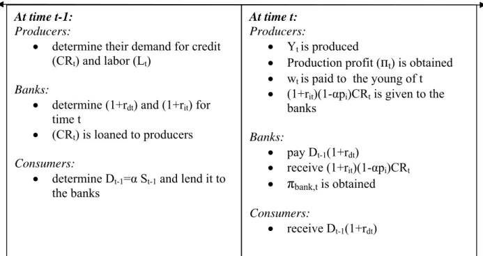
+ to the consumers who have supplied the deposits. These events can also be seen from Table 1.

At time t-1:

Table 1: Timing of Events

Producers:

• determine their demand for credit (CRt) and labor (Lt)

Banks:

• determine (1+rdt) and (1+rit) for

time t

• (CRt) is loaned to producers

Consumers:

• determine Dt-1=α St-1 and lend it to

the banks

At time t:

Producers:

• Yt is produced

• Production profit (

п

t) is obtained

• wt is paid to the young of t

• (1+rit)(1-αpi)CRt is given to the banks Banks: • pay Dt-1(1+rdt) • receive (1+rit)(1-αpi)CRt •

π

bank,t is obtained Consumers: • receive Dt-1(1+rdt)

(39)

III.3 Modeling Bank Regulation and Supervision

This section considers consumers’ producers’ and banks’ problem in an OLG framework. In subsection III.3.1, we consider the case where all producers are identical and credit conversion ratio depends only onα ; and in III.3.2, all producers are heterogeneous, implying different moral hazard rates.

III.3.1 Homogenous Producers

Consumer’s Problem:

Consumer maximizes its two period log utility function by choosing their two period consumption levels for a given time preference indicator, ρ . The consumer either saves (s) or consumes (c) its first period income, which is composed of wages (w) and profits from production Y_t₋₁7 ccordingly, the amount saved in the first period will also

be obtained. . A 1 Maximize t c− 1 ln( ) ln( ) 1 t -1 t c ρ + + c (1.1) subject to s_t-1+c_t-1≤w_t-1+ −(1 α)cr_t-1 (1.2) where we define cr CR L

= , which is defined as credit per labor.

7_{Profit from production is essentially unused credit}₍₁₋_α_)cr_{as will be shown below in the producer’s}

(40)

Consumer deposits α portion of its savings into the banks (that is, d_{t 1}− =αs_t-1),

and receives the return of (1+r_dt) in the next period. Hence, second period constraint is:

(1 ) (1 )

t t-1 dt

c ≤αs +r + −α s_t-1 (1.3)

Inserting s_t-1=w_t-1+ −(1 α)cr_t-1−c_t-1 from equation(1.2), into inequality(1.3), and

considering that equalities hold, we obtain

( (1 ) )( (1 ) (1

t

t t -1 t -1 t -1 d

c = w + −α cr −c α +r + −α))

when solved for w_t-1+ −(1 α)cr_t-1(income flow of consumers), this indicates:

(1 ) (1 ) (1 ) t t t -1 t -1 t -1 d c w cr c r α α α + − = + + + − (1.4)

The Lagrangian of this optimization problem using the objective function (1.1) and the above constraint (1.4) is:

1 ln( ) ln( ) ( (1 ) ( )) 1 (1 t t -1 t t -1 t -1 t dt c L c c w cr c r λ α ρ = + + + − − + + + )α + −(1 α) (1.5)

where

λ

is the Lagrange multiplier. The first order conditions (FOC) yield:

1 t -1 c =λ (1.6) and 1 1 1 1 ρ c_t λ (1 r_dt)α (1 α) ⎛ ⎞ ⎛ ⎞ = ⎜ ⎜ ₊ ⎟ ₊ ₊ ⎝ ⎠ ⎝ − ⎠⎟ (1.7)

(41)

whose solution together yields:

1 1 1 1 1 ρ c_t c_t-1 (1 r_dt)α (1 α) ⎛ ⎞ ⎛ ⎞ = _⎜ ⎜ ₊ ⎟ ₊ ₊ ⎝ ⎠ ⎝ − ⎠⎟ (1.8) or: (1 ) (1 ) 1 dt t -1 t r c α α c ρ ⎛ + + − ⎞ = ⎜ ₊ ⎟ ⎝ ⎠

When we use the equation (1.4) and write in terms of c_t c_t-1 the solution looks like:

(1 ) (1 ) 1 (1 ) 1 (1 ) (1 ) t dt t -1 t -1 t -1 t -1 d r c c w cr r α α _α ρ α α ⎛ ⎞ ⎛ + + − ⎞ + _⎜ _⎟⎜⎜ ⎟_⎟= + + + − ⎝ _⎠⎝ _⎠ + − and hence: 2 (1 ) 1 t -1 t -1 t -1 c ρ w α ρ ⎛ + ⎞₌ _{+ −} ⎜ ₊ ⎟ ⎝ ⎠ cr or: 1 ( (1 ) ) 2 t -1 t -1 t -1 w α cr ρ ρ ⎛ + ⎞ + − _⎜ _⎟= + ⎝ ⎠ c ) r

Thus, the ratio of savings to the first period income of the consumer (wt-1+ −(1 α)ct-1

is: 1 1 1 2 (2 ρ ) ρ ρ ⎛ + ⎞ −_⎜ _⎟= + + ⎝ ⎠

This implies that per consumer amount of deposits in the banks is:

1 1 ( (1 ) (2 ) t t -1 d α w ρ − = ₊ + −α crt -1) (1.9)

(42)

Hence, deposits will be affected by α , but not by ; since we have inelastic supply of deposits (with respect to ) and since is a cost for the bank it will pay 0 interest rate dt r dt r r_dt 8_. Producer’s Problem:

Producers maximize their profit (∏_prod) by choosing the optimal level of credit (CR) that will be borrowed from the bank, and the amount of labor that will be obtained from the consumers. In this setting, we assume that producers are homogenous in that they face the same level of credit interest, which is (1+ . Also, in this case, we assume r) that pi =1. The producer transfers to the consumer the (1−αpi) amount of credit that is

not used in the production process because of imperfections in the regulation and supervision process (See equation(1.2)).

Accordingly, the general profit function of the producer will be:

1 ₍₁ ₎

prod AK Lt t wLt Kt r

β −β

∏ = − − + (2.1)

where A denotes technology, L denotes labor, w denotes wages and capital ( )K_t follows

the process :

t t-1 t-1 t

K =K −δK +dK (2.2)

Since we assumed that the depreciation rate ( )δ is %100, we have:

t t t

K =dK = (2.3) I

(43)

Considering the model features:

t t i

K = =I αp CR (2.4)

Putting equation (2.4) in the production function in equation (2.1), we obtain: Maximize CR,L 1 (1 ) prod A p CR Li t t w Lt t p CRi t r β β β β α − α ∏ = − − + (2.5)

We assume A=1 and p_i = and accordingly, we stop using these terms in the 1

following.

The FOCs are as follows9:

1 1 ₍₁ _{) 0} prod CR L r CR β β β α β − − α ∂ ∏ = − + = ∂ which implies: 1 1 ( 1 ) 1 L r CR β β β β α − − − = + (2.6)

For the purpose of simplicity we denote credit per labor as: cr CR L = . Then, (2.6) becomes: 1 (1 ) ( cr) β r β α − = + (2.7)

After some manipulation of Equation (2.7) the demand for credit (in per capita terms) is: 1 1 1 1 cr r β β α − ⎛ ⎞ = ⎜ ₊ ⎟ ⎝ ⎠ (2.8) Also, given:

9_{From now on we will not use the time indicator since we consider each variable at time t except}

1

t

d₋

(44)

(1 ) 0 prod CR L w L β β β α β − ∂ ∏ = − − ∂ = one obtains: (αcr) (1β −β)= (2.9) w

Equation (2.9) implies that wages increase both with the level of credit extended to the producers, and with α.

Bank’s Problem:

The bank determines the level of (1+ and (1r) +r_d)that maximizes its profit

. Here credit and deposit are referred to as per capita values:

(∏_bank) cr CR L = and D d L

= . So the bank’s aim is to maximize its profit with respect to each producer (π_bank).

we write the objective function as: When Maximize d (1+r ),(1+r) πbank = +(1 r)αcr− +(1 r dd) t−1 (3.1) subject to cr≤d_t−₁ (3.2)

From equation (1.9) we know that consumers have inelastic supply of deposits. Since there are no investment alternatives for consumers, the only thing they can do is to keep their savings in bank regardless of the rate of return. This means that consumers will accept any interest rate on their deposits if it is more than or equal to 0. Hence, it is optimal for banks to set r_d =0.

(45)

In order to determine the credit interest, (1+ , bank uses equation(2.8), per r) capita credit demand of producers.

When we insert (2.8) in the equation (3.1) and take (3.2) as equality we obtain:

1 1 1 1 1 (1 ) 1 1 bank r r r 1 β β β β π α α α − − ⎛ ⎞ ⎛ ⎞ = + _⎜ _⎟ − _⎜ _⎟ + + ⎝ ⎠ ⎝ ⎠ (3.3)

which is simplified as:

1 1 1 ((1 ) 1) 1 bank r r β β π α − ⎛ ⎞ _α = _⎜ _⎟ + − + ⎝ ⎠ (3.4)

Here we have to make additional assumption so that we have non-negative profit function10:

(1+r)α≥ (3.5) 1

Then FOC of this problem is:

1 1-2 1 ( (1 ) 1) 0 (1 ) ( 1)(1 ) bank r r r β β β π β βα α β − − ∂ ₌ + − ₌ ∂ + − + (3.6) Accordingly; 1 (1 r) βα + = (3.7)

Given interest rate (3.7) corresponding credit demand will be: 1 2 1 ( ) supply demand cr =cr = β αβ −β (3.8)

10_{For concavity of the function we must have}

1 3 2 1 1 2 (1 ) ( 2 (1 )) 0 ( 1) r r β β β _β _β _βα β α − − − + − + + ≤ − ⎡ ⎤ ⎢ ⎥ ⎢ ⎥ ⎣ ⎦ which implies β ≤1.

(46)

Profit per producer will be:

1 2 1 1 ( 1)( ) bank β β π β α β − = − (3.9)

From these results we see that when α increases, the interest rate imposed on producers will be lower leading to increase in the credit demand. Accordingly, we can say that the greater the RS, the more credit will be demanded by the firms. We next turn to the case of non-homogenous producers.

III.3.2 Non-Homogenous Producers

In this setting we have heterogeneous producers denoted by , where is between 0 and 1 to indicate proportions of credit that is put into investment. In this setting, we have the same consumer’s problem except the consumer budget

i

p p_i

11_{, but we}

have to modify the producer’s and bank’s problem. So, for the consumer’s problem one can go back to the equations (1.1) through(1.9).

Producer’s Problem:

In this setting since producers (i=1 to n) are heterogeneous they will demand different levels of credit and labor as they will also pay different levels of interest. Hence the problem of producer i becomes:

CR,L

Maximize ∏_{prod i}_, =(αp CR_i _i)βL_i1−β −wL_i− +(1 r_i)(αp CR_i _i) (4.1)

)

r r )

11_{Now we will use the budget}₍ ₍₁ ₎ _{instead of}₍ ₍

t -1 i t -1

(47)

Here we have values that are uniformly distributed over the interval [0,1] p_i

The FOCs of the producer’s problem are the following:

, ₍ ₎ 1 1 ₍₁ ₎ prod i i i i i i p CR L p CR β β β α β − − α ∂ ∏ 0 = + − = ∂ which is solved for cr as:

1 1 ( ) (1 ) ( ) i i cr r p β β i β α − − = + (4.2)

Accordingly, producer i’s demand for per capita credit is : 1 1 1 1 i i cr p r β β α − ⎛ ⎞ = _⎜ _⎟ + ⎝ ⎠ (4.3) Also, , ₍ _{) (1} ₎ prod i i p CR L w L β β β α β − ∂ ∏ 0 = − − ∂ =

when simplified using cr CR L

= yields:

( p cri i) (1 ) w

β

α −β = (4.4)

From equation (4.4) it can be seen that, as different from the earlier solution, wages also increase in . p_i

Bank’s Problem:

Bank will again determine the level of (1+ and (1r) +r_d) that will maximize the

bank’s profit. But now, facing the potential moral hazard problem, bank has two options: to monitor the producers and give individualized interest rates and credit or, not to

(48)

monitor them and give uniform interest rates and credit. These cases will be considered in subsections III.3.2.1 and III.3.2.2 respectively.

III.3.2.1 Monitoring

In this case, bank may monitor producers and gives individualized interest rates. This option will be analyzed with respect to two alternatives: when the monitoring costs are fixed and when they are variable.

i) Variable Monitoring Cost:

Bank has a monitoring cost of ( )γ α per unit of per capita credit given to the producer. ( )γ α is a negative function of α so that when α increases monitoring costs decrease. In this case, profit maximization problem of the bank will be:

Maximize (1 ) (1 ( )) ₁ d i bank i i i d t (1+r ),(1+r ) π = +r αp cr− + +r γ α d− (5.1) ₁ i t subject to cr ≤d− (5.2)

From equation (1.9), we know that consumers have inelastic supply of deposits and thus, is zero. In order to determine (1r_d + for each producer, we write in r_i)

terms of from equation (4.3), and use the constraint in equation (5.2). From the first order conditions the profit maximizing level of interest rate is found to be:

i cr (1+r_i) 1 ( ) (1 _i) i r p γ α βα + + = (5.3)

(49)

Then from the equation (4.2) the optimal level of credit will be (given the interest rate by banks): 1 2₍ ₎ ₁ 1 ( ) i i p cr β _β β α γ α − ⎛ = ⎜ ₊ ⎝ ⎠ ⎞ ⎟ (5.4)

ii) Fixed Monitoring Cost:

In this setting, monitoring cost ( ( )ψ α ) is a fixed amount per producer (but still a negative function ofα ), then corresponding optimization problem will be:

Maximize

d i

(1+r ),(1+r ) πbank = +(1 ri)αp cri i− +(1 r dd) t−1−ψ α( ) (5.5)

subject to cr_i ≤d_t₋₁ (5.6)

Similar to the case of homogenous producers, the optimal level of interest rate will be:

1 (1 i) i r p βα + = (5.7)

Following the steps in the earlier case (i), optimal level of credit is found to be: 1 2 1 ( i i cr = β αβpβ)−β (5.8) III.3.2.2 No Monitoring

In this case, bank gives a uniform interest rate and credit to each producer, where expected type of the producer is the mean of the distribution, that is assuming that producer types are uniformly distributed on [0,1] the expected will be 0.5.

i

p = 0.5

i

(50)

When α is too low leading to high monitoring cost, bank may choose to give the same interest rate to each producer since it is too costly to determine the type of each consumer. In this case, the interest rate will be the rate that maximizes the following profit function: Maximize d i (1+r ),(1+r ) πbank = +(1 ri)αp cri i− +(1 r dd) t−1 (5.9) subject to cr_i ≤d_t₋₁ (5.10) As before 1+ =r_d 1.

In this profit function we do not have the monitoring cost. When we write with respect to (1 from the equation (4.2) and the FOC is:

i cr ) i r + 2 (1 r) βα + = (5.11)

From equation (4.3) the optimal level of credit (given the interest in(5.11)) will be: 2 1 _{( )}1 2 cr β β α β β − − = (5.12)

III.4 Profit Calculation

Now, we consider the conditions under which conditions monitoring is more profitable for the bank. In order to examine this, we will calculate the profit of the bank in cases of fixed monitoring cost, variable monitoring cost and no monitoring cost respectively in subsections III.4.1, III.4.2 and III.4.3.

(51)

III.4.1 Fixed Monitoring Cost

If the bank has fixed monitoring cost per producer monitored, inserting the optimal level of credit and interest (Equations (5.7) and (5.8)) , in equation (5.5), the level of profit per producer is found as:

1 2 2 1 1 1 1 ( )( ( ) ) ( ) ( bank i i i i p p p p β β β β β ₎ π β α α β α ψ α βα − − − = − −

which can be simplified as:

1 2 1 1 ( 1)( ( ) ) ( bank pi β β ₎ π β α ψ α β − = − − (6.1)

Hence bank’s profit only depends on α andβ. If we write the total profit function of the bank:

( ) bank pi d i β β β α ψ α β 1 1 2 1− 0 ⎛ ₁ ⎞ ∏ = ⎜_⎜( −1)( ( ) ) − ⎟_⎟ ⎝ ⎠

∫

p

If we solve for the integral, corresponding total profit will be:

( ) bank β β β α β ψ β 1 2 1− 1 ∏ = ( −1)( ) (1− ) − α (6.2)

III.4.2 Variable Monitoring Cost

If the bank has variable monitoring cost per unit of credit borrowed, inserting equations (5.3) and (5.4), in equation (5.1) we find the corresponding profit level per producer as:

(52)

1 1 1 1 2₍ ₎ 2₍ ₎ 1 ( ) (1 ( )) 1 ( ) 1 ( ) i i bank i i p p p p β β β β β α β α γ α π α γ α βα γ α γ α − − ⎛ + ⎞ ⎛ ⎞ ⎛ ⎞ =_⎜ _⎟ _⎜ _⎟ − + _⎜ _⎟ + + ⎝ ⎠ ⎝ ⎠ ⎝ ⎠

which is simplified as:

1 2₍ ₎ ₁ 1 ( 1) (1 ( )) i bank p β β β β α π β γ α − ⎛ ⎞ = _{− ⎜} + ⎝ ⎠⎟ (6.3)

If we write the total profit function of the bank:

i bank i p dp β _β β β α β γ α 1 1 2 ₁₋ 0 ⎛ ⎞ ⎛ ( ) ⎞ 1 ⎜ ⎟ ∏ = _⎜_{( −1)⎜} _⎟ _⎟ (1+ ( )) ⎝ ⎠ ⎜ ⎟ ⎝ ⎠

∫

If we solve for the integral, corresponding total profit will be:

bank β _β β β α _β β γ α 1 2 ₁₋ ⎛ ⎞ 1 ∏ = ( −1)_⎜ _⎟ (1− ) (1+ ( )) ⎝ ⎠ (6.4) III.4.3 No Monitoring

Bank gives uniquely determined interest rate and credit that is determined under the assumption that the expected p_i ( e)

i

p is equal to 0.5. Accordingly, the credit interest

and credit supply are (1 r) 2

βα + = and 2 1 _{( )}1 2 supply cr β β α β β − − = respectively.

If we calculate the optimal levels of credit for the producers (credit demand denoted by cr_demand) for p_i <0.5 and p_i >0.5 and compare this with crsupply :

(53)

1 2 ₁ 1 1 1 1 ( ) 2 2 2 supply cr β _β β β β α β β α βα − − − − = = ⎛ ⎞ ⎜ ⎟ ⎝ ⎠ (6.5)

(

)

( )

1 2 1 , 1 1 1 2 demand i i cr p β _β β β α − − = (6.6) Accordingly:

For p_i >0.5, cr_demand <cr_supply For p_i<0.5, cr_demand >cr_supply

so that the agents with will not use the credit for production since given credit is not enough to obtain the optimal level of profit which is indeed zero in case of perfect competition. This means that producers, who would incur negative profit when they transform all of the credit into production, naturally choose not to use this credit for production and they rather consume it. Conversely producers with will use only the optimal amount of credit for production and consume the rest. Hence, both groups’ optimal behavior exhibits moral hazard.

0.5 i p < 0.5 i p >

Along with the explanation above, profit function of the bank in non-monitoring case will be:

bank pi pi pi i β β β β β β α β α β α αβ 2 2 1 1− 1− 1− 1− 0.5 ⎛ ₂ ⎞ ∏ = ⎜_⎜ ( ) − ( ) ⎟_⎟ ⎝ ⎠

∫

dp Then:

(54)

1 2 2 1 1 1 1 1 1 1-= 2 (1- 2 ) (1 )(1 2 ) 2 bank β β β β 1 β β β β β β β α β α β β + − − − − − − − ⎛ ⎞ ∏ _⎜ _⎟ − − ⎝ ⎠ β − − −

In a more simplified version:

= bank β β β β β β β β β α β β 1+ −2 −1 1− 1− ⎡ 2 1− 1− ⎤ ∏ (1− ) ⎢ (1− 2 ) − (1− 2 )⎥ 2 − ⎢ ⎥ ⎣ ⎦ (6.7)

III.5 Bank’s Decision Process

In this section we will compare the profits for each case of monitoring calculated in section III.412. The following profit functions (6.8), (6.9) and (6.10) correspond to the fixed-cost, variable-cost and no monitoring cases, respectively:

Fixed-cost monitoring (from equation (6.2)):

(

2

)

₁1 1 = ( 1) (1 ) ( ) bank β _β β α β ψ β − ∏ − − − α (6.8)

Variable-cost monitoring (from equation (6.4)):

1 2 ₁ 1 = ( 1)(1 ) (1 ( )) bank β _β β β α β β γ α − ⎛ ∏ − − _{⎜ +} ⎝ ⎠ ⎞ ⎟ (6.9)

No monitoring (from equation (6.7)):

= bank β β β β β β β β β α β β 1+ −2 −1 1− 1− ⎡ 2 1− 1− ⎤ ∏ (1− ) ⎢ (1− 2 ) − (1− 2 )⎥ 2 − ⎢ ⎥ ⎣ ⎦ (6.10)

12_{Here we have two terms indicating different kinds of monitoring costs.}_{θ α}_{( )}_{is used for fixed}

(55)

In the following, we will simulate each of these profit functions using some reasonable values of α and β, and assuming appropriate fixed and variable cost functions. Fixed monitoring cost ( ( )ψ α ) is assumed to be fixed proportion ( ( )θ α ) of expected per capita income and variable monitoring cost is assumed to be a negative function of α .

Accordingly, cost functions are given as: ( ) ( )Y

L ψ α θ α − = and θ α( ) γ α( ) 1 α = = . 13 For α , we take the range between 0 and 1.

III.5.1 Fixed Cost versus Variable Cost

We have the following relationship between ( )θ α and ( )γ α if we equalize profits for fixed and variable monitoring costs in equations (6.8) and (6.9):

(

)

1 1 2 ₁ 1 1 ( 1)(1 ) 1 ( ) 1 ( ) Y L β β β _β β β α θ α β γ α − − − ⎛ ⎞ ⎛ ⎞ ⎜ ⎟ − − _⎜ −_⎜ _⎟ _⎟= + ⎝ ⎠ ⎜ ⎟ ⎝ ⎠

Provided that the following condition holds (ie. equation (6.8) - (6.9) ≥0):

(

)

1 1 2 ₁ 1 1 ( 1)(1 ) 1 ( ) 1 ( ) Y L β β β _β β β α θ α β γ α − − − ⎛ _⎛ _⎞ ⎞ ⎜ ⎟ − − _⎜ −_⎜ _⎟ _⎟− ≥ + ⎝ ⎠ ⎜ ⎟ ⎝ ⎠ 0 (6.11)

bank’s profit in case of fixed monitoring cost will be greater than the profit in case of variable monitoring cost. Simulation analysis reported in the Appendix reveals that this condition is never met for β < 0.5 that are indeed suggested by Mankiw et al. (1992) to

13_{Considering expected per capita income as}

( )

₍

i i Y p p L β β _β _β _β α β α2 1− −

= ) corresponding fixed monitoring

cost becomes ( ) 2 1 2 1 1 1 i p β β β β β β ψ α α₌ −−β − −

(56)

be the feasible values for β14. This indicates that incurring variable monitoring cost is always preferred by profit maximizing banks.

III.5.2 Fixed Cost versus No Monitoring

The following is the condition under which bank profits under fixed monitoring cost is higher than those under no monitoring (ie. equation (6.8) - (6.10) ≥0)

( )Y L β β β β β β β β β α β β θ α β − 1+ −2 −1 1− 1− ⎡ 2 1− 1− ⎤ (1− ) ⎢(1− ) − (1− 2 ) + (1− 2 ) −⎥ ≥ 0 2 − ⎢ ⎥ ⎣ ⎦

If we simplify this inequality further, we find the following relationship between α and

β: ( )Y L β β β β β β θ α β β β β β β α − 1+ −2 −1 1− 1− 1− 1− ⎡ ₂ ⎤ ≤ (1− ) ⎢(1− ) − (1− 2 ) + (1− 2 )⎥ 2 − ⎢ ⎥ ⎣ ⎦ (6.12)

Simulation analysis in Appendix shows that that this condition is never met for the feasible β values . This means that monitoring producers with fixed monitoring cost is never profitable for the bank as compared to not monitoring them.

III.5.3 Variable Cost versus No Monitoring

If we examine the condition under which monitoring with variable cost is more profitable for the bank we find (ie. equation (6.9)-(6.10)≥0):