EVALUATION OF ARMY CORPS FOOD SUPPLY SYSTEM
USING SIMULATION
A THESIS
SUBMITTED TO THE DEPARTMENT OF INDUSTRIAL ENGINEERING
AND THE INSTITUTE OF ENGINEERING AND SCIENCES OF BILKENT UNIVERSITY
IN PARTIAL FULFILLMENT OF THE REQUIREMENTS FOR THE DEGREE OF
MASTER OF SCIENCE
BY
OZAN PEMBE
July, 2002
I certify that I have read this thesis and in my opinion it is fully adequate, in scope and in quality, as a thesis for the degree of Master of Science.
Assoc. Prof. İhsan Sabuncuoğlu (Principal Advisor)
I certify that I have read this thesis and in my opinion it is fully adequate, in scope and in quality, as a thesis for the degree of Master of Science.
Assoc. Prof. Erdal Erel
I certify that I have read this thesis and in my opinion it is fully adequate, in scope and in quality, as a thesis for the degree of Master of Science.
Asst. Prof. Oya Ekin Karaşan
Approved for the Institute of Engineering and Science
Prof. Mehmet Baray
ABSTRACT
EVALUATION OF ARMY CORPS FOOD SUPPLY SYSTEM
USING SIMULATION
Ozan Pembe
M.S. in Industrial Engineering
Supervisor: Assoc. Prof. İhsan Sabuncuoğlu
July, 2002
Food Supply System is one of the main elements of Army Logistics System. The ultimate objective in food supply system is to provide the food at the right time and at the right place. If this objective is achieved, the morale, the health and the strength of the soldiers on the battlefield will enormously enhance.
In the literature, particularly in Turkish Army, there is no study which tests whether the existing food supply system operates properly or not under the war conditions and which shows the potential problem areas and which specify time standards under different scenarios. The objective of this study is to answer these questions by the help of simulation model of the system. This model can also be helpful to the staff officers who prepare logistic support plans.
The simulation model of Army Corps Food Supply System is built in Arena 3.0. The results are analyzed by statistical methods. The related bibliography is also provided in the thesis.
Key Words: Military Simulation, Food Supply System, Logistics, Class I Supply
ÖZET
SİMULASYONLA BİR KOLORDUNUN ERZAK İKMAL
SİSTEMİNİN ANALİZ EDİLMESİ
Ozan Pembe
Endüstri Mühendisliği Bölümü Yüksek Lisans
Danışman: Doç. İhsan SABUNCUOĞLU
July, 2002
Erzak ikmal sistemi Türk Silahlı Kuvvetleri ikmal sisteminin ana parçalarından biridir. Erzak ikmal sistemindeki nihai amaç erzağın istenilen yer ve zamanda hazır bulundurulmasıdır. Bu amaç gerçekleştiğinde muharebe sahasındaki askerin sağlığı, morali ve gücü artacaktır.
Literatürde şu ana kadar mevcut sistemin muharebe şartlarında uygun çalışıp çalışmadığını test eden, problem sahalarının neler olduğunu gösteren ve farklı senaryolar altında bu sisteme ait zaman standartlarının tespit edildiği bir çalışma yapılmamıştır. Bu tezde biz mevcut erzak ikmal sisteminin simulasyon modelini kurarak bu soruları cevaplamaya çalıştık. Ayrıca bu çalışmanın lojistik destek planlarını hazırlayan karargah subaylarına yardımcı olacağını düşünüyoruz.
Sistemin simülasyon modeli Arena 3.0 kullanılarak geliştirildi. Neticeler istatistiksel metodlar kullanılarak incelenmiştir. İlgili literatür de bu tezde sunulmuş bulunmaktadır.
Anahtar Kelimeler: Askeri Simülasyon, Erzak İkmal Sistemi, Lojistik, I.Sınıf İkmal
ACKNOWLEDGEMENT
I would like to express my deep gratitude to Dr. İhsan Sabuncuoğlu for his guidance, attention, understanding, and patience throughout all this work.
I am indebted to the readers Dr. Erdal Erel and Dr. Oya Ekin Karaşan for their effort, kindness and time.
I would like to thank all Industrial Engineering Faculty staff and my friends for their support and encouragement.
CONTENTS
1. Introduction
1.1. Logistic Activities In Army... 1.2. Supply Concept In Army... 1.2.1. Levels of Supply... 1.2.2. Classes of Supply Material ... 1.2.3. Food Supply System In Army Corps...
2. Literature Review
2.1. Simulation Software and Methodology... 2.2. Military Simulation... 2.3. Military Logistics...
3. The Simulation Model
3.1. Formulation of the Problem and Planning the Study... 3.2. Model Development... 3.2.1. Conceptual Model... 3.2.2. Logical Model... 3.2.3. Simulation Model (Computer Code)... 3.3. Input Data Analysis... 3.4. Model Verification and Validation... 3.4.1. Verification... 3.4.2. Validation... 3.4.2.1. Face Validity... 1 1 2 3 4 5 9 9 11 12 14 14 15 16 19 23 24 25 25 27 27
3.4.2.2. Sensitivity Analysis...
4. Design and Analysis of Experiments
4.1. 2k Factorial Designs... 4.2. Diagnostic Checking on The Validity of Assumptions... 4.3. Evaluation of Main Effects and Interactions for Maximum
Time-In-System Performance Measure ... 4.4. Evaluation of Main Effects and Interactions for
Number-of-destroyed-vehicles Performance Measure... 4.5. Sensitivity Analysis... 4.6. Conclusion……….
5. Implementation of Analytic Hierarchy Process for Army Corps Food Supply System
5.1. Introduction... 5.2. Implementation of AHP... 5.2.1. Calculation of Maximum Eigen Value and Eigenvectors... 5.2.2. Consistency Checking ... 5.2.3. Synthesis...
6. Conclusions
6.1. General... 6.2. Concluding Remarks and Future Research Topics...
27 29 29 31 37 42 44 46 48 48 50 53 55 56 58 58 59
APPENDICES
A. Main Units in The Organization of An Army Corps... B. A Small Part From Computer Code... C. The Application of Sequential Process... D. The Outputs of Treatments for Each Performance Measure... E. Regression Models of the Performance Measures... F.Residual Analysis of Performance Measures... G. The ANOVA Results of Performance Measures... H. The Output of One Replication From The Simulation Model... I. Flowchart Model of The System ... BIBLIOGRAPHY... 61 62 64 65 69 70 72 75 78 88
List of Figures
1.1. Food Supply System of Army Corps... 1.2. The Flow of Distribution and Requisition... 3.1. Schematic View of The Model Development... 3.2. The Flowchart Model of Activities During Traveling ... 3.3. The Flowchart Model of Loading Activities... 3.4. A Screen Shot from The Animation of The Model... 3.5. Sensitivity Analysis on the Loading Times... 3.6. Organization of An Army Corps... 3.7. Detailed Flowchart Model of The System... 4.1. Scatter Plot of Variances for Number of Destroyed Vehicles... 4.2. Scatter Plot of Residuals for Number of Destroyed Vehicles... 4.3. Main Effects of Significant Factors for MTIS... 4.4. The Interaction Effect Between Factor A and Factor B for MTIS... 4.5. The Interaction Effect Between Factor A and Factor C for MTIS... 4.6. The Interaction Effect Between Factor A and Factor E for MTIS... 4.7. Main Effects of Significant Factors for Number of Dest. Vehicles... 4.8. The Interaction Effect Diagram of Factor C and Factor D...
6 8 16 21 22 26 28 61 78 36 36 37 39 40 41 42 43
List of Tables
2.1. Summary Table of Related Literature... 3.1. Technical Information About The Model... 3.2. Repair Times of Vehicles ... 3.3. Hit and Kill Probabilities of Enemy Weapons... 3.4. Loading and Unloading Times of Vehicles... 3.5. Points of Experiment for The Sensitivity Analysis on Loading Times... 4.1. Description and Levels of Factors... 4.2. The Results of Kolmogorov-Smirnov and Anderson-Darling Tests... 4.3. Result Of Bartlett Test for MTIS... 4.4. Result of Bartlett Test for MTIS (Transformed Data)... 4.5. Significant Factors and Interactions for Performance Measures... 4.6. Sensitivity Analysis (I)……….. 4.7. Sensitivity Analysis (II)……… 4.8. Summary Table for The Application of Sequential Procedure for MTIS... 4.9. Summary Table for Application of S.P. for The Number of
Destroyed Vehicles...……... 4.10. Data Set Of 32 Treatments for MTIS... 4.11. Data Set Of 32 Treatments for Number of Destroyed Vehicles... 4.12. Regression Models... 4.13. Residuals for the Maximum Time in System Performance Measure... 4.14. Residuals for The Number of Destroyed Vehicles...
10 23 24 24 24 28 31 32 33 34 45 46 47 64 64 65 67 69 70 71
4.16. Analysis of Variance for Maximum Time in System
(Transformed Data)...………... 4.17. Analysis of Variance for The Number of Destroyed Vehicles... 5.1. Alternative Designs for The Army Corps Food Supply System... 5.2. Mean Values of MTIS for Four Alternatives... 5.3. Subjective AHP Scale... 5.4. Preference Matrix of Alternatives for MTIS Criteria (Matrix-A)... 5.5. Preference Matrix of Alternatives for CCC Criteria (Matrix-B)... 5.6. Preference Matrix of Alternatives for VEA Criteria (Matrix-C)... 5.7. Preference Matrix of Three Criteria (Matrix-D)... 5.8. Maximum Eigen Values and Eigenvector of Weights of Matrices... 5.9. AHP Consistency Limits... 5.10. The Consistency Index Values of Matrices... 5.11. Relative Performance of Each Alternative...
73 74 48 49 50 51 52 52 52 54 55 56 56
Chapter 1
Introduction
1.1. Logistic Activities in Army
Logistics means having the right thing, at the right place, at the right time. In its most comprehensive sense, it includes all the following activities;
• Design and development, acquisition, storage, transport, distribution, maintenance, evacuation, and disposition of materials.
• Transport of personnel.
• Acquisition or construction, maintenance, operation and disposition of facilities.
• Acquisition or furnishing of services • Medical and health service support.
The goal of logistics is to provide the support required to ensure that operations succeed. The main task of logistics in Turkish Army is to provide logistic support to Turkish Army Forces at all levels of war. A dependable uninterrupted logistics system helps commanders seize and maintain the initiative. Thus, logistic planning should be executed as an integral part of force and operational planning. During the planning process of logistic support, the principles below are used as a guiding tool :
• Standardization: Methods used in logistic systems and in its sub-systems, services and materials should be standardized. Hence, this will enhance the operational effectiveness of armed forces.
• Sufficiency: Levels and distribution of logistic resources must be sufficient to achieve designated levels of readiness, sustainability and mobility to provide the required military capability during peace, crisis and conflict.
• Flexibility: Logistic Support must be as dynamic, flexible, mobile and responsive as the operational formations.
• Simplicity: This principle has a contribution to increase the effectiveness in planning process of logistic support. Anticipation of requirements for any kind of military operation and allocation of resources can be made easier if simplicity in logistic planning is provided.
• Visibility: For an efficient management of logistics system, the number, situation and activities of support units in this system should be visible in electronic environment.
• Responsibility and authority of logistic support units, and sections should be determined elaborately.
• Cooperation and coordination
• Economy: Logistic resources must be used effectively, efficiently and economically.
1.2. Supply Concept in Army
Supply is a wide-ranging function that extends from determination of requirements at the national level down to delivery of items to the user in the theater. It involves activities at all levels of logistics. Supplying the force is one of the major elements in sustaining the battle. It is the process of providing all items necessary to equip,
maintain, and operate a unit. Supply operations involve the storage, distribution, requisitioning, protection, maintenance, and salvage of supplies. Its primary purpose is to sustain the soldiers and weapon systems in strategic, operational, and tactical environments on the modern battlefield. As the battle progresses, logistic support units must provide the right supplies at the right locations in time to contribute to the fight. It is imperative that the systems be in place to allow the supported units to place their demands rapidly and to assist the logistic support units in providing the supplies in a timely manner.
To be successful, supply support must be both effective and efficient. Limited resources require that supply operations be efficient. However, efficiency cannot handicap effectiveness. Five logistics characteristics facilitate effective, efficient supply operations. Foremost among these is anticipation. Commanders and logistician must anticipate requirements, and the supply system must also be anticipatory. They integrate supply concepts and operations with strategic, operational, and tactical plans. Supply operations and systems must be responsive to the commander and provide continuous support to forward-deployed forces. Finally, logistician must improvise to expedite actions when needed and adapt to changing dynamics on the battlefield.
1.2.1. Levels of Supply
Levels of supply are broadly classified under the categories of tactical, operational, and strategic.
Strategic level of supply: Strategic-level supply is involved with mobilization, acquisition, force projection, mobility, and the concentration of supply support in the
theater. It is the link between the nation's economic base and the military supply operations in a theater. Strategic and operational levels interface in a theater of operations.
Tactical level of supply: Tactical-level supply focuses on readiness. It supports the tactical commander’s ability to fight battles and engagements. Successful support is anticipatory. It provides the right supplies at the right time and place to supported units. Tactical commanders must integrate supply support with their concept of operations during the tactical planning phase. Mobile, responsive capabilities are essential for accomplishing the supply mission.
Operational level of supply: Operational-level supply focuses on sustainment, supply unit deployment, and the distribution and management of supplies and material. Contractors and civilians provide support from within as well as outside the theater of operations.
1.2.2. Classes of Supply Materials
Supply includes a broad assortment of items categorized in 5 classes. • Class I: Food , water, health and comfort items.
• Class II: Clothing, individual equipment, maps chemical defense equipment. • Class III: Petroleum fuels, lubricants, hydraulic and insulating oils, coal. • Class IV: Special purpose materials. For example cold-weather equipment. • Class V: Ammunition of all types, bombs, explosives, mines, fuzes, missiles, rockets and other associated items.
1.2.3. Food Supply System in Army Corps
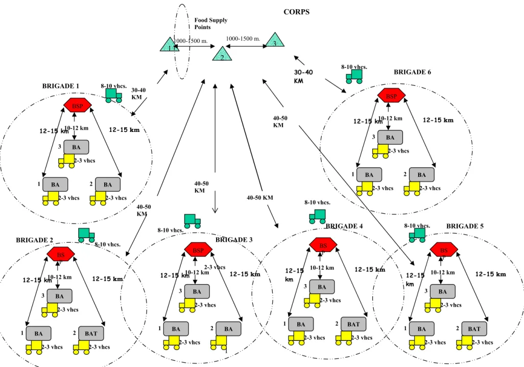
Request and distribution are two major components of food supply system. These activities are presented in Figure 1.1. In the system modeled in this study, Battalion Personnel Officer takes the number of soldiers in each company from the noncommissioned officer of the companies. Then the total number of soldiers in battalion is found and reported to the Personnel Office Administrator (POA) in the Brigade. The POA gives the total number of Brigade to the Quartermaster Office Administrator. Daily Ratio Demand of Brigade is prepared according to this total number. DRD shows the needed food of Brigade for the following day of operation. Then a convoy which consists of 8-10 vehicles is formed to get the needed subsistence of the brigade. This convoy starts its movement from Brigade Supply Point and may undergo different enemy attacks during its travel toward Corps Supply Point. When it arrives CSP, the convoy commander gives the requisition form which shows the Daily Ratio Demand of Brigade to the Food Supply Point Commander. FSPC orders loading section to load the convoy. After completion of loading each vehicle, convoy starts its travel back to Brigade Supply Point and may be attacked by enemy forces during its travel again. When convoy reaches BSP, the loading section in BSP unloads the vehicles. The food is then separated into piles. Each pile belongs to a specific battalion. This separation method is called unit pile method. Then each pile is again loaded upon the vehicles of Battalions, each battalion convoy which comprises 2 or 3 vehicles travels toward Battalion Regions under the threat of enemy attacks. When these convoys arrive at their regions, the mission is complete.
BSP BA BA BA 1 2 3 10-12 km 12-15 km 12-15 km 2-3 vhcs 2-3 vhcs 2-3 vhcs BRIGADE 1 BSP BA BA BA 1 2 3 10-12 km 12-15 km 12-15 km 2-3 vhcs 2-3 vhcs 2-3 vhcs BRIGADE 6 40-50 KM 40-50 KM 30-40 KM CORPS 1 2 3 1000-1500 m. 1000-1500 m. Food Supply Points 8-10 vhcs. BS P BAT BA BA 1 2 3 10-12 km 12-15 km 12-15 km 2-3 vhcs BRIGADE 5 8-10 vhcs. BS P BAT BA BA 1 2 3 10-12 km 12-15 km 12-15 km 2-3 vhcs BRIGADE 4 8-10 vhcs. 8-10 vhcs. BSP BA BA BA 1 2 3 10-12 km 12-15 km 12-15 km 2-3 vhcs 2-3 vhcs BRIGADE 3 8-10 vhcs. BS P BA 3 10-12 km 12-15 km 12-15 km 2-3 vhcs BRIGADE 2 8-10 vhcs. 30-40 KM 40-50 KM 40-50 KM Figure 1.1. Food Supply System of Army Corps
In the military organization that we modeled there are 6 brigades, which are supported by Corps Supply Point and each brigade has 3 battalions. There are 3 Food Supply Points in CSP and they are 1000-1500 meters away from each other. One of them is the main supplier and supports 2 brigades. The other two FSPs support 4 brigades but not always have the required amount of food in its depots. Figure 1.2 displays these activities.
Actually the reaction of this food supply system under war conditions is unknown since Turkish Army has not entered a full-scale war so far. By making simulation model of this system, we will be able to analyze the system and identify the problem areas. The model will also be a helpful tool for commanders in their decision-making process. Specification of time standards for this system under different scenarios is another useful outcome of this work. Because these standards will help staff officers prepare logistic plans efficiently and anticipate the duration of supply in FSS. A list of research questions to be answered by the proposed simulation study is given in Chapter 3.
Chapter organization is as follows. Chapter 2 presents the related literature with the simulation software and methods; the requirements of military simulation modeling; simulation applications that provide useful information about military logistics. In Chapter 3, we construct the simulation model of Army Corps Food Supply System and give a list of research questions to be answered by this simulation model. Chapter 4 presents experimental design of five factors; March technique, number of supply points, artillery attack, air attack, breakdown of vehicles. Moreover, we implement the ANOVA procedure to find out the significant factors for two different performance measures. Chapter 5 includes ranking and selection of the best alternative design by the
help of Analytic Hierarchy Process (AHP) technique. In Chapter 6, we give conclusions of our research and propose some ideas for future researches.
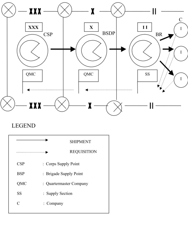
Figure 1.2. The Flow of Distribution and Requisition
X I I XXX SS QMC QMC I I I BSDP CSP BR C
LEGEND
REQUISITION SHIPMENTCSP : Corps Supply Point BSP : Brigade Supply Point QMC : Quartermaster Company
SS : Supply Section C : Company
Chapter 2
Literature Review
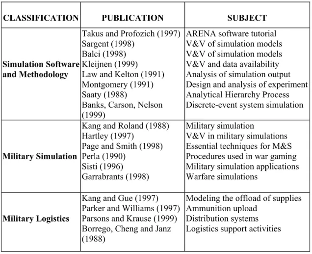
In this chapter, references are summarized in three sections. They are simulation software and methodology, military simulation, and military logistics. In the first section, we mention about the papers that helped us to build our simulation model and learn some techniques about verification and validation. In the second section, papers about military modeling and simulation are presented. In the last section, the papers about the distribution systems and logistic support activities in military environment are given. We summarized the related literature in Table 2.1.
2.1. Simulation Software and Methodology
In our study, we use ARENA 3.0 software to build the simulation model of Army Corps Food Supply System. Arena combines the modeling power and flexibility of the SIMAN simulation language, while offering the ease of use in Microsoft Windows and Microsoft NT environment. Takus and Profozich (1997) explain the software and its capabilities in their tutorial.
Sargent (1998) and Balci (1998) discuss how to assess the acceptability and credibility of simulation results, principles, and techniques of simulation validation, verification and testing. Kleijnen (1999) explains the statistical techniques to validate simulation models depending on the type of the data available. He explains three different cases as no data, only output data, both input and output data and gives some examples about them. Law and Kelton (1991) explain the timing and relationships of validation, verification and establishing credibility, and discuss guidelines for
Table 2.1. Summary Table of Related Literature
CLASSIFICATION PUBLICATION SUBJECT
Simulation Software and Methodology
Takus and Profozich (1997) Sargent (1998) Balci (1998) Kleijnen (1999) Law and Kelton (1991) Montgomery (1991) Saaty (1988)
Banks, Carson, Nelson (1999)
ARENA software tutorial V&V of simulation models V&V of simulation models V&V and data availability Analysis of simulation output Design and analysis of experiment Analytical Hierarchy Process Discrete-event system simulation
Military Simulation
Kang and Roland (1988) Hartley (1997) Page and Smith (1998) Perla (1990) Sisti (1996)
Garrabrants (1998)
Military simulation V&V in military simulations Essential techniques for M&S Procedures used in war gaming Military simulation applications Warfare simulations
Military Logistics
Kang and Gue (1997) Parker and Williams (1997) Parsons and Krause (1999) Borrego, Cheng and Janz (1988)
Modeling the offload of supplies Ammunition upload Distribution systems Logistics support activities
determining the level of model detail and some techniques for verification and validation.
Montgomery (1991) thoroughly discusses the design and analysis of experiments in his book. He introduces factorial designs, regression analysis, response surface methods and gives examples about them. Kelton (1997) introduces some of the ideas, issues, challenges, solutions, and opportunities in deciding how to experiment with a simulation model to learn about its behavior. Hood and Welch (1992) discuss experimental design issues in simulation.
Saaty (1988) presents Analytic Hierarchy Process (AHP), which works by developing priorities for alternatives and the criteria used to judge the alternatives. AHP provides a powerful tool that can be used to make decisions in situations involving multiple objectives. We choose AHP among many decision making methods because of its simplicity in both application and interaction with the decision makers.
2.2. Military Simulation
Kang and Roland (1988) discuss the military simulation within the subjects of organizations that deal with and their areas of study, classification of military simulation, simulation as a training tool, and application. They stress on the subjects of advanced distributed simulation, distributed interaction simulation, and high level architecture.
Hartley (1997) mainly stresses on the difficulties, methods, and cost of the military simulation studies and presents the comparison of military simulation studies with others in terms of verification, validation and accreditation.
Page and Smith (1998) provide an overview of military training simulation in the form of an introductory tutorial. Basic terminology is introduced, and current trends and research focusing on the military training simulation domain are described. Perla (1990) presents the art of war gaming, discussing the backbones of the procedures and techniques.
Sisti (1996) studies on the topics of interest to researchers in the simulation community and present some of the selected Air Force programs. He deals with the
wide variety of research issues in simulation science, and their application to the military domain.
Garrabrants (1998) stresses the role of simulation systems to support all levels of command and control functioning, especially staff planning after receipt of orders and mission rehearsal in his study. He explains how Marine Tactical Warfare Simulation, an advanced simulation system, is used to model all aspects of combat (air, land, sea, and amphibious ship-to-shore activities) and gives detailed information about its usage.
2.3. Military Logistics
Kang and Gue (1997) describe a simulation model of the offload of supplies to support a Marine Air-Ground Task Force, and show how to determine the number and allocation of different material handling devices for such an operation.
Parker and Williams (1997) prescribe a method for the strategic analyst to develop flow diagrams which can be used to analyze logistics requirements, project and evaluate force sustainment. They also evaluate the steady-state logistics flow of fuel and ammunition through time.
Parsons and Krause (1999) introduce the TloaDS simulation model that is a tool to study the delivery of logistics material to U.S. Marine Expeditionary Forces. This tool tries to provide inexpensive, flexible and frequent evaluation of new logistics delivery tactics and logistics material transport vehicles. It has purpose of encompassing all elements of the previously built models into one model, allowing for easy user modification increasing execution speed significantly.
Borrego, Cheng and Janz (1988) study on the Comprehensive Operational Support Evaluation Model for Space (COSEMS) which is a discrete event simulation with objective of evaluating alternative logistics support concepts that have been proposed by the Strategic Defense System (SDS). It is written in SIMSCRIPT II.5 and FORTRAN. The papers in military simulation part deal with the combat simulation and war gaming but the logistic support activities are not included in these papers whereas the papers in military logistic part just deal with the distribution systems and logistic support activities. In our study, we analyze both the effect of logistic support activities and enemy attacks.
Chapter 3
The Simulation Model
3.1. Formulation of The Problem And Planning The Study
In this study, we aim to explore the behavior of existing food supply system of Army Corps under war conditions, establish the nature of relationships among significant factors and the system performances, specify some time standards for the activities which occur within this supply system and compare different scenarios. In the case where the system does not work properly, we try to detect the major problem areas of the system. The following research questions will be investigated by the help of this model.• Does the existing food supply system of Army Corps operate properly ? • Does any bottleneck occur in the system ?
• How do artillery and air attacks of enemy affect the system performances ? • What happens if we change the organization of the facilities in the food supply
system ?
• What are the significant factors and how do they affect the system performance measures ?
• What kind of modifications can be made to improve the system performance measures of existing system ?
The performance measures under consideration are: • Maximum time in system (in minutes). • Number of destroyed vehicles.
The data requirements of our simulation model are: • The number of vehicles in a convoy.
• The velocity of the vehicles.
• Loading and unloading time of a vehicle. • Loading capacity of a food supply point.
• Repairing time of damaged vehicles by enemy attacks and usual breakdowns. • The hit and kill probabilities of enemy weapons.
The assumptions for our model are: • The basic unit is brigade.
• The organization of Army Corps is as in Appendix A.
• There are enough vehicles to carry the required food by the brigades. • There is enough food in Corps supply point.
• The operation under consideration is offense. • Air attack gun is 1 F-16 war plane.
• Artillery guns are 4 105mm. Cannons.
3.2. Model Development
In order to develop the simulation model, we first generate the conceptual model. During this process we consulted the officers in Logistics Information Systems Center. A schematic view of model development is given in Figure 3.1.
Figure 3.1. Schematic View of The Model Development
3.2.1. Conceptual Model
Conceptualizing a model is one of the important phases of model development. The real-world system under investigation is abstracted by a conceptual model. By the help of the conceptual model, we understand main structure of the system and focus on the essential components of the system. In our system the basic elements are:
Events :
• Departure of convoys from brigade supply points. • Artillery attack of enemy.
• Air attack of enemy.
• Occurrence of breakdowns because of enemy attacks. • Completion of repair of damaged vehicles event. • Arrival of convoys to Corps supply point.
• Loading event of the convoys. • Completion of loading event.
SIMULATION MODEL ASSUMED SYSTEM REAL WORLD CONCEPTUAL MODEL LOGICAL MODEL
• Departure of convoys from Corps supply point. • Arrival of convoys to brigade supply points. • Unloading event of vehicles.
• Arrival of convoys to Battalion Region.
Activities :
There are two main activities in our model.• March of convoys.
• Loading and unloading activities.
Entity :
The major entity of the system is the vehicles of brigades. The enemy planes and cannons are the entities which are used for the purpose of animation.
Attributes :
• Brigade identification numbers. • The priority attributes of vehicles. • Type of damage that the vehicle takes. • The beginning time of supply.
Exogenous Variables (Input Variables) :
There are two types of input variables: Controllable variables (decision variables) and uncontrollable variables (parameters).
Decision Variables
• Number of vehicles in convoys.
• Distances between brigade supply point and corps supply point ; brigade supply points and battalion regions.
• Number of loading teams.
• Velocity of vehicles (meters/minutes). • Loading capacities in supply points.
Parameters
• Repair time of vehicles broken by breakdowns (in minutes).
• Repair time of vehicles damaged by artillery and air attack (in minutes). • Loading and unloading time of a vehicle (in minutes).
• The time to get ready to move from Corps supply point to brigade supply points (in minutes).
Endogenous Variables (Output Variables) :
The endogenous variables are output variables and they are classified as state variables and performance measures.
State Variables :
• State of the loading units.
• Number of the vehicles waiting in the loading queues. • State of repair units.
• Number of the vehicles waiting in the unloading queues. • State of vehicles (busy or idle).
Performance Measures :
• Maximum time in system measure (arrival of last vehicle to the Battalion Region)
• Average time in system of all vehicles (in minutes)
• Average time in system measure of vehicles for each brigade (in minutes) • Total number of destroyed vehicles because of artillery attacks
• Total number of destroyed vehicles because of air attacks • Total number of destroyed vehicles because of breakdowns • Total number of destroyed vehicles
• Total number of destroyed vehicles for each brigade
• The average travel time between corps supply point and brigade supply point • Average time spent in corps supply point (in minutes)
• Average time spent in brigade supply point (in minutes)
3.2.2. Logical Model
We constructed the logical model of Army Corps Food Supply System via flowcharts. Flowcharts have many advantages in constructing the models. Specifically, they function as a communication and planning tool and provide an overview of the system, demonstrate interrelationships and promote logical accuracy.
The flow of Food Supply System activities starts at 7 o’clock in the morning and ends when the last vehicle arrives battalion region. After Convoy Commander (CC) takes the report which shows the needed food of brigade, he orders convoy to march toward CSP. During traveling, convoy may undergo two kinds of enemy attacks:
artillery assault and air assault. If the artillery concentration is at the back of the convoy, the vehicles increase their speed. Then, CC stops the movement of convoy and waits until the artillery or air assault of the enemy finishes. At this point, CC checks whether there is any shot vehicle. If there is a shot vehicle which is repairable, the repair team of the convoy repairs the vehicle. When an usual breakdown occurs, failed vehicle is again checked whether it is repairable or not. If it is repairable, it is repaired by the repair team of the convoy. The flowchart related to these activities is given in Figure 3.2. When convoy arrives CSP, loading activities begin. After CC gives the report to FSP commander, the loading team in FSP is checked whether it is idle or busy. If it is idle, loading begins. At the end of loading all vehicles of convoy, CC orders convoy to march toward Brigade supply point (BSP). During traveling back to BSP, convoy may again undergo enemy attacks. After convoy arrives BSP, unloading of vehicles begin. The flowchart related to loading activities are given in Figure 3.3. A detailed flowchart model of the system is given in Appendix I.
Figure 3.2. The Flowchart Model of Activities During Traveling March Order Artillery Assault Air Assault Usual Breakdown CHECK Any Shot Vehicles ? CHECK Repairable ?
Leave the Vehicle Report YES YES REPAIR MOVE NO NO Wait until
Enemy Assault ends START
Figure 3.3. The Flowchart Model of Loading Activities Any Idle Loading Team? WAIT YES Load Vehicle
Are the all Vehicles of Convoy Loaded ? WAIT START Arrival to FSP STOP NO NO YES
3.2.3. Simulation Model (Computer Code)
ARENA 3.0 is used to model the system under consideration as this software is a powerful and flexible tool in creating animated models and offers reasonably good simulation output process. The Army Corps Food Supply System is a terminating system. It starts with the march order of the convoys ends when the last vehicle arrives to battalion region. The model is built in terms of minutes. We present some technical information about the model in Table 3.1. A small part of the computer code of our simulation model is given in Appendix C.
Table 3.1. Technical Information About The Model Size of Model (with animation) 5.83 MB Size of Model (without animation) 3.70 MB Simulation Run Time (with animation) 2.43 minutes Simulation Run Time (without animation) 0.18 minutes Number of Blocks In Model File 2322
Number of Entities 60
Number of Attributes 10
3.3. Input Data Analysis
In this study, we analyze the food supply system under war conditions. Since Turkish Army did not experience a full-scale war, we do not have the required data. Therefore we use triangular distributions in the absence of data as Smith (1998) recommends. The parameters of the distributions are determined by consulting the officers in Logistics Information Systems Center. Some of the data related to the loading and unloading activities are taken from the army field manuals. We take the hit and kill probabilities of weapons used by enemy forces from the databases of JANUS software, which is used to model combat area in military simulations. We give the random variables, their distributions functions and parameters in Table 3.2, Table 3.3, and Table 3.4.
Table 3.2. Repair Times of Vehicles
Type of Damage
1 2 3
Breakdown tria(10,15,20) tria(20,25,30) -
Air attack tria(10,12,18) tria(20,25,30) tria(25,30,40) Artillery tria(5,10,15) tria(10,15,20) tria(15,20,25)
Table 3.3. Hit and Kill Probabilities of Enemy Weapons
Hit Kill 30 mm cannon (F-16) 0.09 0.11
105 mm cannon 0.1 0.05
Table 3.4. Loading and Unloading Times of Vehicles Loading tria(8,10,12)
3.4. Model Verification and Validation
The process of determining the correctness of a model consists of two separate functions: verification and validation. Verification is the process of determining that a model operates as intended. Validation is the process of determining that we have built the right model.
3.4.1. Verification
Verification is concerned with building the model right. It asks the questions: Is the model implemented correctly in the computer? Is the logical structure of the model correctly represented? In our study, we apply the techniques recommended by Banks (1999).
• Throughout the verification process, we try to find and remove unintentional errors in the logic of the model. This activity is commonly referred to as debugging the model. Arena debugger function helps us to see whether the events occur properly or not.
• Arena has the capability of collecting the statistics automatically. Hence, we can observe the outputs easily. The output statistics show that our model operates as intended.
• We tested our model for the different and extreme conditions to observe whether the model behaves reasonable. For instance, when we increase the hit probabilities of enemy weapons to 1, the average number of destroyed vehicles becomes 46.8 whereas it is 5.13 in typical case.
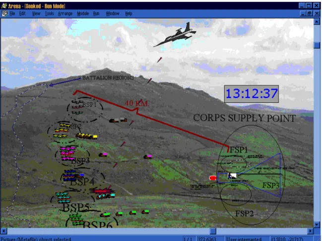
• The errors in the model can also be observed through animation. Animation presents a dynamic moving picture of the entities within the simulation. Thus, it is very powerful tool in model verifications. Arena enables us to create an animation of the model. During model development, the animation of our model helped us to find the errors and correct them. A sight from this animation is given in Figure 3.4.
3.4.2. Validation
Validation is concerned with building the right model. It is utilized to determine that a model is an accurate representation of the real system. It is the overall process of comparing the model and its behavior to the real system and its behavior. We followed the following steps in the validation process.
3.4.2.1. Face Validity
Face validity is achieved by asking people familiar and knowledgeable about the real system whether the model and/or its behavior appear reasonable. Potential users of a model should also be involved in model construction from its conceptualization to its implementation to ensure that a high degree of realism is built into the model (Banks 1999). From the beginning of our study, we include the users in the process of model development. Thus we assure that the model behaves as expected. The outputs of the simulation model is also found to be quite reasonable by the officers in the Logistics Information Systems Center. The output of one replication from our simulation model is given in Appendix H.
3.4.2.2. Sensitivity Analysis
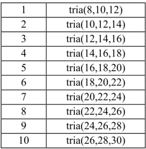
Sensitivity Analysis can be used to check the validity of the model. For example, in real-world system, an increase on the loading times in corps supply point must cause the maximum time-in-system performance measure to increase. As seen in Figure 3.5, our simulation model behaves as we expect in real-world system. The x-axis of the graph shows the points of experiment (Table 3.5).
Figure 3.5. Sensitivity Analysis on the Loading Times
Table 3.5. Points of Experiment for The Sensitivity Analysis on Loading Times 1 tria(8,10,12) 2 tria(10,12,14) 3 tria(12,14,16) 4 tria(14,16,18) 5 tria(16,18,20) 6 tria(18,20,22) 7 tria(20,22,24) 8 tria(22,24,26) 9 tria(24,26,28) 10 tria(26,28,30)
Both face validity and sensitivity analysis indicate that our model is an accurate representation of the real supply system, and it behaves as expected.
0 100 200 300 400 500 600 0 1 2 3 4 5 6 7 8 9 10 Points of Experiment
Maximum Time in System
Chapter 4
Design and Analysis of the Experiments
Experiments are performed by investigators in virtually all fields of inquiry, usually to discover something about a particular process or system. Literally, an experiment is a test. A designed experiment is a test or series of tests in which purposeful changes are made to the input variables of a process or system so that we may observe and identify the reasons for the changes in the output response (Montgomery 1991).
In this part of our study, we look for the answers of following research questions: • Does any bottleneck occur in the system ?
• How do artillery and air attacks of enemy affect the system performances ? • What happens if we change the organization of the facilities in the food supply
system ?
• What are the significant factors and how do they affect the system performance measures ?
4.1. 2
5Factorial Designs
If we wish to draw meaningful conclusions from an experimental design, we have to implement statistical methods. These methods require that observations should be independently distributed random variables. This is achieved in simulation experiments by taking independent replications. Another important point in experimental designs is the selection of an appropriate sample size. We apply the Sequential Procedure proposed by Law and Kelton (1991) to achieve a certain accuracy. Pilot experiments indicate that 15 replications are enough to estimate MTIS and
number-of-destroyed-vehicles performance measures with %95 accuracy. Details of the calculations, and the application of Sequential Procedure are given in Appendix C.
Our experiment involves the study of the main and interaction effects of 5 factors on the following performance measures.
• Maximum time in system • Number of destroyed vehicles
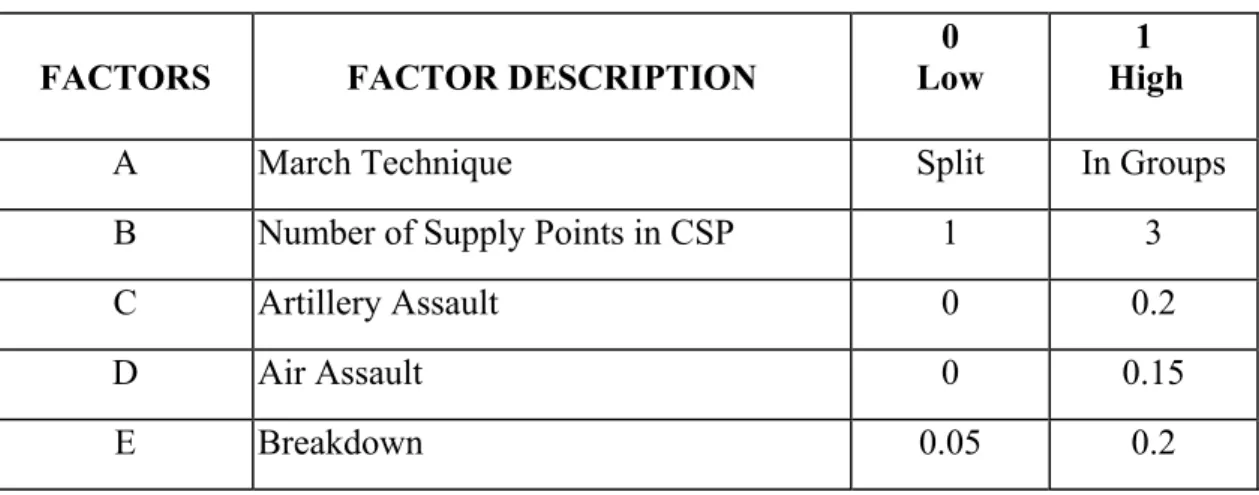
We implement 2k factorial design to identify the significant factors and their interactions. We have 5 factors. Factor A is the march technique on which Convoy Commander of the vehicles decides. During traveling, especially under enemy attack, some of the vehicles will have breakdown and should be repaired immediately. In this technique, we consider two cases: split&group. In the split case, the vehicles which don’t have breakdown do not wait for the breakdown vehicles to be repaired and go on their march. However, in the group case, convoys move in group. At times of breakdown of some vehicles, the rest of convoy wait for the failed vehicles to be repaired. Hence, in the group case, the convoy cannot split and goes on its movement in integrity. Factor B is the number of food supply points in Corps Supply Point. The number of these facilities can be at least 1 and at most 3. Factor C, D, E are enemy artillery attack, enemy air attack and the usual breakdowns, respectively. Since the food supply system operates in the rear region of Army Corps, the air and artillery attacks of enemy are not highly expected. Therefore, we define the low levels of factor C and factor D as having 0 probability and define the high levels as having 0.2 and 0.15 probabilities, respectively. The officers in Logistics Information Systems Center helped us during the determination process of the levels of these factors. In Table 4.1, factor
descriptions and the levels of the factors are presented. Note that factor A and factor B are controllable and the factors C, D, E are uncontrollable factors.
Table 4.1. Description and Levels of Factors
FACTORS FACTOR DESCRIPTION Low 0 1 High
A March Technique Split In Groups
B Number of Supply Points in CSP 1 3
C Artillery Assault 0 0.2
D Air Assault 0 0.15
E Breakdown 0.05 0.2
4.2. Diagnostic Checking on The Validity of Assumptions
Recall that, we have 25 design points. Each of these design points is called as a treatment. After we have made 15 replications for each treatment, we perform ANOVA to identify significant factors and their interactions. The outputs of 32 treatments are given in Appendix D.Before the evaluation of these ANOVA results for each performance measure, we should check the validity of two important assumptions of ANOVA. The first one is the normality of the errors and the second one is homogeneity of variances across the treatments. Violations of these assumptions can be examined by the examination of the residuals.
The residuals for our model can be defined as; ei= yi. - ŷi i=1,2,...32 ; j=1,2,...15
where i is the treatment number
yi. is the observed mean of the ith treatment
ŷi is the predicted value of mean for the ith treatment
We computed ŷi ’s via a regression model which is given in Appendix E. The
residuals for each performance measure are tested to see whether they fit a normal distribution or not. We found that the residuals are normally distributed according to Kolmogorov-Smirnov and Anderson-Darling tests. The summary of these test results are given in Table 4.2.
Table 4.2. The Results of Kolmogorov-Smirnov and Anderson-Darling Tests Test Statistic Critical Value P value Result
MTIS K – S 0.188 0.234 0.182 Do not reject H0
A – D 1.730 2.490 0.130 Do not reject H0
DEST K – S 0.206 0.234 0.114 Do not reject H0
A – D 1.060 2.490 0.329 Do not reject H0
where K-S and A-D tests the following hypotheses ; Ho : The residuals fit the normal distribution
H1 : Above is not true
MTIS stands for the Maximum Time-In-System performance measure and DEST stands for the number of destroyed vehicles. In Appendix F, we present the residuals calculated via the regression models.
In order to check the homogeneity of variances across the treatments for the maximum time in system performance measure, we applied the Bartlett test. We simply tested the following hypothesis.
Ho : σ12 =σ22 =...=σ322
H1: above is not true for at least one σi2
The test statistic is χ02 = 2.3026(q / c) where
The quantity q is large when the sample variances Si2 differ greatly and is equal to
zero when all Si2 are equal. Therefore, we should reject Ho on values of χ02 that are too
large; that is, we reject Ho only when χ02 > χα,a-12.
The results indicate that we reject the null hypothesis for the maximum timein -system performance measure (Table 4.3). It means that the variances across the treatments are not homogeneous. The usual approach to deal with this problem is to apply a variance-stabilizing transformation (Montgomery 1991).
Table 4.3. Result Of Bartlett Test for MTIS Performance
Measure Sp2 Q C
χ
02χ
α,a-12 ResultMTIS 15.516 83.504 1.024 187.679 44.97 Reject H0 2 2 10 10 1 ( ) log p a ( i 1) log i i q N a S n S = = − −
∑
− 1 1 1 1 1 ( ( 1) ( ) ) 3( 1) a i i c n N a a − − = = + − − − −∑
2 2 1 ( 1) a i i i p n S S N a = − = −∑
Before transformation, we empirically examine the variances of the treatments and find that the variance of treatments in which factor A is at its low level and the variance of treatments in which factor A is at its high level differs significantly. We have the same observation for factor D. Then we first omit factor A and made 24 factorial design and test the variances of treatments again but the variances are found to be not homogenous. Then factor D is omitted and the same procedure above is followed but we found that the variances across the treatments are still not homogenous. At this point we decided to apply a variance-stabilizing transformation.
If the theoretical distribution of the observations is known, this knowledge can be utilized in selecting the transformation. But in our case we don’t have any information. Thus, we empirically seek a transformation that equalizes the variances across the treatments (Montgomery 1991). After we applied the logarithmic transformation, we observed that these transformed data pass the Bartlett test (Table 4.4). We can feel confident about the transformation because it stabilizes the variances across the treatments and the ANOVA results for actual data and the transformed data are mostly parallel to each other. The ANOVA of performance measures was performed in SPSS software and presented in Appendix G.
Table 4.4. Result of Bartlett Test for MTIS (Transformed Data) Performance
Measure Sp2 Q C
χ
02χ
α,a-12 ResultMTIS 1.84E-05 -14.379 1.024 -32.316 44.97 Do not Reject H0
We can not apply the Bartlett Test to check the homogeneity of variances for the number of destroyed vehicles performance measure. Because we have some treatments in which variance is zero. Therefore we analyzed the scatter plots of residuals and variances (Figure 4.1 and Figure 4.2). Since these plots are structureless and do not contain an obvious pattern, we can conclude that the variances across the treatments for the number of destroyed vehicles performance measure are homogeneous.
Figure 4.1. Scatter Plot of Variances for Number Of Destroyed Vehicles
Figure 4.2. Scatter Plot of Residuals for Number of Destroyed Vehicles
Scatter Plot of Residuals for The
Number of Destroyed Vehicles
-1,0 -0,5 0,0 0,5 1,0 1,5 0 10 20 30 40 Residuals
Scatter Plot of Variances for The
Number of Destroyed Vehicles
0 0,2 0,4 0,6 0,8 1 1,2 1,4 0 5 10 15 20 25 30 35 Variances
4.3. Evaluation of Main and Interaction Effects of Maximum
Time in System
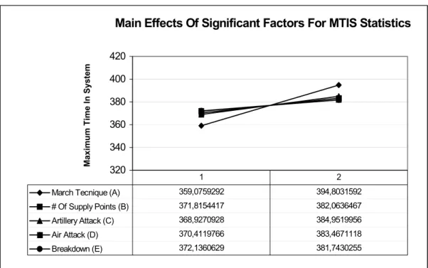
The results of ANOVA which is performed in SPSS software indicate that march technique, number of food supply points in Corps Supply Point, enemy attacks and the usual breakdown are significant factors. We also found that the interactions between march technique and number of FSPs, march technique and enemy air attack, and march technique and breakdown are all significant. We further examine these significant main and interaction effects by plotting diagrams. We show the main effects of significant factors in Figure 4.3.
Figure 4.3. Main Effects of Significant Factors for MTIS
Main Effects Of Significant Factors For MTIS Statistics
320 340 360 380 400 420 Maxi mu m T ime I n System
March Tecnique (A) 359,0759292 394,8031592
# Of Supply Points (B) 371,8154417 382,0636467
Artillery Attack (C) 368,9270928 384,9519956
Air Attack (D) 370,4119766 383,4671118
Breakdown (E) 372,1360629 381,7430255
The line of march technique has steeper increase than the lines of other factors. It means that the main effect of this factor is greater than the effects of other factors. As discussed earlier, the low level of march technique is the split form. If a convoy can split at times of breakdown, the majority of the convoy do not wait for the failed vehicles to be repaired. Hence, this will cause the maximum time-in-system to decrease.
Enemy attacks and usual breakdown are significant. Because the number of damaged vehicles which are to be repaired at the high levels of these factors are more than the number at the low level of these factors. Thus, repairing the damaged vehicles when these factors are at their high levels takes much time and there will be an increase on maximum time in system.
When the number of food supply points (Factor B) is three, one of the FSPs operates as the main point and serves only for the third and fourth brigade convoys. The first, the second, the fifth and the sixth brigade convoys are served by the remaining two FSPs. These remaining two FSPs do not have the all needed food in their depots. Therefore, some of the vehicles of 1st , 2nd , 5th , 6th brigade convoys have to be served from main FSP. But these vehicles have to wait for the 3th and 4th brigade convoys to be loaded first. If the number of FSPs is one, none of the convoys has priority over the other convoys. Because there are six loading teams inside this FSP and each of these teams will only serve one brigade convoy. We can conclude that when factor B is at its high level, some of the vehicles from 1st , 2nd , 5th , 6th brigade convoys have to move toward the main FSP and have to wait for the 3th and 4th brigade convoys to be loaded. Hence, these activities will cause maximum time in system to increase.
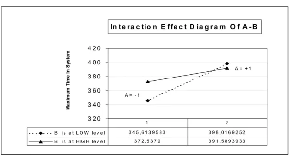
The interactions between the factor is investigated in our study. The interaction between march technique and number of supply points is presented in Figure 4.4. The
permanent line shows the change in maximum time-in-system measure while factor B is at lowest level and factor A is shifting from 0 (split) to 1 (group). The dotted line shows the change in maximum time in system measure while factor B is at highest level and factor A is shifting from 0 (split) to 1 (group).
Figure 4.4. The Interaction Effect Between Factor A and Factor B for MTIS
Because of the interaction between factor A and factor B, the interpretation of main effects of factor A and factor B may be a little subjective. Because a significant interaction will mask the significance of main effects. In our study, the average of MTIS across the treatments when factor A is at its low level is 359.07. But when both factor A and factor B is at low levels, the average of MTIS decreases to 345.61 and when factor A is at low level again and factor B is high level, the average of MTIS increases to 372.53 at this time.
It means that while convoys march in split form, they do not wait so much in the loading queues when there is one FSP (low level of factor B) as they wait in the loading
In te r a c tio n E ffe c t D ia g r a m O f A -B A = + 1 A = - 1 3 2 0 3 4 0 3 6 0 3 8 0 4 0 0 4 2 0 M axim u m Tim e In System B is a t L O W le v e l 3 4 5 ,6 1 3 9 5 8 3 3 9 8 ,0 1 6 9 2 5 2 B is a t H IG H le v e l 3 7 2 ,5 3 7 9 3 9 1 ,5 8 9 3 9 3 3 1 2
queues when there are three FSPs. The case is different when factor A is at high level. Because the average of MTIS is 394.80 at the high level of factor A whereas the average is 391.58 when factor A and factor B are at high levels and it is 398.01 when factor A is again high level and factor B is low level. Actually there is not so much difference between these values. Since the convoys march in groups and arrive FSPs in that form, the average waiting time in the loading queues do not change so much whether the number of FSPs is one or three. To shift the march technique from high level (in groups) to low level (split) will cause the average waiting time in the loading queues at FSPs to decrease and this change will decrease the MTIS either as seen in Figure 4.4.
In Figure 4.5, we plot the interaction effect of factor A and factor C. The dotted line shows the change in MTIS measure when factor C (enemy artillery attack) is at high level and factor A is shifting from low to high level. On the other hand, the permanent line shows the change in MTIS measure when factor C is at low level and factor A is shifting from low to high level.
Figure 4.5. The Interaction Effect Between Factor A and Factor C for MTIS
In te r a c tio n E ffe c t D ia g r a m o f A -C A = - 1 A = + 1 3 2 0 3 4 0 3 6 0 3 8 0 4 0 0 4 2 0 Maxi mum Ti me I n S ystem C is a t L O W le v e l 3 5 4 ,0 3 5 1 9 9 3 3 8 3 ,8 1 8 9 8 6 3 C is a t H IG H le v e l 3 6 4 ,1 1 6 6 5 9 4 0 5 ,7 8 7 3 3 2 1 1 2
When the artillery forces of enemy launches an attack on convoys, the number of damaged and destroyed vehicles increases. Thus, repairing them will take much time. The average waiting time in repair queue while the convoys march in groups during this artillery attack is slightly much than the one while they move in split form. That is why the dotted line is a bit steeper than the permanent line.
The diagram of interaction effect between march technique and usual breakdown is presented in Figure 4.6.
Figure 4.6. The Interaction Effect Between Factor A and Factor E for MTIS
In our model, the drivers are authorized to repair their vehicles if first type of usual breakdown occurs. As seen in Figure 4.6, MTIS does not change so much when factor A is at low level (split) while the probability of breakdown shifts from 0.05 to 0.2. Because the average number of vehicles which had first type breakdown is less than the average number of vehicles which have second type breakdown when factor A is at low level. But when factor A is at high level the average number of vehicles which had
I n te r a c ti o n E ffe c t D i a g r a m o f A -E A = - 1 A = + 1 3 2 0 3 4 0 3 6 0 3 8 0 4 0 0 4 2 0 M a x imum Time In Sy s te m E is a t L O W le v e l 3 5 9 ,4 3 9 9 0 4 9 3 8 4 ,8 3 2 2 2 0 9 E is a t H IG H le v e l 3 5 8 ,7 1 1 9 5 3 4 4 0 4 ,7 7 4 0 9 7 5 1 2
second type of breakdown is slightly more than the average number of vehicles which have first type of breakdown. Since the second type of usual breakdown can only be repaired by technician and his team, the average number of vehicles waiting in repair queue increases and this cause MTIS to increase slightly either.
4.4. Evaluation of Main And Interaction Effects for The
Number of Destroyed Vehicles Statistics
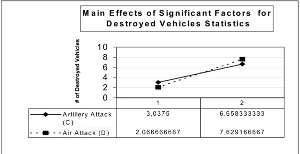
The results of ANOVA for this performance measure indicate that artillery and air attacks of enemy are significant factors. There is a slight interaction effect between these factors too. The main effects of these significant factors are presented in Figure 4.7.
Figure 4.7. Main Effects of Significant Factors for Number of Dest. Vehicles
M a in E ffe c ts o f S ig n ific a n t F a c to r s fo r D e s tr o y e d V e h ic le s S ta tis tic s 0 2 4 6 8 1 0 # o f Dest ro yed Veh icl es A rtillery A ttac k (C ) 3 ,0 3 7 5 6 ,6 5 8 3 3 3 3 3 3 A ir A ttac k (D ) 2 ,0 6 6 6 6 6 6 6 7 7 ,6 2 9 1 6 6 6 6 7 1 2
The permanent and the dotted lines show the change in the number of destroyed vehicles while the underlying factors shift from low level to high level. The dotted line is a little steeper than the permanent line. Since the kill probability in air attacks is higher than the one in artillery attacks the average number of destroyed vehicles due to air attack will be more than the average number of vehicles which is destroyed by enemy artillery attack.
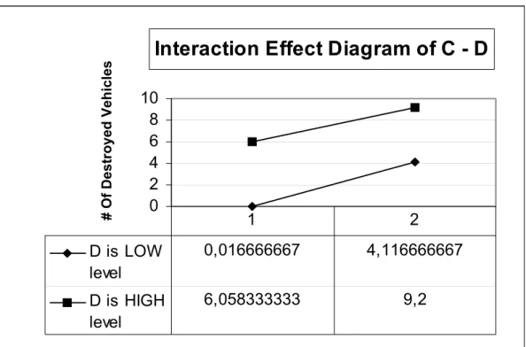
In Figure 4.8, we plot the interaction effect between artillery and air attacks of enemy. The inference drawn from this diagram is that the lines are almost parallel to each other. Hence, we can say that the interaction effect between these factors are negligible.
Figure 4.8. The Interaction Effect Diagram of Factor C and Factor D
Interaction Effect Diagram of C - D
0 2 4 6 8 10 # Of Destroyed Vehicles D is LOW level 0,016666667 4,116666667 D is HIGH level 6,058333333 9,2 1 2
4.5. Sensitivity Analysis
In this section, we investigate whether maximum time-in-system performance measure is sensitive to the changes in the variances of loading distributions. As seen in Table 4.6, MTIS and average time-in-system measures do not follow a decreasing or increasing pattern. It means that if the loading activities are performed with equipments such as forklifts, the variability in the loading times will decrease but this decrease does not cause a decrease on maximum time-in-system measure in our system. If we somehow decrease the mean times during loading, we achieve a decrease on MTIS measure (Table 4.7)
Table 4.6. Sensitivity Analysis (I)
Points of Experiment Mean Variance MaxTIS AvTIS
tria(8.0,10,12.0) 10 0.6666 378.08 321.64 tria(8.2,10,11.8) 10 0.5400 384.92 324.78 tria(8.4,10,11.6) 10 0.4266 385.25 323.50 tria(8.6,10,11.4) 10 0.3266 385.11 323.56 tria(8.8,10,11.2) 10 0.2400 377.83 321.54 tria(9.0,10,11.0) 10 0.1666 390.85 325.54 tria(9.2,10,10.8) 10 0.1066 394.88 329.90 tria(9.4,10,10.6) 10 0.0600 391.98 330.56 tria(9.6,10,10.4) 10 0.0260 380.50 322.04 tria(9.8,10,10.2) 10 0.0066 381.31 322.16 tria(10,10,10) 10 0.0000 378.61 322.37
Table 4.7. Sensitivity Analysis (II)
Points of Experiment Mean Variance MTIS ATIS
tria(8,10,12) 10 0.6666 378.08 321.64 tria(7,9,11) 9 0.6666 383.06 315.34 tria(6,8,10) 8 0.6666 363.74 308.56 tria(5,7,9) 7 0.6666 351.15 299.45 tria(4,6,8) 6 0.6666 351.87 293.45 tria(3,5,7) 5 0.6666 342.63 285.22 tria(2,4,6) 4 0.6666 338.28 284.08 tria(1,3,5) 3 0.6666 337.30 275.80
4.6. Conclusion
For MTIS performance measure, the main effects of all factors are significant. March technique is the most significant factor. There are also three significant interactions for MTIS: March technique-number of FSPs, march technique-artillery assault, and march technique-breakdown.
Time is one of the most important criteria in making logistic plans. The information obtained from Chapter 4 indicates that staff officers who are assigned to prepare these plans should carefully examine the effects of enemy attacks, breakdowns, and especially the choice of march technique. If the technology which makes the control, coordination, and command activities of convoys easy exists, planners should prefer the split form during the decision process for the appropriate march technique. As stated before, occurrence of enemy attacks means there will be failed vehicles to be repaired. Hence, this will cause time measure to increase. If security precautions of convoys during traveling are enhanced, the damage taken by these enemy attacks will be less. Breakdown causes time measure to increase significantly. Therefore, the maintenance of vehicles in peace time carries a great importance.
For the number-of-destroyed-vehicles performance measure, artillery and air assaults are significant factors. The interaction between these factors are slightly significant. The results indicate that enemy attacks may handicap the supply system. In order to prevent the enemy attacks, commanders must give more importance to reconnaissance activities to anticipate these attacks.
Since supply points are well protected against the artillery and air attacks of enemy, we assumed that the convoys are safe when they arrive FSPs. Hence, it is usual
to observe that number of FSPs is an insignificant factor for the number-of-destroyed-vehicles performance measure. Selection of march technique doesn’t affect the occurrence of enemy attacks. Hence, it is again usual to observe that this factor is insignificant for the number-of-destroyed-vehicles performance measure. During model development, we assumed that engines of the vehicles are in good condition. The results obtained from experiments indicate that the average number of destroyed vehicles across all treatments as a result of breakdown are mostly zero. That is why breakdown factor is insignificant for the number-of-destroyed-vehicles performance measure. Since artillery and air attacks are two independent activities of enemy, it is usual to observe insignificant interaction between these factors for MTIS performance measure. We summarize the significant factors and interactions for each performance measure in Table 4.5.
Table 4.5. Significant Factors and Interactions for Performance Measures
Factors and Interactions MTIS DEST.
March Technique Significant Insignificant
Number of FSPs Significant Insignificant
Artillery Assault Significant Significant
Air Assault Significant Significant
Breakdown Significant Insignificant
March Technique - Number of FSPs Significant Insignificant March Technique - Artillery Assault Significant Insignificant March Technique – Breakdown Significant Insignificant Artillery Assault - Air Assault Insignificant Significant
Chapter 5
Implementation of Analytic Hierarchy Process for Army
Corps Food Supply System
5.1. Introduction
In the previous chapter, we found out that factor A, factor B, and their interactions are significant for MTIS performance measure. To decide on the number of FSPs and the march technique is an important decision for staff officers who prepare logistic plans. At this point, we make three alternatives from these configurations of the factors (Table 5.1) to help the officers in their decision process. In the first alternative, there is only one FSP and convoys move in split form. The second alternative is that there are three FSPs and the convoys move in split form. In the third one, there is one FSP and convoys move in group. Note that there are three FSPs and convoys march in group in the existing system. We call the existing system as the fourth alternative for the simplicity in further explanations.
Table 5.1. Alternative Designs for The Army Corps Food Supply System
Alternative Number of FSP March Technique
1 1 Split
2 3 Split
3 1 Group
4 3 Group
In terms of MTIS, Alternative-1 is 349.21 which is best when it is compared with other alternatives. The results given in Table 5.2 are found quite reasonable by the