Abstract— A noiseless image is desirable for many applications. However, this is not possible. Generally, wavelet-based methods are used to noise reduction. However, due to insufficient performance of wavelet transforms (WT) on images, different multi-resolution analysis methods have been proposed. In this study, one of them is Contourlet Transform (CT) and the Translation-Invariant Contourlet Transform (TICT) which is an improved version of CT is compared using different noises. The fundus images are taken from the DRIVE dataset and benchmark images are used. Peak Signal-to-Noise Ratio (PSNR), Mean Squared Error (MSE), Mean Structural Similarity (MSSIM) and Feature Similarity Index (FSIM) are used as comparison criteria. The results showed that TICT is better in Gaussian noisy images.
Index Terms—Contourlet Transform, Image Denoising, Time
Invariant Contourlet Transform
I. INTRODUCTION
N RECENT years, many algorithms have been developed for image processing [1-3]. Therefore, digital image processing has been available in some areas, such as physics, defense industry, medicine, industrial applications, robotics, intelligent transportation systems, etc [4]. Considering the application fields, it is understood that it is used for important and sensitive tasks. However, in the process of obtaining an image, noise occurs on the image. This may be caused by the quality of the camera or the environment conditions. According to Patil [5], there is no noiseless signal.
MUHAMMET FATIH ASLAN, is with Department of Electrical and Electronic Engineering, Karamanoglu Mehmetbey University, Karaman, Turkey,(e-mail: [email protected]).
https://orcid.org/0000-0001-7549-0137
KADIR SABANCI, is with Department of Electrical and Electronic Engineering,Karamanoglu Mehmetbey University, Karaman, Turkey, (e-mail:
https://orcid.org/0000-0003-0238-9606
AKIF DURDU, is with Department of Electrical and Electronic Engineering, Konya Technical University, Konya, Turkey, (e-mail: [email protected]).
https://orcid.org/0000-0002-5611-2322
Manuscript received June 03, 2019; accepted September 16, 2019. DOI: 10.17694/bajece.573583
An image can also be considered as a 2D signal. Therefore, no image or video obtained can be noiseless. Therefore, it is necessary to remove the noise in order to obtain results that are more accurate.
There are many kinds of noise that can cause the image distortion. In general, noise types are Gaussian noise, Random noise, Salt and Pepper noise, Poisson noise, and Speckle noise [6]. Particularly in the case of remote sensing applications, the majority of the problem is caused by Speckle noise. Speckle noise directly reduces the quality of the image [7].
Denoising or noise reduction includes applications for removing noise that occurs after the image has been acquired. Different statistical methods have been developed to image enhancement [8, 9]. However, these methods blur the edges with a low pass filter for spatial filtering problems. It also strengthens the background with high-pass filter [10]. Linear techniques are also used in denoising. However, in the case of impulsive noise, such filters are insufficient [6]. Fourier Transform (FT) is also an alternative for denoising. But, while FT provides frequency resolution, it does not provide a time resolution. Therefore, the spatial location of the frequency change due to noise at one point cannot be determined. This problem can be solved by Short Time Fourier Transform (STFT), but in STFT method the window width is constant. A large window provides good frequency resolution but causes poor time resolution. Likewise, a narrow window provides good time resolution, but the frequency resolution is poor [11]. Therefore, the window width should not be constant and the window width should be changed depending on the frequency. This situation can be achieved by the wavelet transform which also includes the scale variable.
Wavelet transform (WT) is a time-scale analysis method used in image compression [12], edge detection [13] and deconvolution [14], besides image denoising [6]. There is an inverse relationship between the scale and the frequency. Wavelet algorithms process data at different scales or resolutions. By comparing the signal and wavelet in different scales and positions, a two-variable function is obtained. A smaller scale factor means more compression of the wavelet. Thanks to scaling, high frequency behaviors at low scales and low frequency behaviors at high scales are better analyzed. This is very important for non-stationary signals.
Comparison of Contourlet and Time-Invariant
Contourlet Transform Performance for Different
Types of Noises and Images
M. F. ASLAN, K. SABANCI and A. DURDU
The WT of a continuous signal is called the Continuous Wavelet Transform (CWT). Due to the CWT requires an infinite number of inputs, it is not suitable for the computer. It also has a disadvantage in terms of speed. Therefore, the Discrete Wavelet Transform (DWT) is used for computer-based systems. While the scale (s) and position (𝜏) parameters are real numbers in the CWT, they get an integer value in DWT. DWT occurs by sampling the CWT.
The signal consisting of a discrete time series in DWT is divided into different frequency ranges. Because of this, the original signal is passed through the high-pass filters (HPF) and the low-pass filters (LPF), and the image or signal is divided into subbands. Then, time series are divided into low frequency (Approximation (A)) and high frequency (Detail (D)) components. As a result, approximate and detail coefficients are obtained. The coefficient A represents the low-frequency values in the time series, and the D coefficient represents the high-frequency values of the time series. This process may continue iteratively. Thus, the multi-resolution analysis (MRA) of the signal/image in the frequency domain is obtained [15, 16].
Wavelet-based transforms analyze the signal in the frequency-time domain. This corresponds to edge detection in the images. Edge information is a feature that best describes an image. One-dimensional transforms such as Fourier and WT are commonly used in capturing edges. In an image, one-dimensional edges, such as scan lines, are well decomposed by wavelets. However, the edges in natural images are not limited to this. The points of discontinuity can lie along the curve depending on an object in the image. Most of the natural images contain intrinsic geometric structure. Due to the WT is a one-dimensional transform, images are applied to the row and column for WT. For 2D data, the wavelets are well decomposed to the discontinuities at the edge points, but cannot smooth and continuously represent the edge points along the curve. In addition, WT has limited directional information [17]. WT is not given good results in speckle noise reduction [18]. Different MRA methods have been developed to solve such problems. For example, in the Ridgelet transform [19], angular windows are used, so that unlike WT, data is processed in different directions. In curvelet transform [20], windows are applied along second order curves. For Ripplet transform [21], the window is applied along the higher order curve. In the Tetrolet transform [22], the image is divided into 4x4 blocks. The most appropriate tetromin is selected for each block and applied WT to this region [23]. The Contourlet Transform (CT) [17] used in this study analyzes the smoothness along the contours better than WT by using the multiresolution and direction filter.
Denoising has always been one of the main problems in image processing. It is always desirable to protect edges, corners and other important features during the image denoising process. Image denoising is a highly needed method, especially in biomedical applications. Saha, et al. [24] introduced two mathematical transforms, wavelet and curvelet, in the field of biomedical imaging. Applications of the two transforms were compared using biomedical images. Jain and Tyagi [25]
proposed a new edge preserving image denosising method based on adaptive thresholding method and Tetrolet transform. The noisy image is decomposed into the tetrolet coefficients via a tetrolet transform. Using the locally adaptive threshold, the tetrolet coefficients are thresholded to effectively reduce noise while preserving the necessary features of the image. Huang, et al. [26] presented a novel multiscale approximation method called adaptive digital ridgelet (ADR) transform. Unlike conventional transform methods, this algorithm can adaptively handle line and curve information in an image, taking into account its infrastructure. Using a new curve part detection method, the curve parts in an image are detected. When this method was applied experimentally, successful results were obtained in image denoising application.
In this study, image denoising was performed. The CT and the TICT methods developed by Eslami and Radha [27]were used. The denoising application was made using the fundus and benchmark images. The performance of both methods was compared by using different noise and different noise ratios. In [27], TICT and STICT have been proposed as an alternative to CT and comparisons have been made. However, comparisons were made using Gaussian white noise. Noise types vary depending on the image used and the application field. Therefore, it would be appropriate to determine the transform method according to the noise distribution. For example, the noise distribution in traditional magnitude MR images is Rician [28]. Therefore, the aim of this article is to observe the results of TICT and CT at different noise distributions.
II. CONTOURLET TRANSFORM
Fourier and WT are 1D transform developed to capture discontinuous points. Therefore, the contours of the internal geometric shapes found in an image are determined locally by these transforms. Thus, the geometric smoothness of the contours cannot be achieved. To achieve smoothness along the contour in multi-dimensional signals, CT has been developed. Do and Vetterli [17] indicated the difference between WT and CT with Fig. 1. While only point discontinuities can be captured with wavelets according to Fig. 1, the series of linear points can be captured with CT. Thus, the image is represented with less coefficient.
(a) WT (b) CT Fig. 1. Edge catching strategies using WT and CT
The double filter structure is used in CT. Firstly, Laplacian pyramid (LP) [29] is used to capture discontinuities in the image. The discontinuous points have been achieved as a result
of this. After that, the Directional Filter Bank (DFB) [30] is applied to transform discontinuous points into smooth geometric shape contours (see Fig. 2). In fact, the contour components obtained by decomposition are combined with the DFB. Combined contours can be in different direction and scale. In this way, more continuous edge points are achieved than WT. This can be easily understood from Fig. 3.
Fig. 2. The structure of CT [31]
(a) WT (b) CT Fig. 3. Transforms for the same image [17]
III. TRANSLATION-INVARIANT CONTOURLET TRANSFORM The energy calculated by the analysis of a wave using DWT is different from the energy calculated by the shift of the same wave. This is called a time-variant. Since LP and DFB resemble WT in terms of sub-sampling, CT is time-variant. To improve performance in image denoising, transform should be translation-invariant (time-invariant). Therefore, Translation-Invariant Contourlet Transform (TICT) by Eslami and Radha [27] was proposed. The big benefit of time invariant is that the performance of denoising studies is significantly improved when a time invariant scheme of subsampled transform is used [27]. Since the CT sub-sampled LP and DFB included, the TI method was applied at both process to generate a TICT.
IV. APPLICATION AND RESULTS
In this study, five benchmark images and 40 fundus images taken from the DRIVE dataset [32] were used (see Fig. 4.). The used benchmark images and some fundus images are shown in Fig. 4. Firstly, Random, Gaussian and Rician noises were added to these images respectively (sigma = 5, 10, 15 for Random noise; signal-to-ratio (snr) = 3, 5, 10 for Gaussian and Rician noise). Equations of these noise distributions are shown below respectively. 𝐷1 = 𝐼 + 𝑠𝑖𝑔𝑚𝑎 𝑥 𝑟𝑎𝑛𝑑(𝑠𝑖𝑧𝑒(𝐼)) (1) 𝐷2 = 1 𝜎√2𝜋𝑒 −(𝑥−𝑢)2 2𝜎2 (2) 𝐷3 =𝑀 𝜎2𝑒 𝑀2+𝐴2 2𝜎2 𝐼 0( 𝐴 𝑥 𝑀 𝜎2 ) (3)
In Equation 1 above, I represents the source image. In Equation 2, X is a random variable. It is usually shown as follows.
𝑋~𝑁((𝜇, 𝜎2) (4)
In Equation 4, μ is the mean value of the Gaussian distribution. σ is the standard deviation value.. In Equation 3, 𝐼0 is the modified zeroth-order of Bessel function of the first kind. This is called as Rice density. M is observed noisy intensity and A is true signal intensity [33].
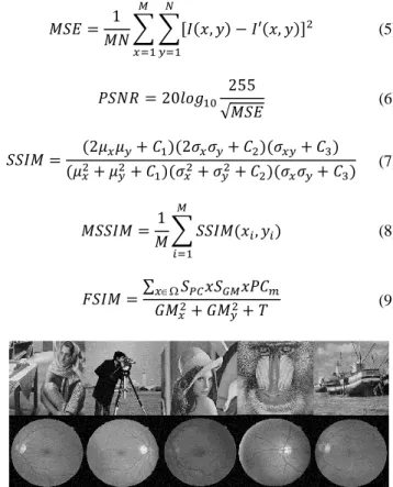
After the noise is added, these distorted images were analyzed using CT and TICT. The threshold were applied to the components obtained and then reconstruction was performed. As a result, the result image was compared to the original image. MSE, PSNR, MSSIM and FSIM metrics were used as comparison criteria. The mathematical expression of these metrics is shown below. 𝐼(𝑥, 𝑦) in Equation 5 represents the source image. 𝑀 and 𝑁 are image sizes. 𝐶1, 𝐶2, 𝐶3 in Equation 7 are constant values. 𝜇 and 𝜎 are mean values and standard deviation, respectively. The FSIM in Equation 9 is a metric based on phase congruency (𝑃𝐶) and gradient magnitude (𝐺𝑀). 𝑆𝑃𝐶 is a local similar map of 𝑃𝐶 between 𝑃𝐶𝑥 and 𝑃𝐶𝑦. 𝑆𝐺𝑀 is a local similar map of 𝑃𝐶 between 𝐺𝑀𝑥 and 𝐺𝑀𝑦. 𝑇 is a constant value [34]. The results obtained using the metrics described below are shown in Table I and Table II.
𝑀𝑆𝐸 = 1 𝑀𝑁∑ ∑[𝐼(𝑥, 𝑦) − 𝐼′(𝑥, 𝑦)] 2 𝑁 𝑦=1 𝑀 𝑥=1 (5) 𝑃𝑆𝑁𝑅 = 20𝑙𝑜𝑔10 255 √𝑀𝑆𝐸 (6) 𝑆𝑆𝐼𝑀 = (2𝜇𝑥𝜇𝑦+ 𝐶1)(2𝜎𝑥𝜎𝑦+ 𝐶2)(𝜎𝑥𝑦+ 𝐶3) (𝜇𝑥2+ 𝜇𝑦2+ 𝐶1)(𝜎𝑥2+ 𝜎𝑦2+ 𝐶2)(𝜎𝑥𝜎𝑦+ 𝐶3) (7) 𝑀𝑆𝑆𝐼𝑀 = 1 𝑀∑ 𝑆𝑆𝐼𝑀(𝑥𝑖, 𝑦𝑖) 𝑀 𝑖=1 (8) 𝐹𝑆𝐼𝑀 =∑𝑥𝑆𝑃𝐶𝑥𝑆𝐺𝑀𝑥𝑃𝐶𝑚 𝐺𝑀𝑥2+ 𝐺𝑀 𝑦2+ 𝑇 (9)
TABLE I
DENOISING PERFORMANCE RESULTS OF FUNDUS IMAGES
Type of Noise Noise Ratio Evaluation Criteria CT TICT
Random Sigma=5 PSNR 40.1699 40.1634 MSE 6.2531 6.2624 MSSIM 0.1773 0.0605 FSIM 0.8268 0.9143 Sigma=10 PSNR 34.1521 34.1429 MSE 24.9962 25.0492 MSSIM 0.0914 0.0132 FSIM 0.8061 0.9014 Sigma=15 PSNR 30.6288 30.6219 MSE 56.2608 56.3497 MSSIM 0.0573 0.0048 FSIM 0.7963 0.8964 Gaussian Snr=3 PSNR 23.5333 27.4376 MSE 301.4683 120.1661 MSSIM 0.7279 0.6507 FSIM 0.8684 0.9735 Snr=5 PSNR 23.9313 29.4056 MSE 275.8284 76.3219 MSSIM 0.7513 0.7233 FSIM 0.8694 0.9769 Snr=10 PSNR 24.3999 34.0896 MSE 248.3114 25.7974 MSSIM 0.7969 0.8520 FSIM 0.8696 0.9819 Rician Snr=3 PSNR 37.4514 37.4403 MSE 11.6957 11.7256 MSSIM 0.1514 0.0235 FSIM 0.7878 0.9044 Snr=5 PSNR 32.6911 32.6777 MSE 34.9946 35.1029 MSSIM 0.0856 0.0065 FSIM 0.7863 0.9013 Snr=10 PSNR 26.4217 26.4145 MSE 148.2254 148.4694 MSSIM 0.0327 0.0010 FSIM 0.7820 0.8945 V. CONCLUSION
In this study, CT which is an important MRA method, and TICT image denoising performance were compared. Both methods have been used to remove the noise of different types and different rates added to the benchmark and fundus images. If comparison is made in terms of noise types, although there was no significant difference between two transforms in Random and Rician noises, TICT was performed much better performance than CT in Gaussian noise. If comparison is made in terms of image types, fundus images were better denoised, especially in Gaussian noise. In random noise, the results from fundus images are partially better. However, in Rician noise, benchmark images have also been partially denoise better.
The main aim of this study is to compare TICT and CT techniques in terms of different image types and different noise types. In this way, it is emphasized that a transform method should be selected depending on the noise and image type.
In this study, CT and TICT were preferred because they are very successful methods. The same operations can be carried out with bandelet, tetrolet, brushlets, wedgelets, etc. transforms. This study showed that denoising performances change depending on the image. Therefore, in the future studies, the dataset with more image types will be used and thus suitable transforms for different image types will be determined. For this, different transform methods will be discussed.
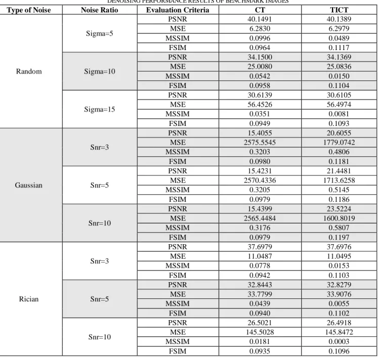
TABLE II
DENOISING PERFORMANCE RESULTS OF BENCHMARK IMAGES
Type of Noise Noise Ratio Evaluation Criteria CT TICT
Random Sigma=5 PSNR 40.1491 40.1389 MSE 6.2830 6.2979 MSSIM 0.0996 0.0489 FSIM 0.0964 0.1117 Sigma=10 PSNR 34.1500 34.1369 MSE 25.0080 25.0836 MSSIM 0.0542 0.0150 FSIM 0.0958 0.1104 Sigma=15 PSNR 30.6139 30.6105 MSE 56.4526 56.4974 MSSIM 0.0351 0.0081 FSIM 0.0949 0.1093 Gaussian Snr=3 PSNR 15.4055 20.6055 MSE 2575.5545 1779.0742 MSSIM 0.3203 0.4806 FSIM 0.0980 0.1181 Snr=5 PSNR 15.4231 21.4481 MSE 2570.4336 1713.6258 MSSIM 0.3205 0.5145 FSIM 0.0979 0.1186 Snr=10 PSNR 15.4399 23.5224 MSE 2565.4484 1600.8019 MSSIM 0.3176 0.5807 FSIM 0.0979 0.1197 Rician Snr=3 PSNR 37.6979 37.6976 MSE 11.0487 11.0495 MSSIM 0.0778 0.0153 FSIM 0.0942 0.1103 Snr=5 PSNR 32.8443 32.8279 MSE 33.7799 33.9076 MSSIM 0.0439 0.0055 FSIM 0.0940 0.1102 Snr=10 PSNR 26.5021 26.4918 MSE 145.5028 145.8472 MSSIM 0.0181 0.0003 FSIM 0.0935 0.1096 REFERENCES
[1] K. Panetta, S. Agaian, J.-C. Pinoli, and Y. Zhou, Image processing algorithms and measures for the analysis of biomedical imaging systems applications, International journal of biomedical imaging, vol. 2015, 2015.
[2] K. Leung, A. Cunha, A. W. Toga, and D. S. Parker, Developing image processing meta-algorithms with data mining of multiple metrics,
Computational and mathematical methods in medicine, vol. 2014, 2014.
[3] E. Abele, L. Holland, and A. Nehrbass, Image acquisition and image processing algorithms for movement analysis of bearing cages, Journal
of Tribology, vol. 138, no. 2, p. 021105, 2016.
[4] S. Ya-Lin and B. Chen-Xi, Research and analysis of image processing technologies based on dotnet framework, Physics Procedia, vol. 25, pp. 2131-2137, 2012.
[5] R. Patil, Noise reduction using wavelet transform and singular vector decomposition, Procedia Computer Science, vol. 54, pp. 849-853, 2015. [6] A. Boyat and B. K. Joshi, Image denoising using wavelet transform and median filtering, in Engineering (NUiCONE), 2013 Nirma University
International Conference on, 2013, pp. 1-6: IEEE.
[7] R. Sivakumar, G. Balaji, R. S. J. Ravikiran, R. Karikalan, and S. S. Janaki, Image Denoising using Contourlet Transform, in 2009 Second
International Conference on Computer and Electrical Engineering,
2009, vol. 1, pp. 22-25: IEEE.
[8] D. Bhonsle, V. Chandra, and G. Sinha, Medical image denoising using bilateral filter, International Journal of Image, Graphics and Signal
Processing, vol. 4, no. 6, p. 36, 2012.
[9] A. B. Hamza and H. Krim, Image denoising: A nonlinear robust statistical approach, IEEE transactions on signal processing, vol. 49, no. 12, pp. 3045-3054, 2001.
[10] A. Dixit and P. Sharma, A Comparative Study of Wavelet Thresholding for Image Denoising, IJ Image, Graphics and Signal Processing, vol. 12, pp. 39-46, 2014.
[11] N. Mehala and R. Dahiya, A comparative study of FFT, STFT and wavelet techniques for induction machine fault diagnostic analysis, in
Proceedings of the 7th WSEAS international conference on computational intelligence, man-machine systems and cybernetics, Cairo, Egypt, 2008, vol. 2931.
[12] T. Bernas, E. K. Asem, J. P. Robinson, and B. Rajwa, Compression of fluorescence microscopy images based on the signal‐ to‐ noise estimation, Microscopy research and technique, vol. 69, no. 1, pp. 1-9, 2006.
[13] R. M. Willett and R. D. Nowak, Platelets: a multiscale approach for recovering edges and surfaces in photon-limited medical imaging, IEEE
Transactions on Medical Imaging, vol. 22, no. 3, pp. 332-350, 2003.
[14] J. B. De Monvel, S. Le Calvez, and M. Ulfendahl, Image restoration for confocal microscopy: improving the limits of deconvolution, with application to the visualization of the mammalian hearing organ,
Biophysical Journal, vol. 80, no. 5, pp. 2455-2470, 2001.
[15] P. V. Lavanya, C. V. Narasimhulu, and K. S. Prasad, Transformations analysis for image denoising using complex wavelet transform, in
Innovations in Information, Embedded and Communication Systems (ICIIECS), 2017 International Conference on, 2017, pp. 1-7: IEEE.
[16] P. Rakheja and R. Vig, Image Denoising using Various Wavelet Transforms: A Survey, Indian Journal of Science and Technology, vol. 9, no. 48, 2017.
[17] M. N. Do and M. Vetterli, The contourlet transform: an efficient directional multiresolution image representation, IEEE Transactions on
image processing, vol. 14, no. 12, pp. 2091-2106, 2005.
[18] P. Hiremath, P. T. Akkasaligar, and S. Badiger, Performance comparison of wavelet transform and contourlet transform based methods for despeckling medical ultrasound images, International Journal of
Computer Applications, vol. 26, no. 9, pp. 34-41, 2011.
[19] E. J. Candès and D. L. Donoho, Ridgelets: A key to higher-dimensional intermittency?, Philosophical Transactions: Mathematical, Physical and
Engineering Sciences, pp. 2495-2509, 1999.
[20] E. J. Candes and D. L. Donoho, Curvelets: A surprisingly effective nonadaptive representation for objects with edges, Stanford Univ Ca Dept of Statistics2000.
[21] J. Xu, L. Yang, and D. Wu, Ripplet: A new transform for image processing, Journal of Visual Communication and Image Representation, vol. 21, no. 7, pp. 627-639, 2010.
[22] J. Krommweh, Tetrolet transform: A new adaptive Haar wavelet algorithm for sparse image representation, Journal of Visual
Communication and Image Representation, vol. 21, no. 4, pp. 364-374,
2010.
[23] M. Ceylan and A. E. Canbilen, Performance Comparison of Tetrolet Transform and Wavelet-Based Transforms for Medical Image Denoising, International Journal of Intelligent Systems and Applications
in Engineering, vol. 5, no. 4, pp. 222-231, 2017.
[24] M. Saha, M. K. Naskar, and B. Chatterji, Wavelet and Curvelet Transforms for Biomedical Image Processing, in Handbook of Research
on Information Security in Biomedical Signal Processing: IGI Global,
2018, pp. 95-129.
[25] P. Jain and V. Tyagi, An adaptive edge-preserving image denoising technique using tetrolet transforms, The Visual Computer, vol. 31, no. 5, pp. 657-674, 2015.
[26] Q. Huang, B. Hao, and S. Chang, Adaptive digital ridgelet transform and its application in image denoising, Digital Signal Processing, vol. 52, pp. 45-54, 2016.
[27] R. Eslami and H. Radha, Translation-invariant contourlet transform and its application to image denoising, IEEE Transactions on image
processing, vol. 15, no. 11, pp. 3362-3374, 2006.
[28] M. Bouhrara et al., Incorporation of Rician noise in the analysis of biexponential transverse relaxation in cartilage using a multiple gradient echo sequence at 3 and 7 Tesla, Magnetic resonance in medicine, vol. 73, no. 1, pp. 352-366, 2015.
[29] P. J. Burt and E. H. Adelson, The Laplacian pyramid as a compact image code, in Readings in Computer Vision: Elsevier, 1987, pp. 671-679. [30] R. H. Bamberger and M. J. Smith, A filter bank for the directional
decomposition of images: Theory and design, IEEE transactions on
signal processing, vol. 40, no. 4, pp. 882-893, 1992.
[31] P. Han and J. Du, Spatial images feature extraction based on bayesian nonlocal means filter and improved contourlet transform, Journal of
Applied Mathematics, vol. 2012, 2012.
[32] J. Staal, M. D. Abràmoff, M. Niemeijer, M. A. Viergever, and B. Van Ginneken, Ridge-based vessel segmentation in color images of the retina, IEEE transactions on medical imaging, vol. 23, no. 4, pp. 501-509, 2004.
[33] V. N. P. Raj and T. Venkateswarlu, Denoising of Poisson and Rician Noise from Medical Images using Variance Stabilization and Multiscale Transforms, International Journal of Computer Applications, vol. 57, no. 21, 2012.
[34] Z. Wang, Z. Li, W. Lin, and C. Liu, Image quality assessment based on improved feature similarity metric, work, vol. 22, p. 24, 2011.
BIOGRAPHIES
MUHAMMET FATIH ASLAN is a research assistant at Karamanoglu
Mehmetbey University (KMU),
Karaman, Turkey. After completing his BSc with a high degree in Selçuk University (SU), Konya, Turkey in 2016, he started to work in Karamanoglu Mehmetbey University in 2017. In 2018, he completed his master's degree at Selcuk University. He is currently a PhD student in Electrical and Electronic Engineering at Konya Technical University. His research interests include robotics, image processing, machine learning and object tracking.
KADIR SABANCI was born in 1978. He received his B.S. and M.S. degrees in Electrical and Electronics Engineering (EEE) from Selcuk University, Turkey, in 2001, 2005 respectively. In 2013, he received his Ph.D. degree in Agricultural Machineries from Selcuk University, Turkey. He has been working as Assistant Professor in the Department of EEE at Karamanoglu Mehmetbey University. His current research interests include image processing, data mining, artificial intelligent, embedded systems and precision agricultural technology.
AKIF DURDU has been an assistant professor with the Eletrical-Electronics Engineering Department at the Konya Technical University since 2013. He earned a PhD degree in Eletrical-Electronics engineering from the Middle East Technical University (METU), in 2012. He received his B.Sc. degree in Eletrical-Electronics Engineering in 2001 at the Selcuk University. His research interests include mechatronic design, search & rescue robotics, robot manipulators, human-robot interaction, multi-robots networks and sensor networks. Dr. Durdu is teaching courses in control engineering, robotic and mechatronic systems.