The response of Asian equity indexes US us macro-economic announcements

(1)

İSTANBUL BİLGİ ÜNİVERSİTESİ

SOSYAL BİLİMLER ENSTİTÜSÜ

FİNANSAL EKONOMİ YÜKSEK LİSANS PROGRAMI

THE RESPONSE OF ASIAN EQUITY INDEXES TO US

MACRO-ECONOMİC ANNOUNCEMENTS

Şaziye KARAÇAVUŞ

114624004

Yrd. Doç. Dr. Deniz İKİZLERLİ

İSTANBUL

2017

(2)

(3)

i

TABLE OF CONTENT

1. INTRODUCTION ... 1

2. REVIEW OF THE LITERATURE ... 3

3. DATA ... 7 4. METHODOLOGY ... 12 5. RESULT ... 14 5.1. Economy of Thailand ... 14 5.1.1. Thailand Result ... 15 5.2. Economy of Taiwan ... 16 5.2.1. Taiwan Result... 17

5.3. Economy of South Korea ... 19

5.3.1. South Korea Result ... 19

6. CONCLUSION ... 24

7. APPENDİX ... 28

7.1. Thailand... 28

7.2. Taiwan ... 31

(4)

ii

7.4. Thailand Good-Bad ... 37

7.5. Taiwan Good- Bad ... 40

7.6. South Korea Good- Bad ... 43

(5)

iii

Abstract

The aim of this study to examine the impact of US macro-economic announcements on Thailand-50, Taiwan-50 and South Korea-50 indexes between 2009-2016. In order to observe this effect, the closing prices of the indexes, the difference between the expectations of 6 types of macro-economic announcements and the actual released data have been used. In the conducted analysis, it has been observed that each index reacted to different macro-economic news. Thailand-50 index is found to be affected from the consumer price index and gross domestic product announcements, Taiwan-50 index is only affected from gross domestic product announcement and South Korea-50 index is found to be only affected from non-farm payrolls announcements. In order to take more detailed results in the next step, we have divided the surprise variables into two groups as positive and negative variables and analyzed them. While Thailand and Taiwan indexes have been affected from the announcements which are the same in the previous analysis, South Korea index has only been affected from the unemployment rate.

Keywords: Macro-economic announcement, emerging markets, closing price, surprise price.

(6)

iv

Özet

Bu çalışmanın amacı; 2009-2016 yılları arasında ABD makro ekonomik duyuruların, Tayland-50, Tayvan-50 ve Güney Kore-50 endeksleri üzerindeki etkisini incelemektir. Bu etkiyi gözlemlemek için, endekslerin kapanış fiyatları ve 6 makro ekonomik duyuruların beklentileri ile açıklanan gerçek değerleri arasındaki fark ile elde edilen sürpriz veriler kullanılmıştır. Yapılan analizde, her bir endeksin farklı makro-ekonomik haberlere tepki gösterdiği gözlemlendi. Tayland-50 endeksi, tüketici fiyat endeksi ve gayri safi yurtiçi hasıla duyurusundan etkilenirken, Tayvan-50 endeksi sadece gayri safi yurtiçi hasıladan etkilenmekte. Güney Kore-50 endeksi ise tarım dışı istihdam duyurusundan etkilenmektedir. Bir sonraki adımda daha ayrıntılı sonuçlar almak için, sürpriz değişkeni pozitif ve negatif olmak üzere iki gruba ayırdık ve analiz ettik. Tayland ve Tayvan endeksleri önceki analizde aynı verilerden etkilensede, Güney Kore endeksi yalnızca işsizlik oranından etkilenmiştir.

Anahtar kelime :Makro-ekonomik duyurular, gelişmekte olan piyasalar, kapanış fiyatı, sürpriz fiyat.

(7)

1 1. INTRODUCTION

Finance market has always been in connection with the released macro-economic announcements in either a scheduled or a non-scheduled form. Then the question of how the regular and scheduled releases of the macro-economic announcements in the market affect the forward looking beliefs and the investors‟ preferences comes to the mind. Almost all the interpreters make their predictions related to the scheduled macro-economic announcements before the relevant data come. These expectations stand as a guideline for the investments of the traders. According to Market efficiency hypothesis, expected information should already be incorporated into the prices, only new information can affect asset values. On this basis, following the announcements, market participants try to price the assets based on the unexpected component of the news.

Almost all studies in this strand of literature have the same subject, which is the impact of the news. These announcements are related to the firms and the economy, but they are not periodical. Moreover, it is not known in which time periods these announcements will be released. Besides, all investors do not have the equal opportunities of being informed about the upcoming news. When this is compared with the past, there are various sources from the trading platforms, the questionnaires of the trading platforms to the media channels focusing on the economic developments at this point. In this way, millions of people are informed about them, thus their forward looking beliefs and preferences about trading or investment are formed.

Mostly, investors‟ reactions to the expectations for the macro-economic announcements are supported by the efficient market hypothesis. The effects of the announced data on the stock market prices are independent from the previous stock

(8)

2

prices. However, some traders and investors consider the stock market prices as repetitive. We are interested in the effect of new information on price movements. We try to find an answer of whether new information has an influence on stock returns or not by employing appropriate tests.

The purpose of this study is to determine how the Asian stock market responds to the release of the available global economic news in other words the US macro-economic news. Macro-macro-economic news can either be scheduled and non-scheduled. However, what we examine here will be the scheduled macro-economic news.

The reason behind choosing US market is its important role in the world stock market and its higher level of development. We have chosen the Asian stock market as the market we expect to be affected. Asian countries examined in this study are: South Korea, Thailand and Taiwan. The reasons why we have chosen the Asian stock markets are their economic structures and their time difference with the US.

The stock market‟s reaction to the current macro-economic data is different when it is compared to the previous ones. This means that the investors‟ perspectives about the released data and its order of importance have changed. The reason for the other difference is that the data now include the politics and the international relations and these components are responded by the market.

Asian stock market prices have been thought to change rapidly due to the macro-economic news from US so this study aims to find whether this is the case for the changing prices. Three steps have been employed to facilitate the examination. In the first step, a connection has been set up between the economic structures of the chosen countries and the macro-economic variables. In other words, we ask which variables the assets would react more. In the second step, the surprise portions of the scheduled macro-economic announcements have been calculated. Finally, we test whether these surprise values have any effects on the asset values of these countries. The common macro-economic variables chosen according to the economic structures of these three

(9)

3

countries: The macro-economic variables of US are listed as the Consumer Price Index (CPI), Non-farm payroll employment (NFP), Unemployment rate (UNEM), industrial production (INDP), gross domestic product (GDP) and initial jobless claims (INJC).

The data in this study obtained from Bloomberg and Money Market Services (MMS) are the real time data related to expectation and realization. The period was from 2009 to 2016. Investors need some time to process news. On this basis, intraday data might not be consistent with the idea. Therefore, the reactions of stock markets to macro-economic announcements are examined on a daily basis.

The study consists of three parts: first; the review of the relevant literature, second, the methodology used for the empirical frame work and as a third, the study discusses the results and the final part provides the conclusion.

2. REVIEW OF THE LITERATURE

The previous studies have examined the effect of the macro-economic news on the stock prices, however, all of them have handled this subject in terms of economic conditions, monthly/daily/hourly data and developed/emerging markets. The researchers conducted by Fama (1969), Waud (1970), Castanias (1979), Schwert (1981), Pearce and Roley (1985), Hardouvelis (1987), CulterPoterba (1989) etc. are about the impact of the macro-economic announcements on the market prices.

Fama has conducted researches about the reactions to the stock split announcements via using the data on a monthly basis. When the stock split announcements are reflected in the stock price, they cannot distinguish the expected from the unexpected (1969). The change in the interest rate immediately and significantly creates a negative response to stock price, but Waud (1970) said that it cannot be tested with the incomplete data which can be described as more than one day.

(10)

4

In multi-factor asset pricing models, many variables are observed to have effects on the future investment opportunities or the level of consumption. For the risk averse economy, non-diversifiable risk factors should be taken into consideration by the investors so that they can earn the risk premium (Ross 1976). Since the macro-economic variables change simultaneously, they may cause many risk factors. As a result of this, many firms can be affected by the cash flows and the risk adjusted interest rate.

Castanias (1979) found a short term deviation in the stock prices during the days before and after the macro-economic announcements and this can be interpreted as the representation of the new information emerging. He also reported that this deviation could not be predicted as expected or unexpected because the macro-economic announcements were scheduled.

Different results have been found in the conducted research from the early 1980s to 1990s. Schwert (1981) preferred to use an unpredictable inflation rate instead of the announced rate. He found that the daily reaction of the stock prices to the inflation news was weak and slow from 1953 to 1978. As a result of this research, he decided that this situation had some conflicts with the efficient market hypothesis because the announcement of inflation did not have an immediate effect on the stock prices. Pearce and Roley (1983), on the other hand, found that the efficient market theory was coherent with the weekly announcements about the money stock. The original research topic was revised along with the unpredictable changes in the macro-economic news. No impact on the industrial production and the unemployment rate was observed by Pearce and Roley (1985). A negative impact was found on the stock price and what created this impact was the upcoming monetary policy announcements according to Schwert (1981), Pearce and Roley (1985) and Hardaouvelis (1987). When the inflation rate is different from the expected, it creates a limited effect on the stock price. However, Hardouvelis (1987) stated the fact that the actual rates of the

(11)

5

unemployment rate, the trade deficit and personal income data were different than the expected created a crucial impact on the stock prices and he found out the primary impact of the monetary news. On the other hand, the data on an hourly basis was used by Jain (1988). He stated that the monetary and inflation surprises were significant. Culter, Poterba and Summers (1989) explored the alteration among the fifty largest daily S&P 500 index returns, when the important announcements were released from 1946 to 1987. Thus, they observed a negative impact on the common stock caused by the inflation rate.

Haugen, Talmor and Torus (1993) conducted many studies on market price, volatility and economic events. The result of these studies is that a negative response was observed from the market price and it did not have parallels with the volatility changes, but the used data set caused an increase in the volatility for 28 out of 217 variables and a decrease in the volatility for 18 out of 224 variables.

On the other hand, McQueen and Roley (1993) had a research about the impact of the macro-economic news such as the monthly industrial production index on the stock market with a business condition. If the economy of a country was strong, the stock price and the unemployment rate would be lower, while the industrial production would be higher. Otherwise, the stock prices would be higher for the same surprise news. Other economic news about the topics of trade deficit, inflation and money supply gave a negative reaction to the stock price when it was compared with the different state of the economy. Even so, they could only explain a small subdivision of the daily S&P index variance.

Jones, Lamont and Lumsdaine (1998) and Christiansen (2000) conducted studies about the impact of the producer price index and the employment rate on Treasury bond market volatility. They detected a significant increase in the bond market volatility on the announcement days, while they did not observe this increase in the price immediately, on the other hand.

(12)

6

A group of researchers examined the impact of U.S. macro-economic announcements on the stock markets of 12 foreign countries. During the research, Conolly and Wang (2003) found a correlation among USA, UK and Japanese stock markets, but this correlation could not explain the macro-economic fundamentals. Moreover, another researcher Bialkowskia (2006) determined that there was an impact of the US macro-economic news on the stock markets in the UK, Germany and Japan, while there was no impact on the other stock markets.

The study conducted by Kim Et Al. (2004) has different points when it is compared to the others. They examined the impact of differences between the expectations of the market and the market price figures. They showed that the effect of the producer and consumer price announcement on the stock was higher. Moreover, they discovered that the market volatility showed an attribute of the increase in some of the announcements by some classes while it showed an attribute of decrease for others.

Andersen, Bollerslev, Diebold and Vega (2005) used the high frequency data and they found an asymmetric pattern similar to the pattern of Haugen, Talmor and Torus. However, the stock markets gave stronger reactions to the news announced unexpectedly. They took this fact, as a base for the competitive effects of the cash flows and the interest rates on the asset evaluations.

Nikkinen (2006) analyzed the behavior of the volatility in several regions around the world involving The Czech Republic, Hungary, Poland, Slovakia and Russia by using monthly data for whether the important scheduled US macro-economic announcements had an impact on the stock market in these regions of the world or not. Another study conducted by Nikkinen, found the US macro-economic news affected European and Asian stock markets. On the other hand, the same news did not have the same impact on Latin American and the transitional markets. Then the study

(13)

7

of Nikkinen showed us these markets as a group which was not affected by US macro-economic announcement.

Albuquerque and Vega (2009) conducted their research in a different way. Since it is not easy to find the impact of U.S. macro-economic news on the stock prices of the large foreign economies, they had a research on smaller markets such as Portuguese. This approach helped them to find out the impact of the U.S. macro-economic news on stock market.

Birz and Lott (2011) had a different perspective about the impact of macro-economic news due to the lack of evidence about the fact that the stock prices did not respond to all released macro-economic data, which was started by the previous studies. They examined the reason. Some macro-economic data were important for the asset price such as the unemployment rate, the non-farm payroll employment and because of this, the impacts of the most analyzed economic factors did not give statistically and economically significant results. Another reason was that some important macro-economic data were more evaluated by the traders. In addition to this, there was a surprise macro-economic data. This showed us the differences between expectations and the released macro-economic data.

3. DATA

Every stock market in the world has a specific time period. There are lots of macro-economic data coming from different countries at any time between the transaction periods. The arrival time of the data may be at any time, which is different from the announced time because of time offset. For instance, the macro-economic data announced at 8:30 am in the US, may reach to Turkish stock market at 16:30 pm arriving US macro-economic announcements may not have the same impact on the Turkish stock market because between 9:30 and 16:30, the Turkish stock market may

(14)

8

be affected by other economic news. The most important answer for why we have chosen the Asian market in our research is the time difference.

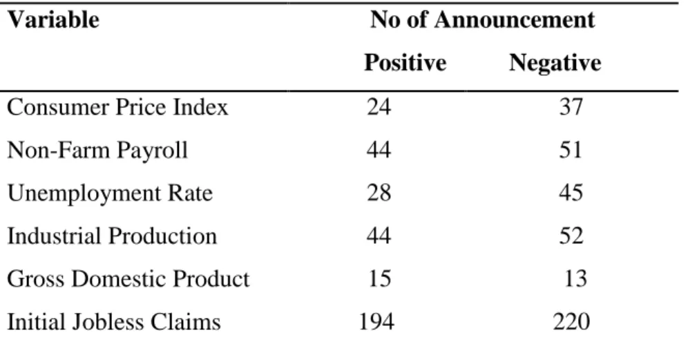
The time difference between the US, and Asian countries (South Korea, Taiwan, and Thailand) are approximately thirteen hours. Because of the time difference, the Asian stock market firstly affected by the US macroeconomic data. The closing prices of the indices are used when determining the indices returns. We can observe the impact of the surprise macro-economic announcements on stock markets by following this path. After examining the effect of all surprise variables in the first stage, we will see their effects in detail via separating them as positive and negative. The positive and negative surprises for each US variable have different meanings. Let‟s exemplify whether the positive/negative variables are good or bad for the economy.

If we need to tell it more clearly, we will examine separately whether each variable is less or more than the expectations. The fact that the Consumer Price Index variable is more than the expected causes the surprise variables to be found more than expected. This means that inflation has increased more and this has a bad meaning for the economy. The fact that the Non-farm Payroll surprise variable is positive means that the real value is higher than the expectation. In terms of economy, the increase in the employment is a good sign. If the surprise of the unemployment variable is positive, it is bad for economy, because unemployment increase is bad. If the industrial production variable is positive, this means that the production has increased more than the expected. The increase in the production affects the economy in a good way. The fact that the positive Gross Domestic Product variable is good news for the economy, which means the increase in the growth. If initial jobless claim‟s variable result is positive, this means unemployment rate increases and this really bad for the economy.

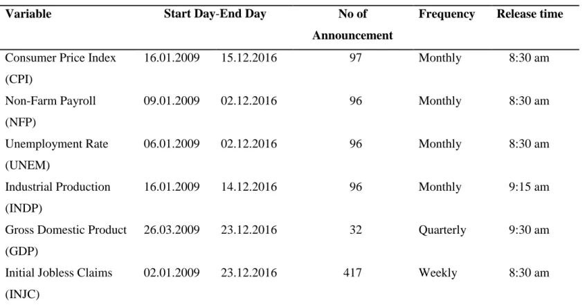
We use announcements only from US which are as follows: Consumer Price Index, Non-Farm Payrolls data, Unemployment Rate, Industrial Production, Gross Domestic

(15)

9

Product and Initial Jobless Claims. The frequency and times of releases of macroeconomic data are given in the table below. Asian stock markets for analysis are as follows: The end-of-day prices of Thailand-50 index (SET-50), Taiwan-50 index (TWSE-50) and South Korea index (KOSPI-50) were used. The study period was from 2009 to 2016. The data used were acquired from the Bloomberg trading platform.

(16)

10

Variable Start Day-End Day No of

Announcement

Frequency Release time

Consumer Price Index (CPI) 16.01.2009 15.12.2016 97 Monthly 8:30 am Non-Farm Payroll (NFP) 09.01.2009 02.12.2016 96 Monthly 8:30 am Unemployment Rate (UNEM) 06.01.2009 02.12.2016 96 Monthly 8:30 am Industrial Production (INDP) 16.01.2009 14.12.2016 96 Monthly 9:15 am

Gross Domestic Product (GDP)

26.03.2009 23.12.2016 32 Quarterly 9:30 am

Initial Jobless Claims (INJC)

02.01.2009 23.12.2016 417 Weekly 8:30 am

Table 1: This table, in the first column, shows macro-economic variables that were analyzed. The second column shows the beginning

and ending dates for each macro-economic variable. The third column shows the number of announcements during the period. The fourth column shows the frequency of the macroeconomic announcement. The announcement time in the last column belongs to US time.

(17)

11

Variable Min Max Mean Standard Deviation

Consumer Price Index -3.763554373 2.258132624 -0.147438213 0.855421845

Non-Farm Payroll -1.972342406 2.838248828 -0.026725507 1.004797314

Unemployment Rate -3.32000767 1.992004602 -0.283583988 1.017645949

Industrial Production -2.802924016 2.262911133 -0.131520995 0.902679879

Gross Domestic Product -3.627723571 2.308551363 -0.030918099 1.12553015

Initial Jobless Claims -4.45998992 3.752055012 -0.005673099 0.95354378

Table 2: First column shows the min. value of the surprise variables, the second column shows their maximum values, the third one shows the average values of all surprise variables and last column gives the standard deviations of these surprise variables.

Variable No of Announcement

Positive Negative

Consumer Price Index 24 37

Non-Farm Payroll 44 51

Unemployment Rate 28 45

Industrial Production 44 52

Gross Domestic Product 15 13

Initial Jobless Claims 194 220

Table 3: The columns give respectively the number of positive and negative results of the surprise values.

(18)

12 4. METHODOLOGY

Regression analysis of the statistical model was used for our research. It is related to the description and assessment of the relationship between a given variable, in other words the dependent variable, and one or more other variables, known as the explanatory variables.

The regression model is: r_t   * _t _t (1)

The function shows us how r is influenced by the changes in macroeconomic _t

variables

t

r : Dependent variable

: Surprises in macroeconomic announcements in other words “unexpected portion of the announcements”

α: Intercept β : Slope

ε: Random error term

The return is calculated by subtracting the logarithmic values of the closing price of the previous day from the present day; n(e_t_₁)n(e_t).

Calculation formula for the value of surprise is:

value -

(2)

i i

i

Actual Forecast value Surprise



(19)

13

The dependent variable gives response, according to the change of the explanatory value. The regression analysis gives the answer of whether the response is significant or not.

The days on which the selected macro-economic data during the specified years were obtained through the Bloomberg platform. Two different values from the selected macro-economic variable were required. One of them was the expectation survey value for the market, and the other was the actual released value. The surprises in macroeconomic announcements are calculated as the difference between the actual data value and the market expectation value. We then also standardize the surprises by dividing each announcement surprise by its sample standard deviation, following Balduzzi et al. (2001). Explanatory variable has been employed in this way.

In order to obtain true estimates in the regression analysis we employ same day return for the announced macroeconomic data. This rule could be applied, if the selected countries were in the same time zone. However, the US and Asian countries are in different time zones. The time difference between the US and South Korea, Taiwan and Thailand are approximately thirteen hours. For instance, the CPI data is explained on t day in the US at 8:30 am. The time of the releases of the US data equal to time zone, which is t1 day of South Korea and Taiwan at 9:30 pm. The time of the release of US data is equal to the night time in South Korea, Taiwan and Thailand which is at 9:30 pm on t1 day. As shown in this example, if the day is selected as day t for the releases macro-economic data, the return will be the day t1 for the Asian markets and this should be selected to examine the effects of these data. Actually, an advantage for research is the time differences between the selected countries. Because of time differences, Asian stock market is affected by the US macro-economic data firstly. Local stock market returns of South Korea, Taiwan and Thailand are regressed separately on US macroeconomic surprises variable. The

(20)

14

regression results will determine whether the established hypothesis is significant or not.

Equity responses to the unexpected component of macroeconomic announcements may be different depending on whether the news is positive or negative. Therefore, rather than estimating equation (2), we extend our model allowing equity responses to depend on whether the news surprise is good or bad.

Responses of equity indices to macroeconomic announcements conditional on the sign of the news:

* * * * (3)

t BAD GOOD BAD t GOOD t t

r    BAD   GOOD  

BAD and GOOD are dummy variables for bad news and good news respectively. BAD = 1 if the surprise at time t is „bad‟, and zero otherwise;

GOOD = 1 if the surprise at time t is „good‟, and zero otherwise. All other variables are defined as in Equation 1.

5. RESULT

Before writing up the results it may be useful to give some background information about analyzed countries‟ economies.

5.1. Economy of Thailand

As a result of the changes that took place until 1998, Thailand had an outstanding economy in the South East Asia. Thailand‟s economy had a transformation from a traditional economy depending on agricultural exports to an economy depending on the import substitution in the 1970s. While it was a developing economy depending on the textile and ready-to-wear production during the 1980s, the export of the

(21)

15

technologic products such as the computer accessories and the parts of the motor vehicles was on the rise during the 1990s. The relation between Thailand‟s currency Baht and the indexation to the US dollar officially began in 1990.

Thailand is the only country exporting to the industries such as textiles, technologic products and automotive. Those who have this quality are expected to be influenced by the changes in other countries' economies, as well. At this point if we are going to mention other countries‟ economies, the first country that comes to the minds is the United States. The US holds the top place in the list of developed countries and the country has the highest amount of the economic relations with all the countries around the world. The impact of the US macroeconomic variables (CPI, NFP, Unemployment Rate, Industrial Production, GDP and initial job claims) on Thailand‟s stock market was investigated. When the effect of each economic variable is examined separately, the results are as the following in Thailand-50 index.

5.1.1. Thailand Result

As Thailand's revenue source largely comes from the exported products, it is expected to be affected by the macroeconomic changes that take place in the other countries. In order to show this effect in the analysis, the end-of-day prices of SET-50 index between 2009 and 2016 were employed. In the regression model, a confidence interval of 10% is used.

The result obtained in the regression model using 10% confidence interval is as the following: the consumer price index and the gross domestic product announcements are proved to have an effect on the SET-50. A country that exports in the fields such as textile, technologic products and automotive would be expected to be affected from the variables of CPI, GDP and NFP. The analysis made has met some of our expectations. We can interpret that Thailand‟s export rates change as the people‟s purchase power and, in accordance, purchase requisition change. It has been observed

(22)

16

that the surprise CPI and GDP variables announced by the USA, which has a high level of consumption rates, affect SET-50 index. Moreover, the surprise NFP variable has also been expected to be affected and we considered that the consumption demand would change as the employment level changed. However, the analysis has shown that this is not significant.

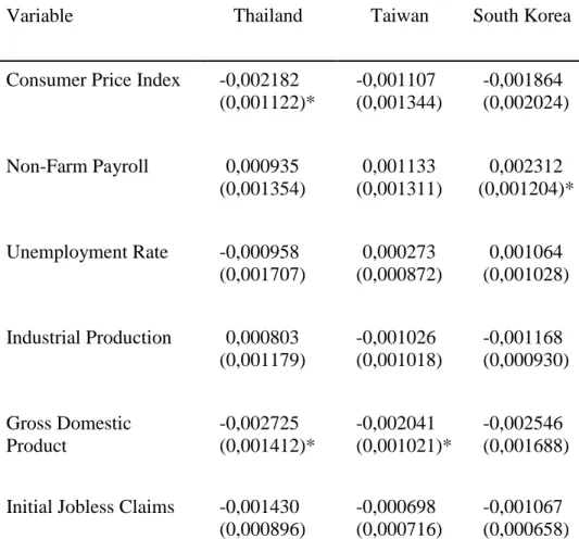
According to this hypothesis, while the consumer price index and the gross domestic product announcements are found to have significant effect on Thailand stock market, non-farm payroll, unemployment rate, industrial production and initial jobless claims announcements are not found to have significant effect.

The results of the first hypothesis are mentioned above. Now in our second hypothesis, we will examine in detail the effects of the surprise variables by separating them as positive and negative. In this analysis, our results have not been so different. Consumer price index and gross domestic product values are significant. However, in this analysis we could see whether the bad variable or the good variable is significant. Good CPI surprise variable means the actual data has come less than the expectation. In the conducted analysis, the good CPI surprise variable has been significant, bad CPI surprise variable has been insignificant. We can interpret this like this: The decreased inflation means that people can buy more or save more money with the money they have. In both situations, Thailand-50 index has been affected positively. For the GDP, the bad surprise variable has been significant. When GDP gets smaller, people‟s power to purchase decreases. This situation affects the Thailand-50 index negatively.

5.2. Economy of Taiwan

Taiwan has been an independent country since its separation from People‟s Republic of China in 1949. In the past, the most of Taiwan‟s economy was depending on the agricultural products. However, a big turning point was observed with the

(23)

17

developments in the industry and the urbanization. With this change in the economic field, the country rapidly developed itself.

During the Korean War in 1954, an alliance agreement was signed with the ADB. With this agreement, the country began to develop with the internal and external influences. More of the agricultural products produced in the country began to be exported. The foreign exchange gain from this export was used as a source for the developments in the industry. After the 1990s, the imported goods were converted into the cheap consumer goods using the developing industry. With the export of the cheap consumer goods, there has been a great improvement in the economy of Taiwan.

Today, Taiwan is involved in the ranking list of the developing countries. Taiwan's exports are connected to other countries; in this case Taiwan is thought to be influenced by the changes in other country's economies, as well.

The analysis of the paper aims to tell how Taiwan has given reaction to these changes. The impact of the US macroeconomic variables (CPI, NFP, Unemployment Rate, Industrial Production, GDP and initial job claims claims) on Taiwan‟s stock market was investigated. The results of each economic data examined separately are shown in Taiwan-50 index.

5.2.1. Taiwan Result

Once Taiwan was a small country depending on agriculture, but it has been creating an economy based on the exports using science and technology. The imported raw materials are processed, turned into the cheap consumer products and exported the other countries. In this way, it has been opened to the outside and has announced its name to the world. Taiwan, whose productions and sales are depending on the foreign countries, is expected to be influenced by the changes in other economies. To observe

(24)

18

the reactions to the macro-economic data announced out of the USA, the closing prices in TAIWAN-50 index will be examined.

The regression analysis is performed using a confidence interval of 10%. We find that Gross Domestic Product surprise announcement has an effect on the TWSE-50 index. We can interpret why this variable is significant for TWSE-50 index as Taiwan‟s dependency to outside world to buy raw materials and sell the processed products. In order to sell the products to other countries, other countries need to grow in a healthy rate and their purchase demands need to increase. We would expect that a country with such an economy affected from CPI and unemployment rate variables. The purchase power, in other words, the inflation is a factor that affects the purchase demand, but we have seen that it is insignificant for the TWSE-50 index. Furthermore, when unemployment rate increases, it influences the consumption demand. However, we have observed that it is not significant for TWSE-50, either. According to this hypothesis, while the coefficient on Gross Domestic Product surprise data is found to be significant, the coefficients on consumer price index, non-farm payroll, unemployment rate, industrial production and initial jobless claims surprise data are not found to be significant.

The results above belong to our first hypothesis. In order to interpret these effects in detail, we have separated the surprise data as positive and negative. Our second hypothesis‟s result is not different from the first one. While bad GDP variable is significant, good GDP surprise variable is insignificant. When the growth gets slower, this affects the economy negatively and the consumer behaviors change. We see a situation in which the expenditures are decreased. Taiwan-50 index has been affected from this case.

(25)

19 5.3. Economy of South Korea

South Korea, which has achieved a steady growth since 1960, is now in the ranking list for the developed countries. South Korea, the world's 6th largest exporter and 7th importer, was once an undeveloped agricultural country with no natural resources when it comes to its economic history. The economic development process of South Korea was full of difficulties.

From 1910 to 1945, Korea was under the invasion of Japan. Only after the end of World War II, Korea did become an independent country. During 1950s, the Korean War took place and Korea was divided into two countries as southern and northern as a result of this war. Later, General Park Chung Hee, who came to the country in 1961, helped the country reach its current status.

In order to be able to take a place in the world economy, South Korea aimed to develop its industry first, then to grow in the field of science and technology. For this purpose, a great level of importance has been given to the field of education so that the country can fulfill its objects. South Korea, one of the developed countries, is investigated to see the reactions of the US, another developed country, to macroeconomic data. The impact of US data (CPI, NFP, Unemployment Rate, Industrial Production, GDP and initial job claims claims) on South Korea‟s stock market was investigated. When the effect of each economic data is examined separately, the results are as in the following on South Korea-50 index.

5.3.1. South Korea Result

South Korea, one of the fastest growing economies of the last 30 years, keeps up its economic status with its export volume. This country which was known as a small agriculture country before has become an industrial leader by using science and technology, and today it is one of the most developed industrial countries. Although South Korea is a developed country, its economy depends on its export volume.

(26)

20

Therefore, the economic status thought to be influenced by economic changes in other countries. The South Korea-50 index between 2009 and 2016 is analyzed to find out its effect. This analyzing process is performed in by using the end-of-day prices of KOSPI-50 index and a confidence interval value of 10% will be used for regression

According to the established hypothesis, the regression results for a 10% confidence interval are as follows: non-farm payroll surprise data appear to have an effect on the KOSPI-50 index. We can interpret why this variable is significant for KOSPI-50 index as: Listed as the world‟s 6th biggest exporter thanks to its global brands, South Korea‟s economy is naturally affected positively or negatively depending on the consumption demand coming from the other countries. Non-farm payroll data gives us how many people are employed in the USA except out of agriculture. Employment means that people earn money and spend their money in return. Some of these expenditures may be consumptions, while the others are investments. For example, the increase of consumption drives South Korea to produce more and improve its economy. At the same time, a country with a stronger economy attracts foreign investors. A country showing export skills would be expected to get affected from GDP variable coming from the US. It can be foreseen that the countries consumption and investment demands increase as their growth rates increase. However, we have observed in the analysis conducted for South Korea that the growth is insignificant. According to this hypothesis, the surprise component of the non-farm payroll announcements is found to be significant while the consumer price index, unemployment rate, industrial production, gross domestic product and initial jobless claim announcements are not found to have significant effect.

From the results of the first hypothesis we mentioned above, we want to achieve more detailed results. Thus, we have separated the surprise variables as positive and negative. Within this separated analysis, Thailand and Taiwan have been significant

(27)

21

for the same variables, while different variables have been significant for South Korea. Bad unemployment rate surprise variable has been significant. If we need to interpret that the economy is not in a good mood where unemployment is high and it means little expenditure for the workers, South Korea-50 index is affected.

(28)

22

Variable Thailand Taiwan South Korea

Consumer Price Index -0,002182 (0,001122)* -0,001107 (0,001344) -0,001864 (0,002024) Non-Farm Payroll 0,000935 (0,001354) 0,001133 (0,001311) 0,002312 (0,001204)* Unemployment Rate -0,000958 (0,001707) 0,000273 (0,000872) 0,001064 (0,001028) Industrial Production 0,000803 (0,001179) -0,001026 (0,001018) -0,001168 (0,000930) Gross Domestic Product -0,002725 (0,001412)* -0,002041 (0,001021)* -0,002546 (0,001688)

Initial Jobless Claims -0,001430 (0,000896)

-0,000698 (0,000716)

-0,001067 (0,000658)

Table 4: The results columns show the coefficients and standard errors in () of the estimated responses of the three Asian stock market Index to US macroeconomic announcements. *indicates significance at the %10 level.

(29)

23 Variable Thailand Good Bad Taiwan Good Bad South Korea Good Bad

Consumer Price Index -0,003386 (0,001757)* -0,000362 (0,00294) -0,001987 (0,001373) 0,000225 (0,003445) -0,001176 (0,001966) -0,002903 (0,006233) Non-Farm Payroll 0,001119 (0,002569) 0,000759 (0,002850) -0,001107 (0,002552) 0,003270 (0,002261) 0,002552 (0,001761) 0,001761 (0,002266) Unemployment Rate -0,000494 (0,001632) -0,001867 (0,005299) -0,000508 (0,001297) 0,001802 (0,002646) -0,001754 (0,001392) 0,006581 (0,003040)* Industrial Production 0,004174 (0,003161) -0,001675 (0,002255) -0,000653 (0,002736) -0,001300 (0,001480) -0,001667 (0,002688) -0,000801 (0,001806) Gross Domestic Product 0,000540

(0,003631) -0,004912 (0,02022)* 4,6E-05 (0,002505) -0,003441 (0,001326)* -0,001483 (0,003316) -0,003258 (0,002429) Initial Jobless Claims -0,003440

(0,002685) 0,000248 (0,001238) -0,002328 (0,001790) 0,001790 (0,000859) -0,001096 (0,001945) -0,001042 (0,001092) Table 5: The results columns show the coefficients and standard errors in () of the estimated responses of the three Asian stock market Index

(30)

24 6. CONCLUSION

When comparing present with the past, it is seen that the technology has developed in every field over the years. Financial markets are affected by the development of technology. Scheduled or non-scheduled macroeconomic announcements and the financial markets are in a constant interaction. These announced macro-economic announcements are transmitted to the tens of thousands of investors very quickly, thanks to the developing technology. Accordingly, the market expectations of the investors are changing very quickly.

In this study, the reactions of financial markets have been examined by means of focusing on the difference between the expected values of the scheduled announcements and their actual values. The scheduled macro-economic announcements used in this study are from the US. The reason for the choice of the US can be explained as: the level of development and having a major role in the world stock market. The stock market, which is expected to be affected by these announcements, is the Asian countries such as; Thailand, Taiwan and South Korea. The reason for choosing the stock markets of Asian countries is due to the time difference. To summarize with an example given in the data section of the study: the macro-economic data announced at 8:30 am in the US, may reach to Turkish stock market at 16:30 pm. The macro-economic data coming from the US may not have the same impact on the Turkish stock market because between 9:30 and 16:30, the Turkish stock market may be affected by other economic news. There is about a thirteen-hour difference between Asia and the US. This means that macroeconomic data released from the US on t day is arriving to Asian markets in t1days. With this, more accurate results have been achieved.

The selected macro-economic data of the US for analysis are: Consumer Price Index, Non-farm Payroll, Unemployment Rate, Industrial Production, Gross Domestic

(31)

25

Product and Initial Jobless Claims. Asian stock market data used for analysis are: The end-of-day prices of Thailand-50 index (SET-50), Taiwan-50 index (TWSE-50) and South Korea index (KOSPI-50). The study period was from 2009 to 2016.

According to the hypothesis; assuming that the US macro-economic announcements, which are different from the expectations, are found to have effect on the Asian stock market. The stock markets of these countries are examined separately. In our second hypothesis, we have separated the variables as positive and negative ones. Later, we made an analysis separately for each country. With this, we have a more detailed result pattern than the first analysis. Regression analysis is performed using a confidence interval of 10%.

These three countries are export oriented countries, but each country reacts differently to different macroeconomic announcements. For example, when looking at the results of regression analysis for Thailand, we find that while consumer price index and gross domestic product announcements are found to be significant; non-farm payroll, unemployment rate, industrial production and initial jobless claims announcements are not significant. In a similar vein, when we look at Taiwan‟s results we see that while gross domestic product data are significant, consumer price index, non-farm payroll, unemployment rate, industrial production and initial jobless claims data are not significant. As a final, when looking at the results of regression analysis for South Korea we can see that while non-farm payroll are found to be significant, consumer price index, unemployment rate, industrial production, gross domestic product and initial jobless claims data are not significant.

In our second analysis for more detailed results we have found these: For example, it is not different for Thailand compared to the first analysis, but we have understood that good/bad surprise variables give opposite reactions. Good Consumer Price Index surprise and Bad Gross Domestic Product surprise variables are significant, while Bad Consumer Price Index surprise and good Gross Domestic Product surprise

(32)

26

variable are insignificant. For our second country Taiwan, the situation was the same. Bad Gross Domestic Product surprise variables are significant inTaiwan-50 index. The first analysis and the second analysis have the same results, but with a single different. Now we show that good/bad surprise variables have opposite reactions. Bad GDP surprise variable is significant while Good Gross Domestic Product surprise variable is insignificant. We have found that for Thailand and Taiwan‟s indexes, the US variables are significant. However this is not the same for South Korea. In the analysis made without separating the surprise variables in South Korea, non-farm payroll variable is significant while bad unemployment rate variable is significant in the analysis without separating the variables as positive/negative. This means the surprises create different reactions on South Korea-50 index when they examined depending on whether they are separated or not.

We can interpret the results we have found as: The US wants the inflation rate increase according to today‟s economic conditions. However the inflation under the expectations shows that the US is in the recuperation period after the crisis and the necessary actions to increase the interests have not been taken. We have found that only Thailand-50 index has reacted when the CPI variable is below the expectations in the US. We can explain this in two simple ways. Thailand is an exporting country because the expected inflation rate in the USA is low and most of its operations are with the US, so Thailand-50 index reacts with the expectation that it cannot sell products to the US. However, we would have expected to see this effect for Taiwan and South Korea. After the CPI was announced below the expectations, the funds in the US may have preferred Thailand for the hot money investment with the expectations that the economy was not going well and FED would not increase the interest rates.

After the crisis the US experienced, the other variable it wants the increase in is NFP because it is foreseen that FED will increase the interest rates when the unemployment decreases and the inflation increases due to that. Out of the countries

(33)

27

we have chosen, only South Korea has reacted to this variable. The reason can be explained as: It cannot see the NFP variable as the key point in order to survive from the damages in the economy after the crisis. ın Thailand and Taiwan indexes, we can say that NFP variable has not the number one importance. However, in the more detailed second analysis, we have seen that the results are different for South Korea. South Korea-50 index has been seen as sensitive to the unemployment variable, which came higher than the expectations. We can explain this as the importance list more specifically prepared. Within these insights, we can say that South Korea can have hot money and investment. The fact that the GDP of the US came lower than the expectation shows that the things are not going well for the US. We can say that the exporting country Thailand and Taiwan‟s stock markets can be affected negatively from this with the expectation that the sales to a deteriorating country will decrease. If we think that South Korea has a value added production structure and has an easier access to the developed capital markets, we can assume that the effect will be so low that it cannot be observed clearly.

As a result, in a global economy under the effect of good and capital markets, the same news may have different results in the countries with similar economies due to the differences among the countries.

(34)

28 7. APPENDİX

7.1. Thailand

Dependent Variable: CPI_RETURN Method: Least Squares

Date: 03/30/17 Time: 19:39 Sample (adjusted): 1 97

Included observations: 97 after adjustments

HAC standard errors & covariance (Bartlett kernel, Newey-West fixed bandwidth = 4.0000)

Variable Coefficient Std. Error t-Statistic Prob.

C -0.001591 0.001349 -1.179420 0.2412

CPI_SURPRISE -0.002182 0.001122 -1.944204 0.0548 R-squared 0.023590 Mean dependent var -0.001269 Adjusted R-squared 0.013311 S.D. dependent var 0.012216 S.E. of regression 0.012134 Akaike info criterion -5.965150 Sum squared resid 0.013988 Schwarz criterion -5.912063 Log likelihood 291.3098 Hannan-Quinn criter. -5.943684 F-statistic 2.295144 Durbin-Watson stat 1.781429 Prob(F-statistic) 0.133099 Wald F-statistic 3.779929 Prob(Wald F-statistic) 0.054829

Dependent Variable: NFP_RETURN Method: Least Squares

C -0.000134 0.001236 -0.107994 0.9142

NFP_SURPRISE 0.000935 0.001354 0.690609 0.4915 R-squared 0.005426 Mean dependent var -0.000159 Adjusted R-squared -0.005155 S.D. dependent var 0.012820 S.E. of regression 0.012853 Akaike info criterion -5.849854 Sum squared resid 0.015529 Schwarz criterion -5.796430 Log likelihood 282.7930 Hannan-Quinn criter. -5.828259 F-statistic 0.512781 Durbin-Watson stat 1.861302 Prob(F-statistic) 0.475713 Wald F-statistic 0.476941 Prob(Wald F-statistic) 0.491513

(35)

29

Dependent Variable: UNEMP_RATE_RETURN Method: Least Squares

C -0.000967 0.001484 -0.651260 0.5165

UNEMP_RATE_SURPRISE -0.000958 0.001707 -0.561161 0.5760

R-squared 0.005687 Mean dependent var -0.000695

Adjusted R-squared -0.004891 S.D. dependent var 0.012996 S.E. of regression 0.013028 Akaike info criterion -5.822855 Sum squared resid 0.015954 Schwarz criterion -5.769431 Log likelihood 281.4970 Hannan-Quinn criter. -5.801260

F-statistic 0.537649 Durbin-Watson stat 1.896045

Prob(F-statistic) 0.465233 Wald F-statistic 0.314902 Prob(Wald F-statistic) 0.576023

Dependent Variable: INDUSTRIAL_PRO_RETURN Method: Least Squares

C 0.000175 0.000908 0.192416 0.8478

INDUSTRIAL_PRO_SURPRISE 0.000803 0.001179 0.680944 0.4976

R-squared 0.004715 Mean dependent var 6.92E-05

(36)

30

Dependent Variable: GDP_RETURN Method: Least Squares

C 1.50E-05 0.001791 0.008375 0.9934

GDP_SURPRISE -0.002725 0.001412 -1.930038 0.0631

Adjusted R-squared 0.071986 S.D. dependent var 0.009759 S.E. of regression 0.009401 Akaike info criterion -6.435434 Sum squared resid 0.002652 Schwarz criterion -6.343826 Log likelihood 104.9669 Hannan-Quinn criter. -6.405069 F-statistic 3.404681 Durbin-Watson stat 1.777727 Prob(F-statistic) 0.074904 Wald F-statistic 3.725046 Prob(Wald F-statistic) 0.063105

Dependent Variable: INITIAL_JOBLESS_RETURN Method: Least Squares

Date: 03/30/17 Time: 19:44 Sample: 1 417

Included observations: 417

C 0.001451 0.000612 2.372143 0.0181

INITIAL_JOBLESS_SURPRISE -0.001430 0.000896 -1.595578 0.1113

R-squared 0.013002 Mean dependent var 0.001459

Adjusted R-squared 0.010623 S.D. dependent var 0.011975 S.E. of regression 0.011911 Akaike info criterion -6.017896 Sum squared resid 0.058878 Schwarz criterion -5.998553 Log likelihood 1256.731 Hannan-Quinn criter. -6.010249

(37)

31 7.2. Taiwan

C 0.000166 0.001181 0.140264 0.8888

CPI_SURPRISE -0.001107 0.001344 -0.823317 0.4124

Adjusted R-squared -0.002713 S.D. dependent var 0.010773 S.E. of regression 0.010788 Akaike info criterion -6.200232 Sum squared resid 0.010939 Schwarz criterion -6.146808 Log likelihood 299.6111 Hannan-Quinn criter. -6.178637 F-statistic 0.742945 Durbin-Watson stat 2.118151 Prob(F-statistic) 0.390913 Wald F-statistic 0.677850 Prob(Wald F-statistic) 0.412412

C -0.000284 0.001170 -0.242565 0.8089

NFP_SURPRISE 0.001133 0.001311 0.864032 0.3898 R-squared 0.009893 Mean dependent var -0.000314 Adjusted R-squared -0.000640 S.D. dependent var 0.011502 S.E. of regression 0.011505 Akaike info criterion -6.071406 Sum squared resid 0.012443 Schwarz criterion -6.017982 Log likelihood 293.4275 Hannan-Quinn criter. -6.049811 F-statistic 0.939196 Durbin-Watson stat 1.847869 Prob(F-statistic) 0.334972 Wald F-statistic 0.746552 Prob(Wald F-statistic) 0.389770

(38)

32

C -0.000104 0.001304 -0.079525 0.9368

UNEMP_RATE_SURPRISE 0.000273 0.000872 0.313344 0.7547

C 0.000920 0.001109 0.829628 0.4089

INDUSTRIAL_PRO_SURPRISE -0.001026 0.001018 -1.007480 0.3163

(39)

33

C 0.003772 0.001353 2.788375 0.0091

GDP_SURPRISE -0.002041 0.001021 -1.998675 0.0548

Date: 03/30/17 Time: 19:51 Sample: 1 417

C 0.000295 0.000574 0.515066 0.6068

(40)

34 7.3. South Korea

C -0.001667 0.001467 -1.136019 0.2588

CPI_SURPRISE -0.001864 0.002024 -0.920623 0.3596 R-squared 0.013462 Mean dependent var -0.001392 Adjusted R-squared 0.003077 S.D. dependent var 0.013811 S.E. of regression 0.013790 Akaike info criterion -5.709376 Sum squared resid 0.018065 Schwarz criterion -5.656289 Log likelihood 278.9047 Hannan-Quinn criter. -5.687910 F-statistic 1.296327 Durbin-Watson stat 2.482519 Prob(F-statistic) 0.257748 Wald F-statistic 0.847547 Prob(Wald F-statistic) 0.359579

C -0.002733 0.001352 -2.021810 0.0460

NFP_SURPRISE 0.002312 0.001204 1.920553 0.0578 R-squared 0.040741 Mean dependent var -0.002794 Adjusted R-squared 0.030536 S.D. dependent var 0.011569 S.E. of regression 0.011391 Akaike info criterion -6.091413 Sum squared resid 0.012196 Schwarz criterion -6.037989 Log likelihood 294.3878 Hannan-Quinn criter. -6.069818 F-statistic 3.992285 Durbin-Watson stat 1.524293 Prob(F-statistic) 0.048599 Wald F-statistic 3.688522 Prob(Wald F-statistic) 0.057819

(41)

35

C -0.002172 0.001612 -1.347302 0.1811

UNEMP_RATE_SURPRISE 0.001064 0.001028 1.035171 0.3032

C 0.001440 0.001005 1.432182 0.1554

INDUSTRIAL_PRO_SURPRISE -0.001168 0.000930 -1.255641 0.2124

(42)

36

C 0.002358 0.001433 1.645298 0.1103

GDP_SURPRISE -0.002546 0.001688 -1.508167 0.1420

Date: 03/30/17 Time: 19:57 Sample: 1 417

C -0.000672 0.000619 -1.085538 0.2783

(43)

37 7.4. Thailand Good-Bad

C -0.002472 0.001720 -1.437376 0.1539

GOOD_CPI_SURPRISE -0.003386 0.001757 -1.927341 0.0570 BAD_CPI_SURPRISE -0.000362 0.002694 -0.134447 0.8933 R-squared 0.028964 Mean dependent var -0.001269 Adjusted R-squared 0.008304 S.D. dependent var 0.012216 S.E. of regression 0.012165 Akaike info criterion -5.950051 Sum squared resid 0.013911 Schwarz criterion -5.870421 Log likelihood 291.5775 Hannan-Quinn criter. -5.917852 F-statistic 1.401919 Durbin-Watson stat 1.762657 Prob(F-statistic) 0.251222 Wald F-statistic 2.110973 Prob(Wald F-statistic) 0.126826

C -0.000278 0.002400 -0.115631 0.9082

GOOD_NFP_SURPRISE 0.001119 0.002569 0.435640 0.6641 BAD_NFP_SURPRISE 0.000759 0.002850 0.266326 0.7906 R-squared 0.005499 Mean dependent var -0.000159 Adjusted R-squared -0.015888 S.D. dependent var 0.012820 S.E. of regression 0.012922 Akaike info criterion -5.829094 Sum squared resid 0.015528 Schwarz criterion -5.748958 Log likelihood 282.7965 Hannan-Quinn criter. -5.796702 F-statistic 0.257106 Durbin-Watson stat 1.864234 Prob(F-statistic) 0.773834 Wald F-statistic 0.252803 Prob(Wald F-statistic) 0.777153

(44)

38

C -0.000474 0.002034 -0.233152 0.8162

GOOD_UNEMP_RATE_SURPRISE -0.000494 0.001632 -0.302703 0.7628 BAD_UNEMP_RATE_SURPRISE -0.001867 0.005299 -0.352329 0.7254

Adjusted R-squared -0.014681 S.D. dependent var 0.012996 S.E. of regression 0.013091 Akaike info criterion -5.803022

Sum squared resid 0.015938 Schwarz criterion -5.722886

Log likelihood 281.5450 Hannan-Quinn criter. -5.770629

Prob(F-statistic) 0.732188 Wald F-statistic 0.170713

Prob(Wald F-statistic) 0.843327

C -0.001917 0.002002 -0.957377 0.3409

GOOD_INDUSTRIAL_PRO_SURP 0.004174 0.003161 1.320494 0.1899 BAD_INDUSTRIAL_PRO_SURPR -0.001675 0.002255 -0.742569 0.4596

Prob(F-statistic) 0.298862 Wald F-statistic 0.872063