Weak decays of the axial-vector tetraquark Tbb;(u)over-bar(d)over-bar(-)

Weak decays of the axial-vector tetraquark T

1_{Institute for Physical Problems, Baku State University, Az–1148 Baku, Azerbaijan} 2_{Department of Physics, Doğuş University, Acibadem-Kadiköy, 34722 Istanbul, Turkey}

3_{Department of Physics, Kocaeli University, 41380 Izmit, Turkey}

(Received 20 September 2018; published 7 February 2019) The weak decays of the axial-vector tetraquark T−

bb; ¯u ¯dto the scalar state Z0bc;¯u ¯dare investigated using the

QCD three-point sum rule approach. In order to explore the process T−

bb;¯u ¯d→ Z0bc;¯u ¯dl ¯νl, we recalculate the

spectroscopic parameters of the tetraquark T−

bb; ¯u ¯dand find the mass and coupling of the scalar four-quark

system Z0

bc;¯u ¯d, which are important ingredients of calculations. The spectroscopic parameters of these

tetraquarks are computed in the framework of the QCD two-point sum rule method by taking into account various condensates up to dimension ten. The mass of the T−

bb;¯u ¯d state is found to be m ¼

ð10035 # 260Þ MeV, which demonstrates that it is stable against the strong and electromagnetic decays. The full width Γ and mean lifetime τ of T−

bb; ¯u ¯d are evaluated using its semileptonic decay channels

T−

bb; ¯u ¯d→ Z0bc; ¯u ¯dl ¯νl, l ¼ e, μ, and τ. The obtained results, Γ ¼ ð7.17 # 1.23Þ × 10−8 MeV and τ ¼

9.18þ1.90_−1.34 fs, can be useful for experimental investigations of the doubly-heavy tetraquarks.

DOI:10.1103/PhysRevD.99.033002

I. INTRODUCTION

Assumptions about the existence of four-quark bound states (tetraquarks) were made in an early stage of QCD and aimed to explain some of the unusual features of meson spectroscopy. Thus, the nonet of light scalar mesons was considered as bound states of four light quarks rather than being composed of a quark and an antiquark, as in the standard models of the mesons. The stability problems of heavy and heavy-light tetraquarks were also among the questions addressed in these studies[1–4].

Due to the impressive experimental discoveries and theoretical progress of the past 15 years, the study of multiquark hadrons has become an integral part of high-energy physics. During this period of development and growth, various difficulties in experimental studies and the classification and theoretical interpretation of numerous tetraquarks were successfully overcome[5–8].

But there are still problems in the physics of exotic hadrons that are not fully solved; the identification of the tetraquark resonances and their stability are among these questions. It is known that the first charmonium-like resonances observed experimentally were interpreted not only as tetraquarks, but also as excited states of the

conventional charmonium. Fortunately, there are different classes of tetraquarks that cannot be identified as charmo-nia or bottomocharmo-nia states. Indeed, charged resonances carrying one or two units of electric charge and states containing two or more open quark flavors can easily be distinguished from charmonium- or bottomonium-like structures. All of the resonances observed in various experiments and classified as tetraquarks are unstable with respect to strong interactions. They lie either above the open-charm (-bottom) thresholds or are very close to them. Such four-quark compounds can strongly decay to two conventional mesons. Because the quarks required to create these mesons already exist in the master particles, the width of such states is rather large: the dissociation into two mesons is the main strong decay channel of the unstable tetraquarks. It is natural that theoretical explorations of stable four-quark systems and their experimental discovery remain on the agenda of particle physics. The tetraquarks built of heavy cc or bb diquarks and light antidiquarks are real candidates for such states. Their studies have a long history; in fact, the class of exotic mesons QQ ¯Q ¯Q and QQ¯q ¯q were studied in Refs.[4,9,10], where a potential model with an additive pairwise interaction was used to search for stable tetraquarks. It was demonstrated that in the context of this approach the exotic mesons composed of only heavy quarks are unstable, but the tetraquarks QQ¯q ¯q may form stable compounds provided the ratio mQ=mq is large. The

same conclusions were made in Ref. [11], in which the only constraint imposed on the confining potential was its finiteness when two particles come close together. There it Published by the American Physical Society under the terms of

the Creative Commons Attribution 4.0 International license. Further distribution of this work must maintain attribution to the author(s) and the published article’s title, journal citation, and DOI. Funded by SCOAP3_.

was found that the isoscalar JP_{¼ 1}þ _{tetraquark T}− bb;¯u ¯d

resides below the two-B-meson threshold, and hence can decay only weakly. At the same time, the tetraquarks Tcc;¯q¯q0 and Tbc; ¯q ¯q0may exist as unstable or stable bound states. The stability of the QQ¯q ¯q compounds in the limit mQ→∞

was studied in Ref. [12], as well.

Various theoretical models—starting from the chiral and dynamical quark models and ending with the relativistic quark model—were used to study the proper-ties and compute the masses of the TQQ states [13–17].

The masses of the axial-vector states TQQ;¯u ¯d were also

extracted using two-point sum rules [18]. In accordance with the results of Ref. [18], the mass of the tetraquark T−

bb; ¯u ¯d is 10.2 # 0.3 GeV, which is below the

open-bottom threshold. Using the same method, the parameters of the QQ¯q ¯q states with spin-parities 0−_{, 0}þ_{, 1}−_{, and 1}þ

were evaluated in Ref. [19]. The production mechanisms of the Tcc tetraquarks—such as heavy-ion and

proton-proton collisions, electron-positron annihilations, and Bc

-meson and heavy Ξbc baryon decays—as well as possible

decay channels of the Tcc states were addressed in the

literature[20–24].

The discovery of the doubly charmed baryonΞþþ_{cc ¼ ccu}

by the LHCb Collaboration [25] inspired new investiga-tions of double-charm, double-bottom, and four-bottom tetraquarks [26–34]. Lattice simulations in the context of nonrelativistic QCD to search for the existence of the bound states T0

bb; ¯b ¯bbelow the lowest bottomonium-pair threshold

were carried out in Ref.[33], but no evidence was found for such stable states with quantum numbers 0þþ_{, 1}þ−_{, and}

2þþ_{, which can be considered a present-day confirmation}

of the conclusions originally made in Refs. [4,9–11]. A situation with double-bottom tetraquarks is more promising. Thus, the mass of the state T−

bb;¯u ¯dwas estimated once more in

the framework of a phenomenological model in Ref.[26]. There, the mass of the isoscalar axial-vector state T−

bb;¯u ¯dwas

found to be m ¼ 10389 # 12 MeV, which is 215 MeV below the B−_B¯&0_{threshold and 170 MeV below the threshold}

for B−_B¯0_{γ decay. This means that the tetraquark T}− bb;¯u ¯dis

stable against the strong and electromagnetic decays and only decays weakly. At the same time, the mass of the double-charm Tþ

cc¯u ¯d state is 3882 # 12 MeV, which is above the

thresholds of both D0_{D&þand D}0_{Dþγ decays (see Ref.[26]).}

The double-charm states Tþþ

cc;¯s ¯s and Tþþ_{cc;¯d ¯s} that belong to

the class of doubly charged tetraquarks were investigated recently in our work [35]. These particles carry two units of electric charge, which makes them particularly interesting. They are above the Dþ_sD&þ

s0ð2317Þ and DþD&þs0

ð2317Þ thresholds, and the width of the strong decays Tþþ

cc;¯s¯s→DþsD&þs0ð2317Þ and Tþþcc;¯d¯s→DþD&þs0ð2317Þ allowed

us to classify them as relatively broad resonances.

In light of recent progress made in the physics of double-heavy tetraquarks and the expected stability of the T−

bb;¯u ¯d

state, its weak decays are a very interesting subject for a detailed analysis. The semileptonic decays of four-quark systems—when an initial tetraquark transforms into a final tetraquark and l¯νlor ¯lνlleptons—are a relatively new

topic in the physics of exotic mesons[36,37]. In Ref.[36]

the decay of the axial-vector tetraquark Zs¼ ½cs(½¯b ¯s( to

a final state Xð4274Þ¯lνlwas studied using the QCD sum

rule method. The widths of these decays (where l ¼ e, μ, and τ) are very small, and therefore the transitions Zs→

Xð4274Þ¯lνl were classified as rare processes. The

semi-leptonic decays of the stable double heavy tetraquarks were considered in Ref.[37].

In the present work we are going to explore the semi-leptonic decays of the tetraquark T−

bb;¯u ¯d and evaluate its

full width and mean lifetime. The tetraquark T−

bb;¯u ¯d

under-goes weak decay through the transition b → W−_{c. In the}

final state, its decay products consist of l¯νland a

diquark-antidiquark Z0

bc;¯u ¯d¼ ½bc(½¯u ¯d( state (for simplicity,

here-after Z0

bc). The tetraquark Z0bc may decay to B and D

mesons with appropriate masses and spin parities provided its mass is larger than corresponding thresholds. In this scenario, Z0

bcdissociates strongly to the final conventional

mesons. Otherwise, at the next stage Z0

bcshould decay due

to weak or electromagnetic interactions. In the present work we restrict ourselves by considering the semileptonic decay of T−

bb; ¯u ¯d only to the scalar state Z0bc.

The open charm-bottom four-quark systems QQ0_{q ¯q were¯}

already analyzed in Refs. [10,38]. In recent investigations these compounds were treated either as Bc-like molecular or

Zbc¼ ½bc(½¯q ¯q(-type diquark-antidiquark states. The masses

of the Bc-like scalar and axial-vector molecules with

differ-ent light-quark contdiffer-ents and spin parities were calculated in Refs.[39,40]. The open charm-bottom states were analyzed in Ref. [41] in the framework of the diquark-antidiquark model. In order to extract the masses of these states, the authors utilized the QCD sum rule method and interpolating currents of different color structure. The class of open charm-bottom tetraquarks also includes states with ðb; ¯cÞ or ðc; ¯bÞ quarks, which were the subject of rather intensive studies as well[39–45]. In fact, the molecule-type tetraquarks with the contents fQ¯qgf ¯Qð0Þ_{qg and fQ¯sgf ¯Q}ð0Þ_{sg were studied in}

Refs.[42,43], respectively. In these papers, the masses of these hypothetical particles were computed in the context of the QCD two-point sum rule approach using vacuum condensates up to dimension six. The spectroscopic param-eters and strong decays of the scalar and axial-vector tetra-quarks Zq¼ ½cq(½¯b ¯q( and Zs¼ ½cs(½¯b ¯s( were calculated in

Refs.[44,45], respectively. It is remarkable that Z0

bc ¼ ½bc(½¯u ¯d( is the open

charm-bottom tetraquark and that it contains four quarks of different flavors. Two years ago, data on the state known as Xð5568Þ from the D0 Collaboration [46] led to an interest in compound systems of four distinct quarks. However, both

experimental and theoretical studies of Xð5568Þ led to controversial conclusions, leaving the status of this tetra-quark unclear. Therefore, investigating the process T−

bb;¯u ¯d→

Z0

bcl¯νl could not only help to answer questions about the

features of the tetraquark T−

bb;¯u ¯ditself, but also to clarify the

structure and properties of its decay products. The spectroscopic parameters of T−

bb;¯u ¯d and Z0bc are

important input for studying the semileptonic decay under consideration. In the present work, we calculate the masses and couplings of these tetraquarks by employing QCD sum rules obtained from an analysis of the relevant two-point correlation functions. When computing the correlation functions, we take into account the vacuum expectation values of the quark, gluon, and mixed local operators up to dimension ten. We evaluate the width of the semileptonic decay T−

bb;¯u ¯d→ Z0bcl¯νl by applying the standard

prescrip-tions of the QCD three-point sum rule method. Our aim here is to extract the sum rules for the weak form factors Giðq2Þ, i ¼ 0, 1, 2, 3 and to compute their numerical

values. This allows us to determine the so-called fit functions Fiðq2Þ, which coincide with Giðq2Þ, but can be extended to a

region of momentum transfers that is not accessible to the QCD sum rules. The functions Fiðq2Þ are used to integrate

the differential decay rate dΓ=dq2_{and find the partial width}

of the decay processes_ΓðT−

bb;¯u ¯d→ Z0bcl¯νlÞ, l ¼ e, μ, and τ.

This article is organized in the following manner. In Sec. II we derive the QCD two-point sum rules for the masses and couplings of the tetraquarks T−

bb;¯u ¯dand Z0bc, and

numerically compute their values. In Sec. III, we use the QCD three-point correlation function to derive sum rules for the weak form factors Giðq2Þ. In this section we also

perform a numerical analysis of the obtained sum rules and determine the fit functions, which allow us to evaluate the width of the semileptonic decay T−

bb;¯u ¯d→

Z0

bcl¯νl and mean lifetime of the state T−_{bb;¯u ¯d}. Section IV

contains a discussion of the obtained results and our brief conclusions. The explicit expression for the decay rate dΓ=dq2_{can be found in the Appendix.}

II. SPECTROSCOPIC PARAMETERS OF THE TETRAQUARKS T−

bb; ¯u ¯d AND Z0bc

In this section we calculate the spectroscopic parameters of the tetraquarks T−

bb; ¯u ¯d and Z0bc by employing the QCD

two-point sum rules extracted from an analysis of the relevant correlation functions ΠμνðpÞ and ΠðpÞ. The

masses of T−

bb;¯u ¯d and Zbc in the framework of QCD sum

rules were found in Refs.[18,19,41], respectively. We are going to evaluate the masses and tetraquark-current cou-plings of these states by taking into account the vacuum condensates up to dimension ten, which exceeds the accuracy of the previous studies: updated information on the spectroscopic parameters of the tetraquarks T−

bb; ¯u ¯d

and Z0

bc is necessary to explore the semileptonic decay

T−

bb; ¯u ¯d→ Z0bcl¯νlin the next section.

The functionΠμνðpÞ is defined as

ΠμνðpÞ ¼ i

Z

d4_xeip·x_{h0jT fJ}

μðxÞJ†νð0Þgj0i; ð1Þ

where J_{μðxÞ is the interpolating current to the axial-vector} tetraquark T−

bb;¯u ¯dcomposed of an axial-vector diquark and

a scalar antidiquark. This current is given by[18]

JμðxÞ ¼ bTaðxÞCγμbbðxÞ¯uaðxÞγ5C¯dTbðxÞ: ð2Þ

Here, a and b are the color indices and C is the charge-conjugation operator.

The correlation function_{ΠðpÞ for the scalar tetraquark} Z0

bc has the form

ΠðpÞ ¼ i Z

d4_xeip·x_{h0jT fJ}Z_ðxÞJZ†_{ð0Þgj0i; ð3Þ}

where the current JZ_{ðxÞ is defined as}

JZ_{ðxÞ ¼ b}T

aðxÞCγ5cbðxÞ½¯uaðxÞγ5C¯dTbðxÞ

−¯ubðxÞγ5C¯dTaðxÞ( ð4Þ

and is obtained using currents for the diquark-antidiquarks Zbc from Ref. [41]. The current JZðxÞ is composed of a

scalar diquark and an antidiquark in the antitriplet and triplet representations of the color group, respectively.

Here we concentrate on calculating the parameters of the tetraquark T−

bb;¯u ¯d and only provide necessary expressions

and final results for Z0

bc. In accordance with the QCD sum

rule method, one first has to express the correlation functionΠμνðpÞ in terms of the tetraquark’s mass m and

coupling f, which form the phenomenological or physical side of the sum rules. We treat the tetraquark T−

bb;¯u ¯d as a

ground-state particle in its class, and therefore we isolate only the first term inΠPhysμν ðpÞ, which is given by

ΠPhysμν ðpÞ ¼h0jJμjTðpÞihTðpÞjJ † νj0i

m2_{− p}2 þ ) ) ) ð5Þ

This expression is derived by saturating the correlation function(1)with a complete set of states with JP_{¼ 1}þ_and

performing the integration over x. The dots here indicate contributions to ΠPhysμν ðpÞ from higher resonances and

continuum states.

The function ΠPhysμν ðpÞ can be further simplified by

introducing the matrix element

where ϵμis the polarization vector of the T−_{bb;¯u ¯d}state. It is

not difficult to demonstrate that in terms of m and f the function takes the following form:

ΠPhysμν ðpÞ ¼ m 2_f2 m2_{− p}2 ! −gμνþ pμpν m2 " þ ) ) ) ð7Þ To suppress the contribution arising from the higher resonances and continuum, we carry out the Borel trans-formation of the correlation function, which reads BΠPhysμν ðpÞ ¼ m2f2e−m 2_=M2 ! −gμνþ pμpν m2 " þ ) ) ) ; ð8Þ where M2 _{is the Borel parameter.}

The second part of the sum rules is given by the same correlation functionΠμνðpÞ, but expressed in terms of the

quark propagators, ΠOPE μν ðpÞ ¼ i Z d4_xeip·x_fTr½γ 5˜Sb 0_b d ð−xÞγ5Sa 0_a u ð−xÞ( × Tr½γν˜Saab 0ðxÞγμSbbb 0ðxÞ( − Tr½γ5˜Sb 0b d ð−xÞ × γ5Sa 0a u ð−xÞ(Tr½γν˜Sba 0 b ðxÞγμSabb 0ðxÞ(g: ð9Þ In Eq.(9), Sab

b ðxÞ and Sabq ðxÞ are the b- and qðu; dÞ-quark

propagators, explicit expressions for which can be found, for example, in Ref. [36]. Here we also introduce the notation

˜S_{bðqÞðxÞ ¼ CS}T

bðqÞðxÞC: ð10Þ

The QCD sum rules can be extracted by using the same Lorentz structures in both ΠPhysμν ðpÞ and ΠOPEμν ðpÞ. The

structures ∼gμν are appropriate for our purposes, because

they receive contributions only from spin-1 particles. The invariant amplitudeΠOPE_ðp2_{Þ corresponding to this}

struc-ture can be represented by the dispersion integral ΠOPE_ðp2_{Þ ¼} Z _∞ 4m2 b ρOPE ðsÞ s− p2 ds þ ) ) ) ; ð11Þ where ρOPE

ðsÞ is the two-point spectral density. It is proportional to the imaginary part of the structure ∼gμν

in the function ΠOPE

μν ðpÞ. In the present work, ρOPEðsÞ is

calculated by taking into account the quark, gluon, and mixed vacuum condensates up to dimension ten.

By applying the Borel transformation to ΠOPE

ðp2

Þ, equating the obtained expression with the relevant part of the function BΠPhysμν ðpÞ, and performing the continuum

subtraction, we find the final sum rules. Then, the mass of the T−

bb ¯u ¯dstate can be evaluated from the sum rule

m2_¼ Rs0 4m2 bdssρ OPE_ðsÞe−s=M2 Rs0 4m2 bdsρ OPE_ðsÞe−s=M2 ; ð12Þ

whereas to find the coupling f we employ the expression f2 ¼_m12 Z _s 0 4m2 b dsρOPE ðsÞeðm2_−sÞ=M2 : ð13Þ

Here s0is the continuum threshold parameter that separates

the ground-state and continuum contributions from one another.

In the case of the scalar tetraquark Z0

bc, there are some

differences stemming from its spin-parity and the structure of the interpolating current. Thus, the matrix element h0jJZjZðpÞi has the form

h0jJZjZðpÞi ¼ fZmZ; ð14Þ

which is analogous to the matrix element of a conventional scalar meson. The correlation functionΠOPE_{ðpÞ is given by}

ΠOPE ðpÞ ¼ i Z d4_xeip·x_Tr½Sbb0 c ðxÞγ5˜Saa 0 b ðxÞγ5( × fTr½γ5˜Sb 0b d ð−xÞγ5Sa 0_a u ð−xÞ( − Tr½γ5˜Sa 0b d ð−xÞ ×γ5Sb 0_a u ð−xÞ( − Tr½γ5˜Sb 0_a d ð−xÞγ5Sa 0_b u ð−xÞ( þTr½γ5˜Sa 0_a d ð−xÞγ5Sb 0_b u ð−xÞ(g: ð15Þ

The remaining manipulations and final sum rules for mZ

and fZ are similar to those for the tetraquark T−_{bb;¯u ¯d}.

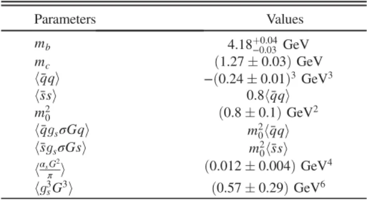
The obtained sum rules depend on the quark, gluon, and mixed condensates, the numerical values of which are collected in TableI. This table also contains the masses of the b and c quarks, which appear in the sum rules as input parameters.

Besides, Eqs. (12) and (13) depend on the auxiliary parameters M2 _{and s}

0, which should satisfy the standard

constraints of the sum rule computations. Our analysis proves that the working windows

TABLE I. The parameters utilized in our numerical computations. Parameters Values mb 4.18þ0.04_−0.03 GeV mc ð1.27 # 0.03Þ GeV h¯qqi −ð0.24 # 0.01Þ3 _GeV3 h¯ssi 0.8_h¯qqi m2 0 ð0.8 # 0.1Þ GeV2 h¯qgsσGqi m20h¯qqi h¯sgsσGsi m20h¯ssi hαsG2 π i ð0.012 # 0.004Þ GeV 4 hg3 sG3i ð0.57 # 0.29Þ GeV6

M2_{∈ ½9; 13( GeV}2_{; s}

0∈ ½115; 120( GeV2 ð16Þ

meet all of the restrictions imposed on M2_{and s}

0. Thus, the

maximum of the Borel parameter is determined from the minimum allowed value of the pole contribution (PC), which at M2_{¼ 13 GeV}2 _{is 16% of the full correlation}

function. Within the region M2_{∈ ½9; 13( GeV}2 _{the pole}

contribution varies from 59 to 16%. The lower limit of the Borel parameter is fixed by the convergence of the operator product expansion (OPE) for the correlation function. In the present work, we use the criterion

RðM2 Þ ¼ΠDimð8þ9þ10ÞðM 2_{; s} 0Þ ΠðM2_{; s} 0Þ < 0.05; _ð17Þ where ΠðM2_{; s}

0Þ is the Borel-transformed and subtracted

function ΠOPE_ðp2_{Þ, and ΠDimð8þ9þ10ÞðM}2_{; s}

0Þ is the

con-tribution from the last three terms in its expansion. At M2_¼

9 GeV2_{the ratio R is equal to Rð9 GeV}2

Þ ¼ 0.01, which ensures the excellent convergence of the sum rules. Moreover, at M2_{¼ 9 GeV}2 _{the perturbative contribution}

amounts to 74% of the full result, considerably exceeding the nonperturbative terms.

The quantities evaluated by means of the sum rules, in general, should not depend on the auxiliary parameters M2

and s0. But in calculations of the mass m and coupling f we

observe a residual dependence on M2_{and s}

0. Therefore, the

stability of the extracted parameters (i.e., m and f) is a necessary condition to fix the working windows for M2_and

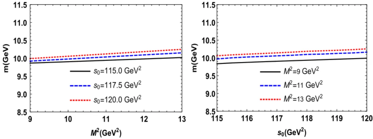
s0. In Figs.1and2we plot the dependence of the mass and

coupling of the tetraquark T−

bb;¯u ¯don the parameters M2and

s0. It is seen that m and f depend on M2 and s0, which

generates the main part of the theoretical errors inherent to the sum rule computations. For the mass m these ambi-guities are small, whereas for the coupling f they may be sizable. This behavior has a simple explanation: the sum rule for the mass of the tetraquark(12)is given as the ratio of integrals over the functions sρOPE_{ðsÞ and ρ}OPE_{ðsÞ, which}

considerably reduces effects due to the variation of M2_and

s0. The coupling f depends on the integral over the spectral

density ρOPE

ðsÞ itself, and therefore undergoes relatively sizable changes. In the case under discussion, theoretical errors for m and f stemming from the uncertainties of M2

and s0and other input parameters are #2.6 and #20% of

the corresponding central values, respectively.

Our analysis for the mass and coupling of the tetraquark T−

bb; ¯d ¯upredicts

m ¼ ð10035 # 260Þ MeV;

f ¼ ð1.38 # 0.27Þ × 10−2 _GeV4_{: ð18Þ}

Similar studies of Z0

bc lead to the following results:

mZ¼ ð6660 # 150Þ MeV;

fZ¼ ð0.51 # 0.16Þ × 10−2 GeV4; ð19Þ

which have been obtained using the working regions M2_{∈ ½5.5; 6.5( GeV}2_{; s}

0∈ ½53; 55( GeV2: ð20Þ

It is worth noting that in the calculations of mZand fZthe

PC changes by 55 to 21%. The contribution of the last three terms to the corresponding correlation function at the point M2

¼ 5.5 GeV2_{amounts to 1.9% of the total result, which}

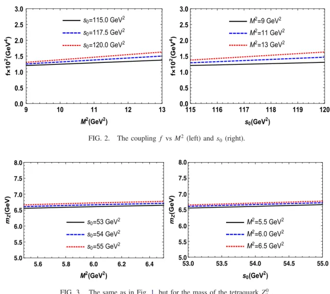
guarantees the convergence of the sum rules. In Figs. 3

and4we depict the mass and coupling of the tetraquark Z0 bc

as a function of M2 _{and s}

0 to demonstrate their residual

dependence on these parameters. It is evident that, as in the case of the T−

bb;¯d ¯ustate, the mass mZis less sensitive to

variations of M2 _{and s}

0 than the coupling fZ. But, the

relevant theoretical errors stay within the allowed limits inherent to sum rule computations, which may equal up to #30% of the predictions.

As it has been noted above, the mass of the state T− bb;¯u ¯d

was evaluated using different approaches in Refs.[18,19]

FIG. 1. The mass of the tetraquark T−

and [26]. The investigations in the first two papers were carried out in the framework of the sum rules method, and therefore we first compare our result for m with those predictions. Our result for m is smaller than the prediction m ¼ 10.2 # 0.3 GeV made in Ref. [18]: there is an over-lapping region between these two results, but the central

values differ from each other. This discrepancy is presumably connected with the accuracy of the analysis performed there (up to dimension-eight condensates), and with the choice of the working intervals for the parameters M2_{and s}

0.

Thus, in Ref. [18] the explored range for the continuum threshold was 11.3≤ ffiffiffiffiffip ≤ 11.7 GeV, whereas the Borels0 FIG. 2. The coupling f vs M2 _{(left) and s}

0 (right).

FIG. 3. The same as in Fig. 1, but for the mass of the tetraquark Z0 bc.

parameter varied within the limits M2_{∈ ½7.5; 9.6( GeV}2_or

M2_{∈ ½7.5; 11.2( GeV}2_{. Because} ffiffiffiffiffi_s 0

p determines the mass of the first excited tetraquark T−

bb;¯u ¯dthe corresponding mass

gap amounts to _{Δm ¼ 1.30 # 0.36 GeV, which is larger} than the typical tetraquark valueΔmT∼ 0.5–0.7 GeV. In our

case, this mass gap is _{Δm ¼ 0.79 # 0.17 GeV and} over-shootsΔmT as well. But one should take into account that

the estimate ΔmT ∼ 0.6 GeV was made for tetraquarks

lying near or above the corresponding two-meson thresholds, and therefore this fact may be connected with the stable nature of T−

bb; ¯u ¯d.

The sum rules analysis of the state T−

bb;¯u ¯dwas performed

in Ref.[19]by employing various interpolating currents ηi.

In computations the continuum threshold s0¼ 115 GeV2

and different regions for the Borel parameter were used, with M2_{¼ ½6.5; 8.6( GeV}2 _{and M}2_{¼ ½7.0; 9.2( GeV}2

being two extreme choices for M2_{. The mass of the}

axial-vector tetraquark T−

bb;¯u ¯d in Ref. [19] was found to

be m ¼ 10.2 # 0.3 GeV. Here we also underline a differ-ence between the Borel windows in Ref.[19]and those in the present work as a possible source of this deviation.

The recent model analysis of Ref. [26] predicted m ¼ 10389 # 12 MeV, which is considerably larger than the present result. Nevertheless, all calculations confirm that the tetraquark T−

bb;¯u ¯d is stable against the strong and

electromagnetic decays and can only dissociate weakly. The tetraquarks Zbc ¼ ½bc(½¯q ¯q( (q ¼ u, d) were

inves-tigated in Ref.[41]by employing the QCD sum rule method and various interpolating currents. The masses of the charged scalar tetraquarks Z−

bc; ¯u ¯u¼ ½bc(½¯u ¯u( and Zþbc;¯d ¯d¼ ½bc(½¯d ¯d(

found there were m ¼ 7.14 # 0.10 GeV. This prediction is considerably higher than our present result for mZ. But one

should take into account that the scalar tetraquark Z0 bc;¯u ¯d¼

½bc(½¯u ¯d( has different quark content: it is a neutral particle and contains [like the resonance Xð5568Þ] four quarks of different flavors. Therefore, a discrepancy between the predictions for Zbc and Z0bc may be explained not only by

the accuracy of the corresponding sum rule analysis and different working regions for the parameters M2_{and s}

0, but

also by the aforementioned reasons. In Ref.[47]the masses of the ground-state tetraquarks QQ0_{u ¯d in the context of¯}

the Bethe-Salpeter method. In the case of the state Z0 bc, using

one of parameter sets the authors found that its mass is m ¼ 6.93 GeV: this estimate is closer to our prediction.

III. SEMILEPTONIC DECAY T_{bb; ¯u ¯d}− → Z0bcl ¯νl

The semileptonic decay of the tetraquark T−

bb;¯u ¯d to the

final state Z0

bcl¯νlruns through the chain of transitions b →

W−_{c and W}− _{→ l¯ν. As is seen from results obtained in the}

previous section, the difference between the initial and final tetraquark masses is large enough to make all of the decays (l ¼ e, μ, and τ) kinematically allowed processes.

At the tree level the transition b → c can be described using the effective Hamiltonian

Heff_¼GF

ffiffiffi 2

p Vbccγ¯ μð1 − γ5Þb¯lγμð1 − γ5Þνl; ð21Þ

where GF is the Fermi coupling constant and Vbc is the

corresponding element of the Cabibbo-Kobayashi-Maskawa (CKM) matrix. After sandwiching the Heff _{between the}

initial and final tetraquarks and factoring out the lepton fields, we get the matrix element of the current

Jtr

μ ¼ ¯cγμð1 − γ5Þb ð22Þ

in terms of the form factors Giðq2Þ that parametrize the

long-distance dynamics of the weak transition[48], hZðp0_ÞjJtr

μjTðp; ϵÞi ¼ ˜G0ðq2Þϵμþ ˜G1ðq2Þðϵp0ÞPμ

þ ˜G2ðq2Þðϵp0Þqμþ i ˜G3ðq2Þεμναβϵνpαp0β: ð23Þ

The scaled functions ˜Giðq2Þ above are connected with

the dimensionless form factors Giðq2Þ by the following

equalities: ˜ G0ðq2Þ ¼ ˜mG0ðq2Þ; G˜jðq2Þ ¼ Gjðq2Þ ˜ m ; j ¼ 1; 2; 3: ð24Þ In Eqs. (23) and (24) _{m ¼ m þ m}˜ Z, p and ϵ are the

momentum and polarization vector of the tetraquark T−

bb; ¯u ¯d, p0 is the momentum of the state Z0bc, Pμ¼

p0

μþ pμ, and qμ¼ pμ− p0μ is the momentum transferred

to the leptons. It is clear that q2_{changes within the limits}

m2

l ≤ q2≤ ðm − mZÞ2, where mlis the mass of the lepton l.

The form factors Giðq2Þ are quantities that should be

extracted from the sum rules which, in turn, are obtainable from an analysis of the three-point correlation function

Πμνðp; p0Þ ¼ i2 Z d4_xd4_yeiðp0_y−pxÞ × h0jT fJZ_ðyÞJtr μð0ÞJ†νðxÞgj0i; ð25Þ where J_{νðxÞ and J}Z

ðyÞ are the interpolating currents to the T−

bb; ¯u ¯dand Z0bc states, respectively.

To derive sum rules for the weak form factors we express the correlation functionΠμνðp; p0Þ in terms of the masses

and couplings of the involved particles, and thus determine the physical or phenomenological side of the sum rule ΠPhysμν ðp; p0Þ. We also calculate Πμνðp; p0Þ using the

inter-polating currents and quark propagators, which leads to its expression in terms of the quark, gluon, and mixed vacuum condensates. By matching the obtained results and employ-ing the assumption on the quark-hadron duality, it is possible

to extract sum rules and evaluate the physical parameters of interest.

The functionΠPhysμν ðp; p0Þ can be easily written down in

the form ΠPhysμν ðp; p0Þ ¼h0jJ Z jZðp0_ÞihZðp0_ÞjJtr μjTðp; ϵÞi ðp2_{− m}2_Þðp02_{− m}2 ZÞ × hTðp; ϵÞjJ†νj0i þ ) ) ) ; ð26Þ

where we only take into account contributions arising from the ground-state particles, and effects of the excited and continuum states are denoted by dots.

The phenomenological side of the sum rules can be further simplified by rewriting the relevant matrix elements in terms of the tetraquark parameters, and employing for hZðp0_ÞjJtr

μjTðp; ϵÞi its expression through

the weak transition form factors Giðq2Þ. The matrix

elements of the tetraquarks T−

bb;¯u ¯d and Z0bc are known

and given by Eqs.(6) and (14), respectively. The matrix

element hZðp0_ÞjJtr

μjTðp; ϵÞi is modeled by means of the

four transition form factors Giðq2Þ which can be used

calculate all three semileptonic decays.

Substituting the relevant matrix elements into Eq.(26), forΠPhysμν ðp; p0; q2Þ we finally get

ΠPhysμν ðp; p0; q2Þ ¼ fmfZmZ ðp2_{− m}2_Þðp02_{− m}2 ZÞ × $ ˜ G0ðq2Þ ! −gμνþ pμpν m2 " þ ½ ˜G1ðq2ÞPμþ ˜G2ðq2Þqμ( × ! −p0_νþm2þ m2Z− q2 2m2 pν " − i ˜G3ðq2Þεμναβpαp0β % þ ) ) ) ð27Þ The functionΠOPE

μν ðp; p0Þ constitutes the second side of

the sum rules and has the following form:

ΠOPE μν ðp; p0Þ ¼ Z d4_xd4_yeiðp0_y−pxÞ fTr½γ5˜Sb 0b d ðx − yÞγ5Sa 0_a

u ðx − yÞ(ðTr½γμ˜Saab0ðy − xÞγ5SbicðyÞγνð1 − γ5Þ

×Sib0 b ð−xÞ( þ Tr½γμ˜Sia 0 b ð−xÞð1 − γ5Þγν˜Sbic ðyÞγ5Sab 0 b ðy − xÞ(Þ − Tr½γ5˜Sb 0_a d ðx − yÞγ5Sa 0_b u ðx − yÞ( × ðTr½γμ˜Saa 0 b ðy − xÞγ5Sbic ðyÞγνð1 − γ5ÞSib 0 b ð−xÞ( þ Tr½γμ˜Sia 0 b ð−xÞð1 − γ5Þγν˜SbicðyÞγ5Sab 0 b ðy − xÞ(Þg: ð28Þ

To extract the sum rules for the form factors Giðq2Þ, we

equate invariant amplitudes corresponding to the same Lorentz structures in ΠPhysμν ðp; p0; q2Þ and ΠOPEμν ðp; p0Þ,

perform a double Borel transformation over the variables p02 _{and p}2_{to suppress contributions of the higher excited}

and continuum states, and perform continuum subtraction. For example, to extract the sum rule for ˜G0ðq2Þ we use the

structure gμν, whereas for ˜G3ðq2Þ we employ the term

∼εμναβpαp0β. It is convenient to present the obtained sum

rules in a single formula through the functions ˜Giðq2Þ,

˜ GiðM2; s0; q2Þ ¼ 1 fmfZmZ Z _s 0 4m2 b ds Z _s0 0 ðmbþmcÞ2 ds0 × ρiðs; s0; q2Þeðm 2_−sÞ=M2 1eðm 2 Z−s0Þ=M22; ð29Þ

bearing in mind that they are connected to the dimension-less form factors Giðq2Þ by Eq.(24). Here M2¼ ðM21; M22Þ

are the Borel parameters, and s0¼ ðs0; s00Þ are the

tinuum threshold parameters that separate the main con-tribution to the sum rules from the continuum effects. The sum rules(29)are written down using the spectral densities ρiðs; s0; q2Þ which are proportional to the imaginary parts

of the corresponding invariant amplitudes in ΠOPE μν ðp; p0Þ.

They contain the perturbative and nonperturbative contri-butions, and are calculated with dimension-six accuracy.

For numerical computations of the weak form factors GiðM2; s0; q2Þ one needs to fix various parameters. Values

some of these parameters are collected in TableI, while the masses and couplings of the tetraquarks T−

bb;¯u ¯d and Z0bc

were evaluated in the previous section. In the present computations, we impose the same constraints on the auxiliary parameters M2_{and s}

0as in the mass calculations.

To obtain the width of the decay T−

bb;¯u ¯d→ Z0bcl¯νlone has

to integrate the differential decay rate dΓ=dq2_{(for details,}

see the Appendix) within allowed kinematical limits m2 l ≤

q2_{≤ ðm − m}

ZÞ2. It is clear that for light leptons l ¼ e; μ

the lower limit of the integral is considerably smaller than 1 GeV2_{, but the perturbative calculations lead to reliable}

predictions for momentum transfers q2_{> 1 GeV}2_{. Therefore,}

we use the usual prescription and replace the weak form factors in the whole integration region by fit functions Fiðq2Þ,

which for perturbatively allowed values of q2 _{coincide with}

Giðq2Þ.

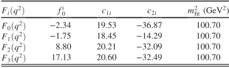
There are various analytical expressions for the fit functions. In the present paper we utilize

Fiðq2Þ ¼ fi0exp & c1i q2 m2 fitþ c2i ! q2 m2 fit "₂' ; ð30Þ

where fi

0, c1i, c2i, and m2fitare fitting parameters. The values

of these parameters are presented in TableII. Besides that, for the numerical calculations we need the Fermi coupling constant GFand CKM matrix element jVbcj, for which we use

GF ¼ 1.16637 × 10−5 GeV−2;

jVbcj ¼ ð41.2 # 1.01Þ × 10−3: ð31Þ

As a result, for the decay width of the processes T− bb;¯u ¯d→

Z0

bcl¯νl(l ¼ e; μ, and τ) we find

ΓðT−

bb;¯u ¯d→ Z0bce¯νeÞ ¼ ð2.65 # 0.78Þ × 10−8 MeV;

ΓðT−

bb; ¯u ¯d→ Z0bcμ¯νμÞ ¼ ð2.64 # 0.78Þ × 10−8 MeV;

ΓðT−

bb;¯u ¯d→ Z0bcτ¯ντÞ ¼ ð1.88 # 0.55Þ × 10−8 MeV; ð32Þ

which are the main results of the present work.

The partial decay widths from Eq.(32) can be used to estimate the full width and mean lifetime of the tetraquark T−

bb; ¯u ¯d

Γ ¼ ð7.17 # 1.23Þ × 10−8 _MeV;

τ ¼ 9.18þ1.90

−1.34× 10−15 s: ð33Þ

These predictions can be employed to explore the double-heavy tetraquarks.

IV. ANALYSIS AND CONCLUSIONS The spectroscopic parameters of the tetraquarks T−

bb;¯u ¯d

and Z0

bc as well as the width of the semileptonic decay

T−

bb; ¯u ¯d→ Z0bcl¯νl provide very interesting information on

the properties of four-quark systems. Thus, the mass of the tetraquark T−

bb;¯u ¯d obtained in the present work confirms

once more that it is stable against strong and electromag-netic decays, and can transform only weakly to a tetraquark Z0

bc and a pair of leptons l¯νl. This conclusion is valid even

when taking into account uncertainties inherent to the sum rule computations. Our result for m is smaller than the predictions made in Refs.[18]and[26]using the QCD sum rule method and phenomenological model estimations, respectively. The semileptonic decays T−

bb;¯u ¯d→ Z0bcl¯νl,

where l ¼ e, μ and τ have allowed us to evaluate the width of T−

bb;¯u ¯d and its mean lifetime τ ¼ 9.18þ1.90−1.34 fs, which is

considerably shorter than the prediction of Ref.[26]. Another interesting result of this work is connected with the parameters of the scalar tetraquark Z0

bccomposed of the

heavy diquark bc and light antidiquark ¯u ¯d. In fact, the mass of this state mZ ¼ ð6660 # 150Þ MeV is

consider-ably below the threshold ≈7145 MeV for strong S-wave decays to conventional heavy B−_Dþ _{and B}0_D0 _mesons.

Because of its quark content, Z0

bc cannot decay to a pair of

heavy and light mesons as well. These features differ qualitatively from those of the open charm-bottom scalar tetraquarks Zq¼ ½cq(½¯b ¯q( and Zs¼ ½cs(½¯b ¯s(, which decay

strongly to Bcπ and Bcη mesons[44], and, in turn, cannot

decay to two heavy mesons. In other words, the four-quark system consisting of a heavy diquark and a light anti-diquark is more stable than one consisting of a heavy-light diquark and antidiquark. This is seen from a comparison of the masses of the tetraquark Z0

bc and the state Zq, for

which mZq ¼ ð6.97 # 0.19Þ GeV.

Theoretical information on the decay properties of the state T−

bb;¯u ¯dcan be further improved by including its other

weak decay channels in analyses. The investigation of the stable open charm-bottom tetraquarks Z0

bc with different

quantum numbers is also an interesting topic of exotic hadron physics: by clarifying these problems we can deepen our understanding of multiquark systems.

ACKNOWLEDGMENTS

S. S. A. is grateful to Prof. V. M. Braun for enlightening discussions. K. A., B. B., and H. S. thank the scientific and technological research council of Turkey (TUBITAK) for the partial financial support provided under Grant No. 115F183.

APPENDIX: THE DECAY RATE d_Γ=dq2

This appendix contains the explicit expression for the decay rate dΓ=dq2_{necessary to calculate the width of the}

semileptonic decay T−

bb; ¯u ¯d→ Z0bcl¯νl. Calculations lead to

the following result:

dΓ dq2¼ G2 FjVcbj2 3 · 28_π3_m3 !q2_{− m}2 l q2 " λðm2_{; m}2 Z; q2Þ &Xi¼3 i¼0 ˜ G2 iðq2ÞAiðq2Þ þ ˜G0ðq2Þ ˜G1ðq2ÞA01ðq2Þ þ ˜G0ðq2Þ ˜G2ðq2ÞA02ðq2Þ þ ˜G1ðq2Þ ˜G2ðq2ÞA12ðq2Þ ' : ðA1Þ

TABLE II. The parameters of the fit functions Fiðq2Þ.

Fiðq2Þ fi0 c1i c2i m2fit (GeV2)

F0ðq2Þ −2.34 19.53 −36.87 100.70

F1ðq2Þ −1.75 18.45 −14.29 100.70

F2ðq2Þ 8.80 20.21 −32.09 100.70

In Eq.(A1) the functions Aiðq2Þ and Aijðq2Þ are given by A0ðq2Þ ¼ 1 2m2_q4½q 4_ðm2_{− m}2 ZÞ2− 4q4m2m2l − m4lðm2− m2Zþ q2Þ2þ 2q6ð3m2− m2ZÞ þ q8(; A1ðq2Þ ¼ 1 2m2_q4½m 4 þ ðm2 Z− q2Þ2− 2m2ðm2Zþ q2Þ(fm4lðm2− m2ZÞ2þ q4ml4ðq2− 2m2− 2m2ZÞ −q4_½m4_{þ ðm}2 Z− q2Þ2− 2m2ðm2Zþ q2Þ(g; A2ðq2Þ ¼ m2 l 2m2ðq 2_{− m}2 lÞ½m4þ ðm2Z− q2Þ2− 2m2ðm2Zþ q2Þ(; A3ðq2Þ ¼ 1 2q2ðm 4 l − q4Þ½m4þ ðm2Z− q2Þ2− 2m2ðm2Zþ q2Þ(; A01ðq2Þ ¼ 1 m2_q4½q 4_ðm2 lþ m2Z− m2− q2Þ þ m4lðm2− m2ZÞ(½m4þ ðm2Z− q2Þ2− 2m2ðm2Zþ q2Þ(; A02ðq2Þ ¼ m2 lðm2l − q2Þ m2_q2 ½m 4 þ ðm2 Z− q2Þ2− 2m2ðm2Zþ q2Þ(; A12ðq2Þ ¼ m2 lðq2− m2lÞðm2− m2ZÞ m2_q2 ½m 4_{þ ðm}2 Z− q2Þ2− 2m2ðm2Zþ q2Þ(; ðA2Þ and λðm2_{; m}2 Z; q2Þ ¼ ½m4þ m4Zþ q4− 2ðm2m2Zþ m2q2þ m2Zq2Þ(1=2:

[1] R. L. Jaffe,Phys. Rev. D 15, 267 (1977). [2] R. L. Jaffe,Phys. Rev. D 15, 281 (1977).

[3] J. D. Weinstein and N. Isgur, Phys. Rev. Lett. 48, 659 (1982).

[4] J. P. Ader, J. M. Richard, and P. Taxil,Phys. Rev. D 25, 2370 (1982).

[5] H. X. Chen, W. Chen, X. Liu, and S. L. Zhu,Phys. Rep. 639, 1 (2016).

[6] A. Esposito, A. Pilloni, and A. D. Polosa,Phys. Rep. 668, 1 (2017).

[7] A. Ali, J. S. Lange, and S. Stone,Prog. Part. Nucl. Phys. 97, 123 (2017).

[8] S. L. Olsen, T. Skwarnicki, and D. Zieminska,Rev. Mod. Phys. 90, 015003 (2018).

[9] H. J. Lipkin, Phys. Lett. B 172, 242 (1986).

[10] S. Zouzou, B. Silvestre-Brac, C. Gignoux, and J. M. Richard,Z. Phys. C 30, 457 (1986).

[11] J. Carlson, L. Heller, and J. A. Tjon,Phys. Rev. D 37, 744 (1988).

[12] A. V. Manohar and M. B. Wise, Nucl. Phys. B399, 17 (1993).

[13] S. Pepin, F. Stancu, M. Genovese, and J. M. Richard,Phys. Lett. B 393, 119 (1997).

[14] D. Janc and M. Rosina, Few Body Syst. 35, 175 (2004).

[15] Y. Cui, X. L. Chen, W. Z. Deng, and S. L. Zhu, High Energy Phys. Nucl. Phys. 31, 7 (2007).

[16] J. Vijande, A. Valcarce, and K. Tsushima,Phys. Rev. D 74, 054018 (2006).

[17] D. Ebert, R. N. Faustov, V. O. Galkin, and W. Lucha,Phys. Rev. D 76, 114015 (2007).

[18] F. S. Navarra, M. Nielsen, and S. H. Lee,Phys. Lett. B 649, 166 (2007).

[19] M. L. Du, W. Chen, X. L. Chen, and S. L. Zhu,Phys. Rev. D 87, 014003 (2013).

[20] J. Schaffner-Bielich and A. P. Vischer, Phys. Rev. D 57, 4142 (1998).

[21] A. Del Fabbro, D. Janc, M. Rosina, and D. Treleani,Phys. Rev. D 71, 014008 (2005).

[22] S. H. Lee, S. Yasui, W. Liu, and C. M. Ko,Eur. Phys. J. C 54, 259 (2008).

[23] T. Hyodo, Y. R. Liu, M. Oka, K. Sudoh, and S. Yasui,Phys. Lett. B 721, 56 (2013).

[24] A. Esposito, M. Papinutto, A. Pilloni, A. D. Polosa, and N. Tantalo,Phys. Rev. D 88, 054029 (2013).

[25] R. Aaij et al. (LHCb Collaboration),Phys. Rev. Lett. 119, 112001 (2017).

[26] M. Karliner and J. L. Rosner,Phys. Rev. Lett. 119, 202001 (2017).

[27] S. Q. Luo, K. Chen, X. Liu, Y. R. Liu, and S. L. Zhu,

Eur. Phys. J. C 77, 709 (2017).

[28] E. J. Eichten and C. Quigg, Phys. Rev. Lett. 119, 202002 (2017).

[29] Z. G. Wang and Z. H. Yan,Eur. Phys. J. C 78, 19 (2018). [30] A. Ali, A. Y. Parkhomenko, Q. Qin, and W. Wang,Phys.

Lett. B 782, 412 (2018).

[31] A. Ali, Q. Qin, and W. Wang,Phys. Lett. B 785, 605 (2018). [32] E. Eichten and Z. Liu,arXiv:1709.09605.

[33] C. Hughes, E. Eichten, and C. T. H. Davies,Phys. Rev. D 97, 054505 (2018).

[34] A. Esposito and A. D. Polosa, Eur. Phys. J. C 78, 782 (2018).

[35] S. S. Agaev, K. Azizi, B. Barsbay, and H. Sundu, Nucl. Phys. B939, 130 (2019).

[36] H. Sundu, B. Barsbay, S. S. Agaev, and K. Azizi,Eur. Phys. J. A 54, 124 (2018).

[37] Y. Xing and R. Zhu,Phys. Rev. D 98, 053005 (2018). [38] B. Silvestre-Brac and C. Semay,Z. Phys. C 59, 457 (1993).

[39] Z. F. Sun, X. Liu, M. Nielsen, and S. L. Zhu,Phys. Rev. D 85, 094008 (2012).

[40] R. M. Albuquerque, X. Liu, and M. Nielsen,Phys. Lett. B 718, 492 (2012).

[41] W. Chen, T. G. Steele, and S. L. Zhu, Phys. Rev. D 89, 054037 (2014).

[42] J. R. Zhang and M. Q. Huang,Phys. Rev. D 80, 056004 (2009).

[43] J. R. Zhang and M. Q. Huang,Commun. Theor. Phys. 54, 1075 (2010).

[44] S. S. Agaev, K. Azizi, and H. Sundu, Phys. Rev. D 95, 034008 (2017).

[45] S. S. Agaev, K. Azizi, and H. Sundu,Eur. Phys. J. C 77, 321 (2017).

[46] V. M. Abazov et al. (D0 Collaboration),Phys. Rev. Lett. 117, 022003 (2016).

[47] G.-Q. Feng, X.-H. Guo, and B.-S. Zou,arXiv:1309.7813. [48] P. Ball, V. M. Braun, and H. G. Dosch, Phys. Rev. D 44,