ON THE STABILITY LOSS OF THE CIRCULAR CYLINDER MADE FROM VISCOELASTIC COMPOSITE MATERIAL

1

Research Article / Araştırma Makalesi

ON THE STABILITY LOSS OF THE CIRCULAR CYLINDER MADE FROM

VISCOELASTIC COMPOSITE MATERIAL

Şerife KARAKAYA

*

İstanbul Aydin University, Faculty of Arts and Science, Department of Statistics, Küçükçekmece-İSTANBUL Received/Geliş: 20.01.2011 Revised/Düzeltme: 19.04.2011 Accepted/Kabul: 27.04.2011

ABSTRACT

The 3D approach was employed for investigations of the stability loss of the cylinder with circular cross section fabricated from the viscoelastic composite materials. This approach is based on the investigations of the development of the initial infinitesimal imperfections of the cylinder within the scope of the 3D geometrically nonlinear field equations of the theory of the viscoelasticity for anisotropic bodies. The numerical results on the critical forces and critical time are presented and discussed.

Keywords: Stability loss, cylinder made from viscoelastic composite material, boundary form perturbation method.

VİSKOELASTİK KOMPOZİT MALZEMEDEN YAPILMIŞ DAİRESEL SİLİNDİRİN STABİLİTESİNİN KAYBI HAKKINDA

ÖZET

Viskolelastik kompozit malzemeden yapılmış dairesel silindirin 3 boyutlu stabilite kaybının incelenmesi için yaklaşım önerilmektedir. Bu yaklaşım, anizotrop cisimler için, viskoelastisite teorisinin, 3 boyuttlu, geometrik olarak doğrusal olmayan, alan denklemleri çerçevesinde silindire ait başlangıçtaki sonsuz küçük sapmanın gelişiminin araştırılmasına dayanmaktadır. Kritik kuvvet ve kritik zamana ait sayısal sonuçlar bulunmuş ve tartışılmıştır.

Anahtar Sözcükler: Stabilite kaybı, viskoelastik kompozit malzemeden yapılmış silindir, sınır formu pertürbasyon yöntemi.

1. INTRODUCTION

In the paper [1,2] and others, the 3D approach was proposed for investigations of the stability loss of the elements of constructions fabricated from the viscoelastic composite materials. This approach is based on the investigations of the development of the initial infinitesimal imperfections of these elements of constructions within the scope of the 3D geometrically nonlinear field equations of the theory of the viscoelasticity for anisotropic bodies. The review of the investigations carried out by utilizing the mentioned approach is given in a paper [3]. It follows from this review that, up the now the corresponding problem for cylinders do not studied.

* _{serifekarakaya@aydin.edu.tr, tel: (212) 411 61 59}

Journal of Engineering and Natural Sciences

Mühendislik ve Fen Bilimleri Dergisi

Sigma 31,

1-19,

2012

2

In the present paper the first attempt is made in this field and the stability loss of the circular cylinder fabricated from viscoelastic composite material is studied.

Throughout the investigations, repeated indices are summed over their ranges.

2. FORMULATION OF THE PROBLEM

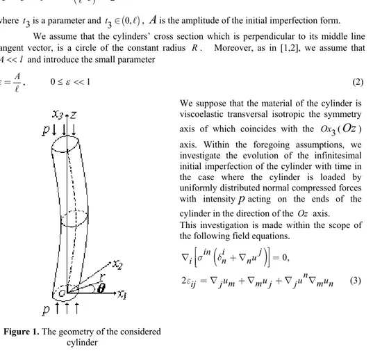
We consider a cylinder which has an initial imperfection in the natural state and determine the position of the points of this cylinder with the Lagrange coordinates in the cylindrical Or zq and

the Cartesian system of coordinates Ox x x system of coordinates (Fig. 1). The noted initial _{1 2 3}

imperfection is given through the following equation of the middle line of the cylinder 3 3

x =t

;

x₁=Asin_çèççæp_t₃ö÷÷_÷ø

;

x₂ (1) 0 where 3t is a parameter and t Î₃

( )

0, ,

A

is the amplitude of the initial imperfection form.

We assume that the cylinders’ cross section which is perpendicular to its middle line tangent vector, is a circle of the constant radius R . Moreover, as in [1,2], we assume that

l

A and introduce the small parameter

A e =

, 01 (2)

Figure 1. The geometry of the considered cylinder

We suppose that the material of the cylinder is viscoelastic transversal isotropic the symmetry axis of which coincides with the Ox (₃

Oz

) axis. Within the foregoing assumptions, we investigate the evolution of the infinitesimal initial imperfection of the cylinder with time in the case where the cylinder is loaded by uniformly distributed normal compressed forces with intensity

p

acting on the ends of the cylinder in the direction of the Oz axis.

This investigation is made within the scope of the following field equations.

(

j

)

0, in i _u n n i s d 

é

_ê

_ë

+ 

ù

_ú

_û

= 2e = _{ij j}u_m+ _mu_j+ _jun_{m n}u (3)

The constitutive relations for the cylinder material in the cylindrical system of coordinates are given as follows:

3

; ; 11 12 13 12 11 13 A A A _zz A A A _zz rr rr rr s = *e + *e_qq+ *e s_qq= *e + *e_qq+ *e

(

)

; ; 13 13 33 11 22 A A A A A zz rr zz _{r r} s = *e + *e_qq+ *e s _q= * - * e _q 2G ; 2G , rz rz _{z z} s = *e s_q = *e_q (4) where A and _ij G are following operators

 

 









 

0 1 0 0 1 A A t A_{ij ij} t _ij t t d G G t G         _{  }       _  _{ }   _        _ _       (5) Here, _{Aij and 00} G are the instantaneous values of elastic constants, A_ij1

( )

t and G t

( )

are the given functions which determine the hereditary properties of the cylinder material. Assume that on the lateral surface S of the cylinder the following conditions are satisfied

(

j j

)

0

in _{u n}

n n _{S j}

s d +  = (6) In the natural state, the upper and lower ends of the cylinder are on the inclined planes with unit normal vectors

0 ₁ 2 2 k i n ep e p -= +   

(for lower end plane)

2 2 1 k i n_l ep e p -= +   

(for upper end plane) (7) Denote the upper (lower) end cross section of the cylinder through S S_

( )

₀ and the conditions for the forces on these end cross sections can be written as follows:

(

)

(

)

3 _, 3 0 0 j j j j n _{u n p} n _{u n p} n n _{S j} n n _{S lj} s d +  = s d +  = - (8) The end conditions for the displacements will be discussed below.

Note that in (3), (4), (6), (7) and (8) the following notation is used: i shows the covariant derivatives with respect to the i-th cylindrical coordinate, in is a contravariant component of the stress tensor, ij is a covariant component of the Green’s strain tensor,

( )

n

u u_n is a covariant (contravariant) component of the displacement vector,



rr zz



zz

rr     

 , ,..., , , ,..., is a physical component of the stress (strain) tensor in the cylindrical system of coordinates Or zq ; _ni _{is the Kronecker symbol; n j is a covariant} component of the unit normal vector of the lateral surface of the cylinder; 0n j

( )

n j is a

covariant component of the unit normal vector of the end inclined plane at t =₃ 0

(

t = ₃

)

. Moreover, below we will use the notation ur , uq and uz for denoting the physical components

4

of the displacement vector. It is known that the mentioned physical components are determined according to the expressions s_{( )ij} =sijH H_{i j},

(

)

1 ( )ij ij H Hi j

e =e - , u_{( )i} =u Hi _i=u H_i

( )

_i -1

, where

 

ij rr,, , , ,zz r rz z , ( )i r, , z_{. Here Hi are Lamé’s coefficients and} H₁1.0, 2

H  , r H₃1.0 for the cylindrical system of coordinates. Thus, with this the formulation of the considered problem has been exhausted and it follows from this formulation that the evolution of the infinitesimal initial imperfection of the cylinder with time for the fixed value of the initial compressed force p (for the case where the material of the cylinder is viscoelastic) or with initial compressed force p (for the case where the material of the cylinder is pure elastic) will be investigated within the framework of the field equations (3), (4), (5) and boundary condition (6) and (8)

.

3. METHOD OF SOLUTION

Now we consider the method of solution of the problem formulated in the previous section. Note that the method employed below can be briefly summarized as follows. By employing the boundary-form perturbation techniques the considered boundary value problem for the non-linear integro-differential equations (3) – (5) is reduced to the series boundary-value problems for the corresponding system of the linear integro-differential equations. Owing to both the expressions of the operators (5) and the convolution theorem, by the use of the Laplace transform with respect to time these series problems are reduced to the corresponding series boundary value problems for the linear system of differential equations in the Laplace transform parameter space. For each fixed value of this parameter the linear problems are solved by employing variable-separation method and finally, applying the Schapery [4] inverse transformation method we determine the sought values. It should be noted that for the case where the material of the cylinder is pure elastic, the operators (5) are replaced by mechanical constants and therefore instead of the integro-differential equations we obtain differential equations and the corresponding problems for these equations are also investigated in the framework of the above procedure but without employing the Laplace transform.

Since, according to the procedure summarized above and the problem statement, first we derive the equation for the lateral surface S of the cylinder. According to the condition of the cylinder’s cross section we can conclude that the coordinates of this surface must simultaneously satisfy the following equations.

 





'( )_{3 10 3} f t x f t    x₃₀  , t₃ 0





2 2 20 30 3 x  x t 



x₁₀f t

 

₃



2R2, (9) where f t

 

₃  sin



t₃  ,



f t'

 

₃ cos



t_{3  ; 10}



_{x , 20}x _{, 30}x are coordinates of the surface S . Note that the first equation in (9) is an equation of the plane perpendicular to the vector which is the tangent vector to the middle line of the fiber at the point that corresponds to the fixed value of the parameter 3t ; but the second equation in (9) is an equation of the circle which is counter to the cross section of the cylinder which rises on the foregoing plane.

Using the relations x₁₀rcos, sinx₂₀r  we obtain the following equation for the surface S in the cylindrical system of coordinates Or z :

5

( , , )₃

r r  t  , ( , , )z t ₃ z₀₁ t₃ (10) The explicit expressions of the functions ( , , )r t₃ , z₀₁( , , ) t₃ can also be attained from equation (9); in order not to take up too much space here, we will not present these expressions.

Using the assumption (2) and supposing that the conditions



f t'

 

₃



2 , after some 1 mathematical manipulations, we obtain the following equations.

 

, 3 0 1 k r R a _k t k        , 3 1 0

 

,3 k z t b _k t k        ,

 

1 _{0 0 3}, 1 k n_r c _k t k        , 1 0

 

, 3 k n d _k t k     _ , nz _{k 1}kg0k

 

, 3t     . (11) where nr , n, nz are physical components of the unit normal vector to the surface S . The explicit expressions of the functions ( , , )r t₃ , ( , , )z₀₁ t₃ _{, nr , n nz ,} a_ok

 

_{, 3}t ,

 

, 3 0

b _k  t , c_0k

 

_{, 3}t , d_0k

 

_{, 3}t and g_0k

 

_{, 3}t can also be attained from equation (9); in order not to take up too much space here, we will not present these expressions.

We write the equation of the planes on which lays lower and upper inclined ends of the cylinder

3 1

x = -epx _{(for the lower end) 3}x =epx₁+  (for the upper end) (12) According to Eq. (7), we can also present the expression of the components of the normal vectors to these ends as follows

(

)

1 2 4 1 ( ) ( ) 01 1 ₂ n =n_ = -ep_çèççæ - ep +O ep _÷÷_øö÷ , ₀₃ 1 1( )2

(

( )4

)

2 n = - -æçç_çè ep +O ep ö÷÷_÷ø,

(

)

1 _{2 4} 1 ( ) ( ) 3 ₂ n_ = -çæ_çèç ep +O ep ÷_÷ö÷_ø. (13) According to the procedures of the boundary perturbation technique, as in the works [5,6] and in many others, we attempt to solve the considered problem by employing the boundary form perturbation method. For this purpose the unknowns are presented in series form in  (2).



 ij; _{ij i}; ;u ui







( ) ; ( ) ( ) ( ); ;



0 q q ij q _uq _uq i ij i q       . (14) Substituting Eq. (15) into Eq. (3), we obtain set equations for each approximation (14). Using Eq. (11) we expand the values of each approximation (14) in series form in the vicinity of the point



r₀R z_{0 0}; t₃



. Substituting these last expressions in the boundary conditions in (6) and using the expressions of nr , n_ and nz given in (11), after some mathematical transformations we obtain boundary conditions which are satisfied at



rR z t;  ₃



for each approximation in Eq.(14). It is evident that for the zeroth approximation, Eq.(3) is valid and condition (6) is replaced by the same one satisfied at point



rR z t;  ₃



. We assume that

(0) ₁

u n

6

Kronecker symbols. According to this assumption, for the zeroth approximation, we obtain the following system of equations:

(0)ij ₀ i

  , 2_ij(0) _{j i}u(0) _{i j}u(0), (15) and boundary conditions

 

(0)_{ij r R} 0

 

 , (16) where ( )ij rr r rz, , , ( ) i r, , z.

Moreover, we obtain the following end conditions for zeroth approximation from (7), (8), (8) and (13).

(0)_{( , ,0)r} (0)_{( , , )r p}

zz zz

       , (17) Note that the mathematical procedure, according to which the end condition (17) is obtained, will be given below.

Taking the last assumption into account, for the subsequent approximations we obtain the following system of equations.





1 ( ) (0) ( ) ( ) ( ) 1 q q ij in _u q j q m in _u m j n n i   _m i   _    _   _       _ , 1 ( ) ( ) ( ) ( ) , ( ) 1 2 q q q q q m n m ij j i i j j i k m u u u u         



  . (18) The underlined terms in Eq. (18) are equal to zero for the first approximation. By direct verification it is proven that the left side of Eq. (18) coincide with the corresponding equations of the Three-Dimensional Linearized Theory of Stability (TDLTS) [7]. Dui to linearity the constitutive relations (4) are satisfied by each approximation separately, i.e.

( ) ( ) ( ) ( )_; ( ) ( ) ( ) ( )_; 11 12 13 12 11 13 q _A q _A q _A q q _A q _A q _A q zz zz rr rr rr s = *e + *e_qq + *e s_qq = *e + *e_qq + *e

(

)

( ) ( ) ( ) ( )_; ( ) ( )_; 13 13 33 11 22 q _A q _A q _A q q _{A A} q zz rr zz _{r r} s = *e + *e_qq + * e s _q = * - * e_q ( )q _2G ( )q _; ( )q _2G ( )q _, rz rz _{z z} s = *e s_q = *e_q (19) Now we write the boundary conditions given on the lateral surface of the cylinder for the first approximation by the physical components of the stress tensor.

(0) (0) ( ) ( ) (1) 1 1 ( )ir f _rir _zir           (0) (0) (0) _0, ( ) ( ) z ( ) r ir i i z    _{ }    (20) where ( )i r, , z. In Eq. (20) replacing ( )i with ,r and z we obtain the explicit form of the corresponding contact conditions in the considered approximation. Moreover, in Eq. (20) the following notation is used.

'( )cos( )₃ f t z     , ( )cos( )f₁ f t₃  ,₁ Rf t'( )cos( )₃  , ( )₃ ''( ) cos( )₃ f t f t r _R  _  _    , ( ) 3 sin( ) f t R _    , '( )₃

 

3 3 df t f t dt  ,

7

 

2 3 ''( )_{3 2} 3 d f t f t dt  . (21) Consider the satisfaction of the end conditions (8). To simply the discussion we rewrite these conditions in the Cartesian system of coordinates Ox x x . _{1 2 3}

; 3 0 3 0 u_j u_j j _{n p} j _{n p} n n n _xn j n _xn j S S s ççç_çæ_çd +¶_¶ ö_÷÷÷_÷÷÷ = s ççæ_çççd +_¶¶ ÷÷÷ö_÷÷_÷ = -è ø è ø   (22) According to equation (12) and (13), we can write the following expressions from the conditions (22). ( , , , ) 1 1 1 2 1 ( , , , ) 3 0 3 1 2 1 01 0 u_{j u x x x t} j _{n x x x t n} n n n _xn j n _xn S ep s ç_çççæd +¶_¶ ö_÷÷÷_÷÷ =s -ep _çççæ_çd +¶ _¶ - ÷_÷÷÷ö÷ + ÷ ç è ø è ø ( , , , ) 3 3 1 2 1 ( , , , ) 3 1 2 1 03 u x x x t x x x t _n n p n _xn ep s -ep æçç_çd +¶ - ö÷÷_÷ = -÷÷ ç ¶ è ø ( , , , ) 1 1 1 2 1 ( , , , ) 3 3 1 2 1 1 u_j u x x x t j _{n x x x t n} n n n _xn j n _xn S ep s ç_èçæçççd +¶¶ ÷÷÷÷_ø÷÷ö =s +ep ççèçæçd +¶ ¶ + ÷ø÷ö÷÷÷ +      ( , , , ) 3 3 1 2 1 ( , , , ) 3 1 2 1 3 u x x x t x x x t _n n p n _xn ep s +ep æ_ççççd +¶ _¶ + ÷÷_÷÷ö÷ = è ø   _ (23) Using the expansions

( ,x x_{1 2}, x t₁, ) in    ( )( ,_{1 2}, ₁, ) (0)( ,_{1 2},0, ) 0 q q x xin x t in x x t q          

 

(0)( , ,0, )

 

2 (1)_{( , ,0, ) 1 2} 1 2 1 3 x x t in x x t x O in _x   _    _{ } _  _     ; ( ,_{1 2}, ₁, ) u_m x x x t x j      ( )_{( , , , )} (0)_{( , ,0, )} 1 2 1 1 2 0 q u_m x x x t u_m x x t q x x q _{j j}          _{ } 

 

 

(1)_{( , ,0, )} 2 (0)_{( , ,0, )} 2 1 2 1 2 1 3 u_m x x t u_m x x t x O x_j x x_j _ _    _{  } _  _     ; ( ,x x_{1 2}, x t₁, ) in    ( )( ,_{1 2}, ₁, ) (0)( ,_{1 2}, , ) 0 q q x xin x t in x x t q            

 

(0)( , , , )

 

2 (1)_{( , , , )} 1 2 1 2 1 3 x x t in x x t x O in _x   _    _{ } _ _       ;

8

( ,_{1 2}, ₁, ) u_m x x x t x j       ( )( ,_{1 2}, ₁, ) (0)( ,_{1 2}, , ) 0 q u_m x x x t u_m x x t q x x q _{j j}              

 

 

(1)_{( , , , )} 2 (0)_{( , , , )} 2 1 2 1 2 1 3 u_m x x t u_m x x t x O x_j x x_j _ _    _{  } _  _      

,

(24) we obtain the following expression for the end conditions (22).

(0) (0) (1) 2 (0) (0) 3 3 (0) 1 1 (0) 3 3 1 3 3 3 3 u u u u x k k _x k k _x k _{x x x} k k k k s d e ps d s p ì æ ö é æ ö æ ö ï _{÷ ÷ ÷} ï ç ¶ ÷ ê ç ¶ ÷ ç¶ ¶ ÷ ï ç ç ç ï- ç + ÷÷+ -ê ç + ÷÷- ç - ÷÷ -í _{ç ÷ ê ç ÷ ç ÷} ï ç ¶ ÷ ç ¶ ÷ ç¶ ¶ ¶ ÷ ï ççè ÷ø ê çè ÷ø ççè ÷ø ï _ë ïî

( )

(0) (0) (1) 3 3 2 1 3 3 ( , ,0)_{1 2} u k k x O p k _{x x} k k _{x x} s s p d e ü ù æ öæ_÷ ö_÷ ï_ï ç ¶ ÷ç ¶ ÷ú ï ç ÷ç ÷ ï ç - ÷ç + ÷ú+  = ç ÷ç _{÷ú ï} ç ¶ ÷ç ¶ ÷ _ï ç ÷çç ÷ ç è øú è ø _û ï_ï (0) (0) (1) 2 (0) (0) 3 3 (0) 1 1 (0) 3 3 1 3 3 3 3 u u u u x k k _x k k _x k _{x x x} k k k k s d e ps d s p ì æ ö é æ ö æ ö ï _{÷ ÷ ÷} ï ç ¶ ÷ ê ç ¶ ÷ ç¶ ¶ ÷ ï ç ç ç ï ç + ÷÷+ ê ç + ÷÷+ ç + ÷÷+ í _{ç ÷ ê ç ÷ ç ÷} ï ç ¶ ÷ ç ¶ ÷ ç¶ ¶ ¶ ÷ ï ççè ÷ø ê çè ÷ø ççè ÷ø ï _ë ïî

( )

(0) (0) (1) 3 3 2 1 3 3 ( , , )_{1 2} u k k x O p k _{x x} k k _{x x} s s p d e ü ù æ öæ_÷ ö_÷ ï_ï ç ¶ ÷ç ¶ ÷ú ï ç ÷ç ÷ ï ç + ÷ç + ÷ú+  = -ç ÷ç ÷ú ï ç ¶ ÷ç ¶ ÷ _ï ç ÷çç ÷ ç è øú è ø _û ï_{ï } . (25)

In similar manner, we can write the expansions for physical components ( )u i of the

displacement vector at the ends of the cylinder (0)( , ,0, )_{1 2} ( ) u_i x x t  (1)( , ,0, )_{( ) 1 2}

 

₁ ( )(0)( , ,0, )1 2

 

2 0 3 u_i x x t u_i x x t x O x     _   _{ } _ _ _  _  _{ }     , (0)( , , , )_{1 2} ( ) u_i x x t  (1)( , , , )_{( ) 1 2}

 

₁ ( )(0)( , , , )1 2

 

2 0 3 u_i x x t u_i x x t x O x     _   _ _ _ _  _  _{ }       . ( )i =r, ,q z (26)

We assume that the coefficient of qe in the expansion (26) for ( )i =r q; is equal to zero. Consequently, according this assumption, we obtain the end conditions for the first and subsequent approximations for the displacements ur and uq .

Taking the estimations

(

d_k3+ ¶u₃(0) ¶x_k

)

»d_k3,

(

d_k1+ ¶u₁(0) ¶x_k

)

»d1_kand the expansions (23)-(26) into account we obtain the following end conditions for the stresses for the zeroth and first approximations from the condition (22).

For zeroth approximation:

(

)

(

)

(0) _{, ,0} (0) _{, ,} 33 x x1 2 33 x x1 2 p

s =s  - . (27) For the first approximation

9

(1)_{( , ,0, )} 2 (0)_{( , ,0, )} (0)_{( , ,0, )} (0)_{( , ,0, ) 3 1 2 3 1 2} 31 1 2 3 1 2 1 3 u x x t u x x t x x t _k x x t x x_k x x_k ps s p æ _ö÷ ç¶ ¶ _÷ ç _÷ ç + _çç - ÷_÷+ ¶ ¶ ¶ ÷ ç ÷ çè ø (0)( , ,0, ) (1)_{( , ,0, )} 33 1 2 ₀ 33 1 2 1 3 x x t x x t x x s s p æ _ö÷ ç ¶ _÷ ç _÷ ç - ÷= ç ÷ ç ¶ ÷ ç ÷ çè ø , (1)_{( , , , )} 2 (0)_{( , , , )} (0)_{( , , , )} (0)_{( , , , ) 3 1 2 3 1 2} 31 1 2 3 1 2 1 3 u x x t u x x t x x t _k x x t x x_k x x_k ps s p æ _ö÷ ç¶ ¶ _÷ ç _÷ ç + _çç + ÷_÷+ ¶ ¶ ¶ ÷ ç ÷ çè ø     (0)( , , , ) (1)_{( , , , )} 33 1 2 ₀ 33 1 2 1 3 x x t x x t x x s s p æ _ö÷ ç ¶ _÷ ç _÷ ç + ÷= ç ÷ ç ¶ ÷ ç ÷ çè ø   . (28) Thus, rewriting the condition (26) in the cylindrical system of coordinatesOr z we obtain the condition (17).

According to (15), (16) and (17), the values related to the zroth approximation are determined as follows.

(0) _p

zz

s =- , s_{( )}(0)_ij =0, for ( )ij ¹zz, (29) It follows from (29) that in the zeroth approximation the components of the displacement vector can be presented as follows

(0) _{( )} 0

u_r =a t r+a , (0)u_q =b₀, (0)u_z =c t z( ) +c₀, (30) where _{a b and 00 0}, c are constants,

a t

( )

and

c t

( )

are functions, tis a time. The functions a t and ( )( ) c t can be easily determined from equations (19) and (29).

Now we consider the determination the values related the first approximation. Taking the expression (29) into account the following field equations are obtained from Eq. (18) for this approximation.





(1) (1) ₁ (1) _{1 (1) (1)} r rr rz rr r r z r   _  _     _{ } _{  }    (1) 2 (0) ₀ 2 uz zz z     , (1) (1) (1) 2 (1) 1 2 (1) (0) ₀ 2 u r z _zz r r r z r _z  _ _ _{ }  _               _ , (1) (1) ₁ (1) _{1 (1) (0)} 2 (1) 0 2 u z zz z rz zz rz r r z r _z   _  _{ }    _{ } _{ }  _    _ .

10

(1) (1) ur rr _r    , (1) ₍₁₎ (1) u ur r r    _   , (1) (1) uz zz _z    , (1) (1) (1) 1 (1) 2 u u ur r _r _r _r    _ _   _       , (1) ₍₁₎ 1 (1) 2 u _uz z _{z r}   _  _ _       , (1) (1) 1 (1) 2 u uz r zr _{r z}            . (31)

The following conditions on the lateral surface of the cylinder are obtained from (20) and (29).

(1)( , , , ) 0R t t₃ rr

   , (1)( , , , ) 0_r R t t₃  , _rz(1)( , , , ) 2R t t₃  (0)_zz cos

 

z cos , (32) According to Eqs. (26) and (28), the end conditions fort he first approximation can be written as follows: (1)( , ,0, ) (1)_{( , ,0, )r t} (0) u_z r t ₀ zz zz _z       , (1)( , ,0, ) 0ur r t  , (1)( , ,0, ) 0u r t  (1)( , , , ) (1)_{( , , , )r t} (0) u_z r t ₀ zz zz _z         , (1)( , , , ) 0u_r r t  , (1)( , , , ) 0u_ r t  . (33) Thus, the equation (31), (19), (5) and boundary conditions (32), (33) complete the formulation of the problem for determination the values of the first approximation. For solution to this problem we apply the Laplace transform

 

_{t e} st_dt 0

 _

   (34) with parameter s 0 , to all equations and relations related to the first approximation. After this applying the equation (31), boundary conditions (32) (in which (0)_zz must be replaced with

(0) s

zz

 ) and (33) are valid for the Laplace transforms of the corresponding sought-for quantities, where as constitutive relations (19) are transformed to the following ones:

11

(1) (1) (1) (1)_; (1) (1) (1) (1)_; 11 12 13 12 11 13 A A A _zz A A A _zz rr rr rr s = *e + *e_qq + *e s_qq = *e + *e_qq + *e

(

)

(1) (1) (1) (1)_; (1) (1)_; 13 13 33 11 22 A A A A A zz rr zz _{r r} s = *e + *e_qq + *e s _q = * - * e _q (1) _2G (1)_; (1) _2G (1)_, rz rz _{z z} s = *e s_q = *e_q (35) where

 

 

 

 

 

1 0 0 1 A s A A_{ij ij ij} s s s G G s G       _{   }   _  _   _               , (36) As has been noted above, Eqs. (31)-(36) coincide with the corresponding equations of the TDLTS, therefore to solve the obtained equation systems, according to [6, 7] in the cylindrical system of coordinates we can use the following representations.

2 1 (1) ur _r  _{r z}          , 2 1 (1) u r r z   _  _{ } ,





1





2 (1) * * * * (0) 13 11 1 2 u_z A G A G _zz z     _      _    _    , 2 _{1 1} 2 1 _r2 _{r r} _r2 _2        . (37) The functions  and  are determined from the equations.

2 2 ₀ 1 1 _z2   _       _    , 2 2 2 2 ₀ 1 2 _z2 1 3 _z2   _  _         _  _     , (38) where * 2 2 1 * * 11 12 G A A    ,



* (0)



* (0) 2



1 33 2 2 2,3 * * 11 A _zz G _zz c c A G     _{ }     _  _     ,



₍₀₎







2 * * * * *2 * * 2 11A G cA11 33A zz G  A13G

.

(39)

Taking the expressions of the right sides of the conditions (32) and (33) we find the solution to the equations (38) as follows:

( )sin( )sin 1 1 1

B I r z

     , _B I_{2 1 2}( r)_B I_{3 1 3}( r) cos( z)cos

  , (40) where ( )_{I x is the first order Bessel function of a purely imaginary argument, 11 B , 2}B

and 3B are unknown constants. Substituting these solutions into relations (37) and (35) we obtain

the following expressions for Laplace transform of the south values. 1 (1) _{( )} 2 '_{( )} 2 '_{( ) sin( )cos} 1 1 1 2 2 1 2 3 3 1 3 u_r B I r B I r B I r z r               _   _   , (1) _{' ( ) ( ) ( ) sin( )sin} 1 1 1 1 2 1 2 3 1 3 u B I r B I r B I r z r r               _   _ ,

12

(1) 2 _{( )} 2 _{( ) sin( )cos} 2 1 2 3 1 3 u_z _B D I  r B D I  r _ z  , (0) * * 11 * * 13 A G _zz D A G      ,





1





(1) * * _{( )} * * 1 '_{( )} 1 11 12 2 1 1 11 12 1 1 B A A I r A A I r rr _r r                   * 3 2 ''_{( )} * _{( )} 2 '_{( )} * 3 _{( )} 2 11 2 1 2 12 2 1 2 1 2 13 1 2 B A I r A I r I r A D I r r r                _  _ _ _  _ _       

 

* _{3 ( ) sin cos} 13 1 3 A D I  r _ z   





1 1 (1) * * 2 2 ''_{( ) ( )} 1 '_{( )} 1 ₂ 11 12 1 1 1 2 1 1 1 1 B A A I r I r I r r _{r r}    _    _          _       



* *



_{( )}



* *



_{( ) sin( )sin} 2 11 12 2 1 2 3 11 12 2 1 3 B A A I r B A A I r z r r  _{ }  _{ }  _{ }  _ _  _           ;







(1) * _{( )} * 3 '_{( ) 1} 1 1 1 2 2 1 2 B G I r B G I r D rz _r           







* 3 _{' ( ) 1 cos( )cos} 2 2 1 2 B G  I  r D z ; 2 (1) * 2 3 ''_{( ) ( )} 2 '_{( )} * 3 _{( )} 2 13 2 1 2 2 1 2 1 2 33 1 2 B A I r I r I r A D I r zz _r r      _ _          _    _  _{   } 

 

2 * 2 3 ''_{( ) ( )} 3 '_{( )} * 3 _{( ) sin cos} 3 13 3 1 3 2 1 3 1 3 33 1 3 B A I r I r I r A D I r z r r                     _   _{ } _ _    _     . (41) It follows from the expression (41) that the selected solution to the problem under consideration satisfies automatically the end condition (33). Replacing the unknowns 1B , 2B

and 3B with 2 1 B

 

C_{1 , 3 2} B

 

C₂ and 3B₃

 

C₃ , respectively, we obtain the following algebraic equation from the boundary condition (32) for determination these unknowns.

 

 

 

(1)( , , , ) 0R t t₃ C a_{1 11} R C a_{2 12} R C a_{3 13} R 0, rr          

 

 

 

(1)( , , , ) 0R t t₃ C a_{1 21} R C a_{2 22} R C a_{3 23} R 0, r  _         

 

 

 

1 (1)_{( , , , ) 0 2} (0) _, 3 1 21 2 22 3 23 R t t C a R C a R C a R _zz rz _s            (42) Thus, with the foregoing we determine completely the Laplace transforms of the values related the first approximation. The Laplace transform of the values of the second and subsequent approximations in (14) can also be determined as the values of the first approximation by taking the obvious changes into account. However, as shown in the works [5, 6], for stability loss problems, the consideration of only the zeroth and first approximation is sufficient, because accounting the second and subsequent approximation does not change the values of the critical parameters.

13

The original of the south values is determined by employing Schapery [4] method, according to which, for instance, the original of the displacement (1)( , , , )u_r r t t₃ is determined through the expression





(1)_{( , , , )} (1)_{( , , , )} 3 3 _{1 (2 )} u_r r t t su_r r t s s t     (43) Now we consider the selection of the stability loss criterion. In the present investigation, the case will be understood under stability loss, where

      0, 3 0, 0,2 (1) max ( , , , )₃ t r R u_r r t t         

as t_tcr. (or as p_pcr.for the pure elastic case). (44)

Thus, the values of the critical time or the values of the critical force are determined from the initial imperfection criterion (44).

4. NUMERICAL RESULTS AND DISCUSSIONS

We assume that the cylinder is made from viscoelastic unidirectional fibrous composite material and the fibers in that lie along the Oz axis. In the discussions below, the values related to the matrix and the fibers will be denoted by upper indices (1) and (2), respectively. The material of the fibers is supposed to be pure elastic with Young’s modulus_{E , Poisson coefficient}(2) _(2)_, Lame’s constants (2) , (2), but the material of the matrix is supposed to be linearly viscoelastic with operators

*(1) (1) _{( )} *_{( )} 0 0 0 E E _ t  _  _{ } __, (1) 1 2 *(1) (1) _{( )} 0 *_{( )} 0 (1) 0 0 2 0 t       _      _     _   _{  }   , (1) 1 2 ₃ *(1) (1) _{( )} 0 *_{( )} 0 ₂ (1)₍₁ (1)₎ 0 ₂₍₁ (1)₎ 0 0 0 0 t       _        _     _   _{  }     , 3 3 *(1) (1) _{( )} *_{( )} 0 ₂ (1)₍₁ (1)₎ 0 ₂₍₁ (1)₎ 0 0 0 0 t      _            _   _{  }     , (45)

where (1)E₀ , (1)₀ are the instantaneous values of Young’s modulus and the Poisson coefficient, respectively, (1)₀ , (1)₀ are the instantaneous values of Lame’s constants, _{, 0} and _{ are the rheological parameters of the matrix material,  }* is the fractional exponential operator of Rabotnov [8], and this operator is determined as

14

 

* _{( , )} 0 t x x t d _ _   , (46) where (1 ) ( , ) ((1 )(1 )) 0 n n x t x t t n n       _  _    , 1   ,  0 (47) where ( ) x is the Gamma function.

We introduce the dimensionless rheological parameter   



_{  0}



and the dimensionless time t'_1 1₀







t_

 and assume that (2) 0(1) 0.3 , (2) 0.5  , where (2) is a fiber concentration in the composite under consideration.

It is known that, within the scope of the continuum approach this composite can be taken as homogeneous transversal isotropic one the isotropy axis of which coincide with the Oz axis. According to [9], by replacing the mechanical constants of components of a composite with Laplace transform of corresponding operators in the expressions of the effective mechanical properties, we determine the Laplace transform of the effective operators. Therefore, in the Laplace transform of the constitutive relations (35) instead of *_{Aij and} G we write these *

expressions. For the considered composite material the expressions for *_{Aij and} G are *

determined as follows:

 

2 * * ₄ * * 33 3 31 21 A E   K , *A₁₃2_{31 21}* *K , *A₁₁₁₂* K₁₂* , *A₁₂ ₁₂* K₁₂* , (2)₍₁ (2)₎ (1)₍₁ (2)₎ (1) * (2)₍₁ (2)₎ (1)₍₁ (2)₎ G                 , (48) where









1 (2) 1 1 1 1 (1) (1) (2) (2) (1) (2) (1) * 12 3 3 (1) 4 (1) 3 K K K K K         _{ }        _    _  _        , (2) (2) (2) (1) * _{(1 )} 3 E  E   E  (2) (2) (2) (1) (1) 4 (1 )( ) (2) (1) (2) (2) 1 (2) (1) (1) (1) 1 (1 ) (K 3) (K 3)                    , (2) (2) (2) (1) * _{(1 )} 31        (2) (2) (2) (1) (1) (1) (1) 1 (1) (2) (2) 1 4 (1 )( ) ( 3) ( 3) (2) (1) (2) (2) 1 (2) (1) (1) (1) 1 (1 ) ( 3) ( 3) K K K K                     _    _         ,

15

1 (1) (1) ₇ (1) ₃ (1) (2) * ₁ 12 (2) (1) (1) ₈ (1) ₃ K K           _{ }    _{ }            _{ }    . (49) Here the following notation is used:

(1) (1) (1) 3(1 2 ) E K n = - , (2) (2) (2) 3(1 2 ) E K n = - , *(1) _{(1) 1 ( )} 0 E E _ _  _  ,

 

(1) 1 2 *(1) (1) ₁ 0 0 (1) 2 0        _     _   _   , (1) 1 2 ₃ *(1) (1) ₁ 0 _{( )} 0 ₂ (1)₍₁ (1)_{) 2(1} (1)₎ 0 0 0    _      _     _    _     , 3 3 *(1) _{(1) 1 ( )} 0 ₂ (1)₍₁ (1)_{) 2(1} (1)₎ 0 0 0   _          _    _     ,

 

x ₁ 1 s x     _ . (50) Thus, within the framework of he foregoing preparation we consider numerical results and first examine the pure elastic stability loss under ' 0t  and 't   . Note that the problem under consideration is the 3D generalization of the stability loss of the simply-supported Bernoulli beam. Therefore, we can compare the values of the critical forces p_{' .0cr} p_cr.0 E₀(1)and

(1)

' . . ₀

p_cr p_cr E which are attained at ' 0t  and 't   , respectively, with those calculated according to the Euler expression for critical force:

2 30 . .0 2 E J PEu cr   , 2 3 . . 2 E J PEu cr_   , (51) where 4 4 R J , E₃₀ E₃* s  , E3E3*_s0. (52) For this purpose we rewrite the expression (51) as follows [10].



(1)



 

2 30 2 ' _{. .0 . .0 0 (1)} 0 E _R p_{Eu cr} P_{Eu cr} E R E       _{ }    ,



(1)



 

2 3 2 ' _{. . . . 0 (1)} 0 E _R p_{Eu cr} P_{Eu cr} E R E       _{ }   _{  } . (53) Introduce the parameter   R and consider the cases where 0.1and 0.2 . Table 1 shows the values of ' .0p cr (upper number), ' . .0p Eu cr (lower number), ' .p cr  (upper

16

number), and '_{p Eu cr  (lower number)under . .} 0.5. These values are obtained for various (2) (1) 0 E E under 0.5 , 0.1 and 0.2 . Table 1. (2) (1) 0 E E 0.1 0.2 .0 . .0 ' ' cr Eu cr p p . . . ' ' cr Eu cr p p   .0 . .0 ' ' cr Eu cr p p . . . ' ' cr Eu cr p p   1 0.00247 0.00250   0.00164 0.00166   0.00963 0.01000   0.00638 0.00666   5 0.00740 0.00750   0.00649 0.00708   0.02849 0.03000   0.02419 0.02530   10 0.01348 0.01375   0.01236 0.01332   0.05105 0.05500   0.04390 0.05330   20 0.02543 0.02625   0.02348 0.02582   0.09317 0.10500   0.07663 0.10330   50 0.05959 0.06375   0.05262 0.06333   0.19972 0.25500   0.14176 0.25330   Table 2. (2) (1) 0 E E 0.1 0.2 (1) 0 p E . 'cr t (1) 0 p E . 'cr t 1 -0.00206 0.22950 -0.00801 0.23020 5 -0.00695 0.26510 -0.02634 0.37420 10 -0.01292 0.40560 -0.04748 0.67850 20 -0.02446 0.75670 -0.08490 1.01580 50 -0.05611 1.28540 -0.17074 0.94840

It follows from the Table 1 that the difference between the results obtained within the 3D and within the Bernoulli beam theory approaches increases with (2)E E₀(1) and with . This difference has a significance meaning under investigation of the stability loss of the viscoelastic cylinder. Because, for the occurrence of the viscoelastic stability loss the values of the external compressive force must satisfy the inequality

. _.0

p_cr p p_cr . (54) So that, for some selected p the stability loss of the viscoelastic cylinder which occurs within the 3D approach may be does not occur within the Bernoulli beam theory approach. For illustration this conclusion we consider some numerical results regarding ' .t cr given in Table 2.

Note that these results are obtained within the 3D approach developed in the present paper. According to the relation (54) and according to the results given in Table 1, under p 0.17074

17

selected in the case 0.2, (2)E E₀(1) 50 , 0.5 ,  0.5 (see Table 2), the stability loss of the cylinder-beam can not occur within the Bernoulli beam theory approaches.

Table 3.  2 (1) 0 10 / p  E 0.637 0.650 0.660 0.670 0.680 0.690 0.700 0.710 3 . .D cr t -0.3 10.59 3.341 1.726 0.967 0.561 0.328 0.187 0.100 -0.5 35.92 7.143 2.835 1.258 0.588 0.277 0.126 0.052 -0.7 620.9 42.05 9.015 2.331 0.655 0.187 0.050 0.011

Consequently, under investigation of the stability loss problems of the cylinder from viscoelastic composite materials in many cases it is necessary to employ the 3D approach described in the present paper.

Table 3 shows the values of t¢ obtained for various values of _cr. (1) 0 / p E and b under 0.1 r = , w =0.5 and (2) (1) 0 5

E E = . It follows from the results given in Table 3 that before the

certain value of (1) 0 / p E (denoted by

(

(1)

)

0 _* /

p E ) an increase in the absolute values of the rheological parameter b causes to increase of the critical time, but under (1)

0 / p E >

(

(1)

)

0 _* / p E

an increase in the absolute values of the rheological parameter b causes to decrease of the critical time. Note that such character of the influence of the rheological parameter b on the values of the critical time was also observed in the resent investigations [11, 12].

Compare the values of t_cr. with the corresponding ones calculated by employing the critical deformation method [13]. According to this method, it is assumed that the critical deformation of the viscoelastic cylinder is equal to the critical deformation of the corresponding elastic cylinder. Consequently, using this assumption the critical deformation for the pure elastic cylinder is determined within the scope of the TDLTS. Note that in the considered case the critical deformation mentioned corresponds to ' .0p cr . According to this determination, using the

relation * 3 ' _.0 /

p_cr p E the critical time is determined for the selected values of p . The values of the dimensionless critical time (denoted by

t

_{cdm cr. .}) determined by employing the critical deformation method are given in Table 4. These values are calculated for the case where 0.1,

(2) (1)

0 5

E E  and 0.5. At the same time, in this table the corresponding values of

t

_cr.are also illustrated. Comparison of the values of

t

_{cdm cr. .}with the corresponding values of

t

_cr. shows that the critical deformation method is not acceptable for determination of the critical time for the stability loss of the cylinder made from viscoelastic composite material.

18

Table 4.  2 (1) 0 10 / p  E 0.660 0.670 0.680 0.690 0.700 0.710 0.720 . . cdm cr

t

/tcr. -0.3 52.77 1.726 52.77 0.967 1.179 0.561 0.532 0.328 0.262 0.187 0.127 0.100 0.055 0.046 -0.5 340.2 2.835 7.577 1.259 1.662 0.588 0.545 0.277 0.202 0.126 0.074 0.052 0.023 0.018 -0.7 26326 9.015 46.40 2.331 3.701 0.655 0.578 0.187 0.110 0.050 0.020 0.011 0.0029 0.0019 5. CONCLUSIONS

Thus, in the present paper the 3D approach proposed in the works [1-3, 5, 6] is employed and developed for the study of the 3D stability loss of the cylinder with circular cross section made from viscoelastic transversally isotropic material. The problem considered can be taken as 3D generalization of the classical stability loss problem for simply supported Bernoulli beam.

The numerical results on the critical forces and on the critical time are presented and discussed.

According to these results, in particular, it is established that for the study of the stability loss of cylinder made from strongly anisotropic viscoelastic materials it is necessary to use 3D approach proposed in the works [1-3, 5, 6].

Acknowledgments / Teşekkür

The authors would like to thank Prof. Dr. S. D. Akbarov for his valuable suggestions and comments.

REFERENCES / KAYNAKLAR

[1] S.D. Akbarov, On the three dimensional stability loss problems of elements of constructions fabricated from the viscoelastic composite materials. Mechanics of Composite Materials, 1998, 34/6, 537-544.

[2] S.D. Akbarov, N. Yahnioglu, The method for investigation of the general theory of stability problems of structural elements fabricated from the viscoelastic composite materials. Composites Part B. Engineering, 1999, 30, 465-472.

[3] S.D. Akbarov, Three-dimensional instability problems for viscoelastic composite materials and structural members. Int. App. Mech. 2007, 43(10) 1069-1089.

[4] R.A. Schapery, 1966. Approximate methods of transform inversion for viscoelastic stress analysis, Proc US Notl Cong:Appl ASME, 1966, 4, 1075-1085.

[5] S.D.Akbarov, A. N. Guz, Mechanics of curved composites. Kluwer Academic Pubishers,Dortrecht/ Boston/ London. 2000].

[6] S.D. Akbarov, A.R. Mamaedov,. On the solution method for problems related to the micro-mechanics of a periodically curved fiber near a convex cylindrical surface. CMES:

Computer modeling in Engineering and Sciences. 2009, 42(3), 257-296.

[7] A. N. Guz, Fundamentals of the Three-Dimensional Theory of Stability of Deformable

19

[8] Yu. N. Rabotnov, Yu. N. Elements of hereditary mechanics of solid bodies. Nauka, Moscow 1977(in Russian).

[9] R.M. Chiristensen, Mechanics of composite materials. New York: Wiley, 1979.

[10] A.S. Volmir, Stability of deformation systems, Naukova, Moscow, 1967 (in Russian).

[11] S.D. Akbarov, N Yahnioglu, E.E. Karatas, Buckling Delamination of a rectangular plate containing a rectangular Crack and made from elastic and viscoelastic composite materials, International Journal of Solids and Structures, Vol.47, Pp.3426-3434, 2010. [12] S.D. Akbarov, N. Yahnioglu and A. Tekin, 3D FEM analyses of the buckling

delamination of a rectangular sandwich plate containing interface rectangular cracks and made from elastic and viscoelastic materials, CMES:Computer Modeling and Engineering System, Vol. 64, No. 2, Pp. 147-186, 2010.

[13] F. Gerard, A.A.Gilbert, Critical strain approach to creep buckling of plates and shells, Journal of the Aeronautical Sciences 25(7), Pp. 429-438, 1958.