DESIGN FOR ESTIMATING DEPOSIT BANKS
PROFITABILITY WITH SOFT COMPUTING
TECHNIQUES
F. S¨onmez∗, S¸. B¨ulb¨ul†
Abstract: Profitability of Turkish banking sector gained importance after national and international financial crisis happened in the last decade, which revealed the need to make a research on profitability and the factors determining profitability. In recent years, new techniques of soft computing (SC) like genetic algorithms (GAs), fuzzy logic (FL) and especially artificial neural networks (ANNs) have been applied into the financial domain to solve the domain issues because of their successful applications in nonlinear multivariate situations. An adaptive system was needed due to the fact that insufficient use of application software programs for SC and the fact that single software is only applicable for specific model. Furthermore, even though ANNs have been applied to many areas; little attention has been paid to estimation of bank profitability with ANNs. This article is intended to analyze and estimate the profitability of deposit banks in Turkey with an adaptive software model of ANNs which have not been previously applied for this context, comprehensively. The results from the software model, which processes the factors affecting profitability, indicate that all of the variables used have significant impacts in varying proportions on profitability and that obtained estimations achieved the targeted and acceptable performance of success. This software model is expected to provide easiness on estimating bank profitability, since giving successful estimations and not being affected by user differences. Additionally, it is aimed to construct a software model for being used in different fields of study and financial domain.
Key words: Bank profitability, Turkish Banking Sector, soft computing techniques, artificial neural networks, multilayer perceptron, Levenberg Marquardt back propagation algorithm
Received: June 4, 2014 DOI: 10.14311/NNW.2015.25.017
Revised and accepted: June 22, 2015
∗Ferdi S¨onmez – Corressponding Author, Computer Engineering Department, Istanbul Arel University, Buyukcekmece – Istanbul, Turkey, Tel.: +902128672500/1299, E-mail: [email protected]
†S¸ahamet B¨ulb¨ul, Department of Econometrics, Marmara University, Kadık¨oy – Istanbul, Turkey, Tel.: +902163307777, E-mail: [email protected]
1.
Introduction
Profitability is one of the most important objectives of a commercial enterprise so that an enterprise aims to earn profit during the performance of their activities. Just like other commercial enterprises, banks operate to earn profit. The banking sector, however, has certain distinctive characteristics contributing a lot to economy [44]. Since any instability occurring in the banking sector may result in financial instability and economic crisis throughout all other industries, the banking sector has a great importance for the economy [53]. Banks face risks while performing their activities [15]. In consideration of such risks, a bank earns income. The profit/loss ratio or efficiency of the bank is determined by this income. Measur-ing profitability, banks estimate the situation and decide whether profitability is sufficient. Based on this decision, they develop long or short term strategies for the future, making a detailed plan [44]. In the Turkish banking sector, profitability gained importance especially after the national and global crises experienced in the 2000s. In spite of the global financial crisis that shook the world in 2008, banks in Turkey have continued to declare high rates of profitability and thus, attracted attention of domestic and foreign investors. Depending on these reasons, the re-searchers have initiated further analyses on profitability and the determinants of profitability in the Turkish banking sector.
Bank profitability is typically defined in the literature by the return on assets (ROA), return on equity (ROE) and net interest margin (NIM) [9]. However, ROA and ROE have been used in many empirical studies as the profitability measures. In addition to this, the academic literature as well as central banks and audit authorities referred to these two dimensions for measuring profitability which mo-tivated the use of ROA and ROE as the dependent variables in this study [9, 24, 30, 37, 45, 49, 50]. ROA is the general measurement of bank profitability which indicates the capability of a bank to earn income from the yielding sources of funds to produce profitability. It shows the profit of banks over their total assets. ROE is the ratio of net profit to equity. Although these two criteria reflect the same reality in profitability measurement, they are considered to be better when used together due to their relative superiorities and disadvantages. NIM, as described in the following sections, is a factor affecting these two criteria.
The independent variables used in the measurement of bank profitability are in general categorized into internal and external independent variables [30]. The internal independent variables are factors peculiar to banks and are identified by their management decisions and policy targets. The external independent variables are such factors peculiar to sector and macroeconomics. These variables are listed in the Subsection 4.2.
The experts — especially economists — involving in studies for the calculation of bank profitability make use of various models. Statistical techniques including Logistic Regression Analysis, Full Logarithmic Regression, Multiple Discriminant Analysis and Multi-Regression Analysis are generally used for such analyses. These techniques enable us to estimate bank profitability using financial rates. However, since multivariate statistical techniques require certain assumptions (normal dis-tribution, sample independence), such estimations fail to consistently reflect the truth [42]. This indicates that more consistent techniques and models need to be used for the estimations.
It is possible to produce systems which make decisions like experts with the help of information technology. In recent years, rapid progress of information technology introduced new techniques for financial domain. Soft Computing (SC) techniques such as artificial neural networks (ANN), genetic algorithms (GAs) and fuzzy logic (FL) are among such developed techniques. The use of SC techniques in nonlinear multivariate analysis is deemed useful in financial modeling [40, 54, 59].
ANN is one of the most popular SC techniques used in financial engineering [5, 19, 42, 56]. ANNs are considered to be tools with great capacity to generalize and thus predict [5, 28]. While solving problems, ANNs have an adaptive nature based on learning with examples instead of the traditional programming methods. ANNs have fast and consistent computational models which facilitate better generaliza-tion, learning and estimation compared to other prediction models [19, 28, 42] like Logistic Regression Analysis and Multi-Regression Analysis. The most significant benefit of ANNs for the finance and banking sector is their capabilities to learn and estimate from the data it obtains using discretionary estimation functions. These qualifications, proven in many other applications, enable the ANNs to be used to determine and solve problems in the banking and financial sectors [21, 27, 28]. ANNs have often been used for bankruptcy prediction [20, 39, 41, 56, 58] and for assessment of banks with a probability of low performance. Some studies concluded that ANN is an efficient tool for modeling interrelationships among productivity, price recovery and profitability. Additionally, ANN approach can be applied in predicting performance measures of firms [10, 19]. Dunis and Jalilov [27] used the neural network regression to construct financial forecasting models and financial trading models for international stock markets, one of numerous studies concern-ing stock price prediction with ANNs. In addition, Tsai and Wu [55] discovered that in predicting financial ratios and bankruptcy, ANNs are more effective than traditional methods like Logistic Regression Analysis, Full Logarithmic Regression, Multiple Discriminant Analysis and Multi-Regression Analysis [42].
In light of the foregoing explanations, this article aims to use ANN for estimat-ing the profitability of the deposit banks in Turkey by means of a new intelligent software model.
ANN is preferred especially because it doesn’t require any pre-assumption and mathematical equation. Considering the literature and the experts’ opinions and in view of the data from 24 deposit banks operating in Turkey (private, public, foreign capitalized) for the 4 quarter periods between January 2013 and December 2013 and the banking sector and macroeconomic data for the same periods; the aim of this study is to estimate bank profitability by means of a new software model of ANN being developed which processes most useful internal and external (sector-specific and macroeconomic) variables.
The dataset used in this study was obtained from the web sites of the Central Bank of the Republic of Turkey (CBRT), the Banks Association of Turkey (BAT), the Turkish Statistical Institute (TSI), the State Planning Organization (SPO) and the data sharing system of the International Monetary Fund (IMF).
This software model is supposed to provide banks and researchers with the op-portunity to estimate profitability. This study discusses the relationships between various internal and external variables and bank profitability. This study also con-siders SC techniques and describes the structure and models of ANN. The dataset
is defined, and it is explained how the data is obtained and prepared. Then, the definition and design of the intelligent software model are described. Studies of trial and error performed during and after the production process of the model are analyzed, and the results are discussed.
2.
Literature
There are many national and international studies focusing on the factors affecting the profitability of banks. Research on the interest margin and profitability of banks is in general concentrated on a certain country or the group of countries.
The results of the studies on the profitability of banks operating in Turkey and other countries throughout the world vary depending on the level of changes in the contemporary environment and the data used in the analyses. Notwithstanding, there are still many common independent variables in such studies used to define profitability [15].
There are several studies related with the impact of the above mentioned inter-nal and exterinter-nal variables on the profitability of the Turkish banking sector. This section first mentions the recent studies and results related with bank profitability and factors affecting profitability of banks thereof and then applications of ANN into banking and financial domain.
Saeed [49] selected 73 UK commercial banks for the period from 2006 to 2012. The regression and correlation analyses were performed on the data and the re-sults showed that interest rate, loan, deposits, liquidity, bank size, and capital ratio have positive impact on ROA and ROE while inflation rate and GDP have negative impact. Trujillo-Ponce [54] analyzed the empirical factors determining the profitability of Spanish banks for the period from 1999 to 2009. They demon-strated the impact of the larger share of loans in the total assets, of the higher rate of individual deposits, of the better efficiency and lower credit risk on higher bank profitability during those years. In addition, they found that higher capital rates have a positive effect on ROA. Further, their analysis showed that there is a positive relation between macroeconomic factors such as sectoral concentration, economic development level and inflation, and profitability. Kanas, Vasiliou and Eriotis [37] aimed to explain the linear and nonlinear determinants of bank profitability in the USA by using a semi-parametric empirical model. According to that study, profitability is affected by non-parametric cyclical movements, credit risk, credit portfolio structure, inflation expectations and short term interest rates. Alper and Anbar [4] examined bank specific and macroeconomic determinants with a strong influence on profitability in Turkey during the period from 2002 to 2010. They used a balanced panel dataset, and revealed that real interest rate, non-interest revenues and asset size have a significant positive effect on profitability, while credit portfo-lio size and non-performing loans have a significant negative effect on profitability. Dietrich and Wanzenried [26] aimed to find the reasons for the differences among 453 commercial banks operating in Switzerland with respect to profitability dur-ing the period from 1999 to 2008. With the aim of understanddur-ing the effect of the global financial crisis in 2008, this period was divided into two categories: pre-crisis years (1999–2006) and pre-crisis years (2007–2008). As profit determinants, bank specific characteristics, sectoral and macroeconomic factors were used. Albertazzia
and Gambacorta [3] used several variables such as net interest income, non-interest income, operational expense, provisions and profit before taxes to estimate the macroeconomic and financial factors affecting the profitability of banks in leading developed countries after the financial shocks. They concluded that flexible cost structure has an effect of some degree on the higher bank profitability in the USA and UK. Aysan, G¨une¸s and Abbaso˘glu [14] researched the level of the competition and concentration in the market by applying the data from the detailed balance sheets of banks in Turkey for the period from 2001 to 2005 using the Panzar-Rosse approach. They analyzed the relation between efficiency and profitability by using the random effect regression model together with a panel dataset based on 135 observations. Their results revealed that there is no strong relation between prof-itability and efficiency. In their study performed on the data from the Southeastern European Countries for the period from 1988 to 2002, Athanasoglou, Brissimis and Delis [12] identified some variables peculiar to banks, the financial system structure and macroeconomics as the explanatory variables of profitability. They revealed that profitability is affected positively by the ratio of loans to assets, by the ratio of equity to total assets, by sectoral concentration and by inflation, negatively by operational expenses and by average loan losses.
ANNs are widely applied to the scope of financial estimation [5, 21, 28, 35]. Al-though there are studies conducted in the literature on bank profitability estimation and determinants of bank profitability, there is not any study on bank profitability estimation with ANNs. ANNs have often been used to estimate bankruptcy of banks or identify banks with a probability of low performance. This situation has provided the motivation for this work. For example, Boyacıo˘glu, et al. [16] carried out a study using ANN to predict the risk of bankruptcy of banks operating in Turkey. Their Multi-Layer Perceptron (MLP) structure correctly classified 100% of the banks in the training data set, and 95.5% of the banks in the validation set. Yıldız and Akko¸c [60] used neuro fuzzy for predicting bankruptcies of banks whose financial structures had deteriorated for several reasons, and were transferred to the Savings Deposit Insurance Fund in 2000–2001 crisis years. According to the results, the fuzzy neural network model correctly classified 100% of the banks in the training data set, and 81.25% of the banks in the validation set. In a study carried out by Altunoz [7], the bankruptcy estimation of 36 Turkish banks was calculated with ANN model. He concluded that ANN correctly classified 88% of the bankrupt banks. Additionally, he observed that the power of the ANN model in predicting financial failure gives a high probability for both 1 and 2 years before financial failure as found by Tsai and Wu [55]. Ravi, et al. [47] proposed a multi-layered feed forward neural network trained with back propagation (MLFF-BP) model implemented using NeuroShell packaged software for bankruptcy predic-tion. They identified the failing banks with 78.25% overall accuracy. Anyaeche and Ighravwe [10] concluded that ANN is an outstanding tool for modeling interre-lationships among productivity, price recovery and profitability. Additionally, they proposed that this approach can be applied in predicting performance measures of firms. Chakraborty and Sharma [19] checked out the classification capability of radial basis function networks, MLPs with and without principal component anal-ysis (PCA), self-organizing feature maps with MLP and support vector machine (SVM) neural architecture for prediction of the financial health of firms and stated
that ANNs are perhaps the most significant forecasting tool to be applied to the financial markets.
Several studies that investigated the application of ANNs to the scope of finan-cial estimation argue that ANNs have some drawbacks. For example, Coakley and Brown [23] presented some general guidelines for ANNs applied on financial do-main, and mentioned that there is a need for building an appropriate ANN model for the specific types of accounting and finance problems, and it is difficult to de-termine a specific method suited best for a specific type of accounting and finance problem. Han and Chen [32] used SVM with financial statement analysis for pre-diction of stocks. They stated that the ANN method comes with some limitations, as data in stock markets often have enormous noises and complex dimensionality. Al-Qaheri, Hassanien and Abraham [5] proposed a stock pricing prediction model by using rough set approach, and compared the results obtained with the ones of ANN algorithm. The results showed that the rough set approach generates more compact and fewer rules than the neural networks. In a more recent study, Yang [58] presented a newer approach in order to find a better financial distress pre-diction model and significant variables to interpret the classification results, and mentioned that ANNs have the drawback of failing to interpret the classification results. Another more recent study performed by Akko¸c [2] criticized the applica-tion of ANNs to the scope of financial predicapplica-tion and menapplica-tioned that developing the optimal ANN architecture requires long training process, and that ANNs have an inability to identify the relative importance of potential input variables, and that the ANN model stays as a black box without logic or rule-based explanations.
3.
Methodology
This section describes the ANN model used in this study to understand and esti-mate bank profitability by means of SC techniques.
3.1
Soft computing techniques
SC is intended to use tolerance of uncertainty and indefiniteness wherever possible in the calculation, judgment and decision-making processes, rather than the more costly sensitivity and accuracy [61]. By this approach, Zadeh aimed to make a dis-tinction from the conventional calculation techniques inspired from the mathemat-ical methodologies of the physmathemat-ical sciences, and focusing on the accuracy, precision and sensitivity rather than judgment, uncertainty and modeling mistakes.
SC techniques tend towards insensitivity, uncertainty, partial accuracy and ap-proximation compared to the conventional calculations [52]. The main principle of SC is to provide cost efficiency and durability for insensitivity, uncertainty, partial accuracy and approximation. The current principles of SC are connected with many previous studies such as Zadeh’s articles [61] on fuzzy sets, analysis and decision process of complex systems, probability theory and soft data analysis. SC com-prises artificial neural networks (ANN), belief networks (BN), chaos theory (CT), evolutionary computing (EC), fuzzy logic (FL), genetic algorithms (GA), learning theory (LT), machine learning (ML) and probabilistic reasoning (PR). The main components of SC are FL, ANN and PR. The techniques which constitute SC and
have a wide application area in the financial world are described, below. ANN, which forms the application subject of the article, is investigated thoroughly in a separate subsection.
Fuzzy logic is derived from fuzzy set theory which deals with reasoning that is approximate rather than precisely deduced from classical predicate logic. Fuzzy logic suggests partial membership of any object to different subsets of a universal set. The main challenge of this approach is the rejection of any object belonging to a single set. Fuzzy membership functions may take on many forms according to experts using them. Fuzzy logic is mostly used in studies which have uncertain, vague, or missing input information. This allows the researchers to reach a definite conclusion from imprecise data [59].
EC defines a number of computational models for evolutionary processes. GA is a type of evolutionary algorithm which is a population based optimization al-gorithm and generally considered as a function optimization method [17]. GA as a heuristic search and optimization algorithm provides good results especially for large scale optimization problems, but it is still in need of improvement [23]. Since GA is based on random crossover and mutation operators, it can be improved by providing more intelligent crossover and mutation operators.
PR, another component of SC, consists of probability theory and methodology. PR is hosting the operation to evaluate the outcomes of the affected system from probabilistic uncertainty and groups together a range of techniques including BN, GA, parts of chaotic systems and learning theory.
SC has been successfully applied in financial predictions and a plethora of al-gorithms and models are reported in the literature [13, 21, 22]. SC can provide new approaches to cases which involve incomplete, unstructured or corrupted data. These technologies aim to solve inexact problems. SC investigates, simulates and analyzes deeply complex issues and phenomena in order to solve real-world prob-lems. Such cases are frequent in areas of financial domain.
3.2
Artificial neural networks
ANNs operate like a parallel distributed processor and store the knowledge from the training examples after a learning process and accordingly makes decisions for similar issues due to their capability to generalize and associate the data (adaptive learning). The information is stored in the connection values between the neurons constituting layers, and each connection value has a weight. Neuron connections are nonlinear. Learning process continues until the network gives the reasonable result. After an ANN is trained, it works with missing data and still produces output despite missing data in the new examples [48]. Contrarily, conventional systems are not capable of working with missing data. ANNs are an alternative method for solving complex nonlinear problems [21, 23, 42, 56]. ANNs have de-veloped a reputation for their unique ability to provide solutions for seemingly impossible problems which are subject to continuous changes in real life [19, 56]. These qualifications, proven in many other applications, enable ANNs to be used to determine and solve the problems in the banking and financial sectors [18, 19, 21, 28]. However, even though ANNs have been applied to many areas, little attention
has been paid to applying ANNs to profitability estimation of banks as discussed in the Section 2.
MLP [40] is a commonly preferred ANN model for estimations. Additionally, MLP structure is the commonly used technique for financial decision-making prob-lems [55]. MLP is preferred due to its success in approximating a nonlinear function [48]. Back propagation (BP) algorithm [40] is the learning rule of MLP. The con-nection weights of the network are fixed by means of minimizing the average of the squares of the errors between the outputs produced by the network and the expected outputs.
Statistical methods are subjected to many restrictions due to their structures [42]. For instance, the determination of the functional relationship between the dependent and independent variables require special expertise. On the other hand, ANNs require no assumptions [21, 23] and impose no restrictions on the selection of the data, operate with unlimited data [18]. Therefore, they are able to produce successful output in modeling of complex relationships in the real world. However, success of ANNs relies on parameter settings, design of network structure, and the complexity of problem. ANN structure has to be assumed before starting learning [21]. Here, for adjusting the parameters to determine the optimal structure, a trial and error method is adopted as discussed in the Section 4.
The majority of the literature defines the principle of ANNs, as “black box”, and qualifies this situation as an important drawback [2]. Contrarily, Alta¸s, C¸ ilingirt¨urk and G¨ulpinar [6] proposed that the process of the ANNs, declared as “the black box problem”, may be solved with the help of the social network analysis. They intended to analyze whether the results from the SNA, the working principle of which is explainable by the direction and weights of the connections in the network, are associated with the weights and connections of the ANN and, in this way, tried to understand and explain the working process of the ANN. Their study indicated that the correlation between the ANN and SNA results signifies that ANN may also be interpreted in the same manner.
ANNs require large datasets to fully utilize their capabilities of generalization and estimation [56]. Training classic ANNs with BP algorithm requires thousands of loops. Thousands of model tests require millions of loop tests, making it very dif-ficult to find the right model [23, 56]. To overcome this issue, Levenberg-Marquardt (LM) back propagation algorithm [40] is preferable as an efficient learning algo-rithm. LM requires less computation time for iteration and thus is an efficient learning algorithm. LM quickly performs the minimization of the error function by benefiting from the conjugate gradient and Newton methods. It is a very fast and widely used model [43]. As a Quasi-Newton method, LM is designed for second-degree approach to training speed without having to compute the Hessian matrix [31]. LM deals with the data in three sections; training, validation and testing, thus is able to complete the learning process with fewer loops [40, 43]. As it is possible to obtain different results even if the same network model is used in each test, a great number of tests must be performed with different model parameters to identify the best model. Here, for choosing the parameters to determine the optimal model, a trial and error method is adopted as discussed in the Subsection 4.3. It may be possible to identify a better model due to the great number of parameters. For the selection of the best model, the one with the minimum error value and maximum R value is preferred.
4.
Experimental design and performance
evaluation
This section discusses the design of experiment and the performance of network. The Subsection 4.1 presents the design of the experiment and materials used. The Subsection 4.2 examines the data structure used in the analysis, identifies the fac-tors affecting bank profitability and presents the data preparation process. The Subsection 4.3 indicates the phases of ANN model configuration. The Subsec-tion 4.4 discusses the results and performance of the model.
4.1
Experimental design and materials
This study is intended to estimate ROA and ROE of deposit banks in Turkey. Accordingly, data from 24 deposit banks operating in Turkey as of 2013 is included in the analysis.
Since a significant part of the variables is composed of bank specific variables, the relevant raw data are obtained from the respective financial statements. To that end, BRSA and BAT Data Inquiry System were used to get the data of the 24 deposit banks for 4 periods between January 2013 (2013:1) and December 2013 (2013:4). The respective macroeconomic data for the 4 periods between January 2013 (2013:1) and December 2013 (2013:4) are obtained from the Electronic Data Distribution System (EDDS) of CBRT, the Databases of TSI and the Indicators and Statistics System of SPO.
All data are in the numeric format and used in quarterly form. The ANN software model is coded and implemented in Matlab 10.
4.2
Feature selection
Feature Selection is a required process that is needed to prepare a high quality dataset for obtaining realistic results from bank profitability estimation with the ANN software model. Considering the former studies mentioned briefly in the Section 2 and the experts’ opinions, most relevant factors were selected from among many measurable or immeasurable internal and external factors which have an effect on bank profitability [3, 4, 12, 14, 24, 26, 30, 37, 45, 49, 54].
Internal factors are asset size, asset quality (the ratio of loans to total assets, the ratio of net non-performing credits and loans to total credits and loans, the ratio of net financial assets to total assets, the ratio of special ratios to non-performing loans and, the ratio of fixed assets to total assets), fixed assets, profit and loss structure (the ratios of interest income, net interest margin, interest income and non-interest expense to total assets), credit risk, liquidity (the ratio of liquid assets to total assets and, the ratio of liquid assets to short-term liabilities), deposits, capital adequacy (the ratio of equity to total assets and the ratio of equity to risk based amount.
Bank profitability is also considered to be sensitive to sector specific and macroe-conomic factors which constitute [1, 4, 12, 26] external factors like annual real gross domestic product (GDP) growth rate, annual inflation rate, open market repur-chase transactions and interest rates (CBRT open market repurrepur-chase transactions,
weighted average interest rate), annual cyclical output (industrial production in-dex, unemployment rate, share price index and money supply) and concentration (CON).
ROA and ROE are determined as dependent variables to estimate profitability as previously mentioned. The dependent and independent ratios used herein are shown in Tab. I.
Independent Variables AID Annual Interest
on Deposits
Average annual interest applied by banks on deposits
CBRT
AQ Asset Quality Financial Assets (net) / Total Assets, Net Non-Performing Loans and Receivables / Total Loans and Receivables,
Specific Provisions / Loans Under Follow-up
BAT, BRSA
AS Asset Size Bank Total Assets / Total Assets in the Sector
BAT, BRSA
BG Gold Bar Gold Bar (Turkish Lira–TRY) CBRT
BIST BIST–10 Bank INDEX
BIST (Borsa Istanbul)–10 Bank Index Closing Value of Session
CBRT, BIST
CAA Capital Adequacy Equity / Total Assets,
Equity / Risk-Weighted Assets
BAT, BRSA
CON Concentration Top Five Bank’s Total Assets / Total Assets in Sector
BAT, BRSA
CRE Credit Risks Credit Provisions / Total Loans and Receivables
BAT, BRSA
CUR Currency Basket 0.5∗ Dollar Rate (TRY) + 0.5 ∗ Euro Rate (TRY)
CBRT
CYO Cyclical Outputs Investments and Capital Accumulation
CBRT, TSI, BIST
DEP Deposits Deposits / Total Assets BAT, BRSA
FIA Fixed Assets Fixed Assets / Total Assets BAT, BRSA
GDP Annual Real GDP Growth Rate
Change in Gross Domestic Product CBRT, TSI
IES Income–Expense Structure
Net Interest Margin / Total Assets BAT, BRSA
IEX Interest Expense Interest Expense / Total Assets BAT, BRSA
IIN Interest Income Interest Income / Total Assets BAT, BRSA
INF Annual Inflation Rates
Increase in Consumer Price Index CBRT, TSI
IPI Industrial Production Index
Industrial Production Index CBRT, TSI
LIQ Liquidity Liquid Assets / Total Assets,
Liquid Assets / Short Term Liabilities
BAT, BRSA
LTA Loans / Total Assets
Loans and Receivables / Total Assets BAT, BRSA
MS Money Supply Money Supply CBRT, TSI
NIE Non-Interest Expense
NIR Non-Interest Revenues
Non-Interest Income / Total Assets BAT, BRSA
OBS Off-Balance Sheet Transactions
Off-Balance Sheet Transactions / Assets
BAT, BRSA
OMR Open Market Repurchase Transactions
CBRT Open Market Repurchase Transactions,
(1 Day) Weighted Average Interest Rate
CBRT
PRD Period Variable Dummy Variable —
SEC Securities Securities / Total Assets BAT, BRSA
SES Sector Share Bank Assets / Total Assets in Sector BAT, BRSA
Tab. I Variables used in the analysis.
There is no missing data in the dataset used in this analysis. Therefore, two data preparation methods appear. One of them is the dimensionality reduction. Since a great number of independent variables explain two dependent variables during the analysis, dimensionality reduction will make the interpretation easier. PCA [38] is a widely applied statistical method for data preprocessing, compression and analysis. The study primarily considered all of the independent variables used in the literature. PCA is used for dimensionality reduction (to reduce the number of variables) by eliminating the variables with low percentage of correlation. Scaling is another data preparation procedure. The scaling procedure is included in the software model of ANN and thoroughly discussed in the Subsection 4.3.
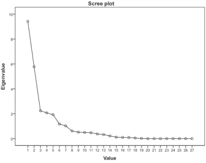
The number of independent variables is first reduced with the help of the PCA to identify the important ones which will used in the model. Scree plot shows the total variance associated with each factor. The point where the slope of the curve is clearly leveling off indicates the number of factors that should be generated by the analysis. PCA gives 7 factors as seen in the scree plot (Fig. 1).
Different methods are used to determine the appropriate number of factors. The researcher can determine the appropriate number of factors [36] by looking at eigenvalue and scree plot. The ones with eigenvalue above 1 in scree plot are taken into account. Those with eigenvalues less than 1 are not considered to be stable [29]. This is a value that SPSS automatically assign. However, researchers can increase or decrease the value subjectively. In this study, components with eigenvalue greater than 1 are taken into account [29, 36] in accordance with the standard. The total variance explained ratio is 87.504%. The Total Explained Variance table is given in (Tab. II) and Rotated Component Matrix in (Tab. III). Period variable is regarded as dummy variable.
A total of 27 independent variables are included in the analysis. Here, a cor-relation value above 0.60 is deemed important. For this set of variables, there are 26 correlations satisfying this requirement. Accordingly, the variables included in the analysis are: assets size, assets quality, gold bar, open market repurchase transactions, off-balance sheet transactions, credit risks, fixed assets, annual in-flation rates, non-interest income, non-interest expenses, interest expense, interest incomes, income-expense structure, annual real GDP growth rate, BIST 10 bank
Initial eigen v alues Extraction Sums of Squared Loadings Rotation Sums of Squared Loadings Comp onen t T otal % of V ariance Cum ulativ e % T otal % of V ariance Cum ulativ e % T otal % of V ariance Cum ulativ e 1 9.424 34.902 34.902 9.424 34.902 34.902 8.108 30.030 30.030 2 5.775 21.388 56.290 5.775 21.388 56.290 5.551 20.558 50.587 3 2.234 8.274 64.564 2.234 8.274 64.564 3.056 11.318 61.905 4 2.070 7.667 72.232 2.070 7.667 72.232 2.544 9.423 71.328 5 1.927 7.137 79.369 1.927 7.137 79.369 1.673 6.197 77.525 6 1.172 4.343 83.711 1.172 4.343 83.711 1.467 5.432 82.956 7 1.024 3.792 87.504 1.024 3.792 87.504 1.228 4.547 87.504 8 0.614 2.273 89.777 9 0.516 1.912 91.689 10 0.492 1.822 93.511 11 0.473 1.754 95.264 12 0.376 1.391 96.656 13 0.325 1.205 97.861 14 0.215 0.798 98.659 15 0.115 0.426 99.085 16 0.096 0.356 99.441 17 0.088 0.326 99.767 18 0.046 0.171 99.939 19 0.017 0.061 100.000 20 4.788E-15 1.773E-14 100.000 21 2.505E-15 9.277E-15 100.000 22 1.942E-15 7.194E-15 100.000 23 8.390E-16 3.107E-15 100.000 24 3.849E-16 1.426E-15 100.000 25 -2.624E-17 -9.720E-17 100.000 26 -2.228E-15 -8.252E-15 100.000 27 -3.727E-15 -1.380E-14 100.000 Extraction Metho d: Principal Comp onen t Analysis. T ab. I I T otal varianc e explaine d.
Fig. 1 Scree plot displaying the eigenvalues associated with components.
index (XBN10), annual interest on deposits, cyclical outputs, loans / total assets, liquidity, securities, industrial production index, currency basket, capital adequacy, consumer price index, concentration and money supply.
4.3
The artificial neural network model configuration
There are certain issues that must be taken into account during the development of a software model of ANN. In particular, if there is a big difference of the digital quantities between the input values of the ANN problem, it may negatively affect the output of the network. In other words, data with different scales in ANN training generally cause the neural networks to be unstable and can also cause the accuracy limits of the computers to be exceeded. Data must be scaled at least to the range used by the input neurons in the ANN [48]. Therefore, the input values of the network are in general scaled to the range (-1, 1) or (0, 1). In this way, the data measured using different units are reduced to the same scale and the effect of the very big or very small digital values is removed. Scaling must be applied prior to the commencement of the training process.
The mathematical expression for the software code used in the scaling is y = (ymax− ymin)(x− xmin)
(xmax− xmin) + ymin
(1)
where ymax represents the maximum value of column y; ymin represents the min-imum value of column y, while the xmax and xmin represent the maximum and minimum threshold values of the dataset respectively, and y represents the scaled
Component 1 2 3 4 5 6 7 Banks −0.086 0.371 −0.058 0.552 0.144 0.564 −0.167 FIA 0.027 −0.295 −0.827 0.053 0.117 0.115 −0.055 IES 0.016 0.163 0.030 −0.260 −0.115 0.695 0.553 DEP −0.218 0.716 0.138 0.114 0.011 −0.013 0.422 INF −0.942 −0.213 −0.061 −0.007 −0.008 0.006 −0.002 CON 0.832 0.146 −0.043 0.145 −0.439 0.008 −0.001 GDP −0.892 −0.208 −0.074 0.011 −0.062 0.009 0.000 BIST 0.968 0.214 0.046 0.010 0.006 −0.002 0.008 CYO −0.336 0.191 0.764 0.121 −0.140 −0.168 −0.056 SEC 0.630 0.197 0.153 −0.205 0.695 −0.014 0.021 IIN −0.651 0.110 0.058 0.205 0.289 −0.052 −0.064 IEX 0.802 −0.456 −0.081 0.065 −0.078 −0.018 −0.102 NIE 0.820 0.152 −0.135 0.370 −0.019 −0.035 −0.050 CRE −0.237 0.892 0.254 −0.098 −0.145 0.035 −0.094 IPI −0.053 −0.352 0.078 0.589 0.086 −0.258 0.601 NIR 0.720 0.232 −0.345 0.450 0.024 −0.145 −0.250 LIQ 0.267 −0.887 0.015 −0.007 0.070 −0.087 0.150 CAA 0.179 −0.728 0.556 −0.055 −0.061 0.154 −0.083 AS −0.957 −0.198 −0.020 −0.066 0.182 0.001 −0.001 AQ −0.237 0.892 0.254 −0.098 −0.145 0.035 −0.094 LTA 0.197 −0.718 0.220 0.065 −0.102 0.021 0.119 MS −0.085 0.343 0.071 0.831 0.198 −0.164 −0.016 SES 0.076 0.406 −0.194 −0.506 −0.232 −0.417 0.237 CUR 0.179 −0.728 0.556 −0.055 −0.061 0.154 −0.083 OBS −0.951 −0.194 −0.014 −0.075 0.212 0.000 −0.001 BG 0.703 0.190 0.100 −0.139 0.489 −0.004 0.025 AID 0.916 0.177 −0.007 0.110 −0.328 0.002 −0.003 OMR 0.592 0.174 0.156 −0.238 0.707 −0.020 0.048 Extraction Method: Principal Component Analysis.
Tab. III Component matrix.
values in the range (−1, 1). Since hyperbolic tangent is used as ANN activation function, the data are scaled to the range (−1, 1).
To analyze how ROA and ROE of banks are explained by the independent vari-ables shown in Tab. I, an ANN model is established by means of MLP architecture [55]. Many studies, which are considered as successful, imply that there is no stan-dard method for the determination of parameters concerning the network structure [11, 21, 23, 42, 56]. But these studies also discuss that parameter identification can be performed based on the problem area and data or on prior self-experience, rec-ommended settings in the literature or trial and error method adoption [21, 23, 43]. By taking this situation into consideration and the experiences of other researchers who carried out studies, the network parameters which provide optimal results and performance were determined. As measures of performance, Mean Square Error (MSE), one of the most referenced measures of accuracy in literature, as well as
Mean Absolute Percentage Error (MAPE) values were used [10, 27, 35, 57, 62]. The criterion for stopping training is when the model reaches an MSE value under 0.01.
The path followed for constituting network structure, and the ultimate struc-ture is as follows: The number of processing elements in the input layer has been defined as 27 following the number of input parameters. In the output layer, there is one neuron. A three layer network structure containing one hidden layer has been frequently used in previous studies estimating financial data [33, 34, 35, 62]. Ac-cordingly, considering appropriate literature and expert opinions, one hidden layer has been considered as sufficient. Here, in order to determine other parameters of the network infrastructure that will provide the best estimation performance, training data have been entered. The scaling of the data has been performed before training, as previously mentioned. In the trial period, the optimal values of three parameters are determined: the number of processing elements in the hidden layer, the learning coefficient and momentum coefficient. Firstly, the learning coefficient is determined as 0.1, and the momentum coefficient is determined as 0.9. While these two values are fixed, the numbers of hidden layer processing elements ranging from 1 to 55 are tried, and the performance values are recorded. 55 is the result of the formula [35, 46, 51] 2n + 1, where n is the number of processing elements in the input layer. Then, the number of hidden layer processing elements with the best value among these performance results is saved. Secondly, while the momentum coefficient is fixed, the number of hidden layer processing elements is the number saved in the first step, the network has been run separately for learning coefficient values ranging from 0.1 to 0.9, and the learning coefficient of the best performance is saved. Thirdly, while the number of hidden process elements determined in the first step, and the learning coefficient determined at the second step are fixed, the network has been run separately for each value of the momentum coefficient ranging from 0.1 to 0.9, and the learning coefficient of the best performance is saved. Finally, with the identification of parameters determined in the mentioned three-stage process by looking at the trial with the lowest error, optimizing the parameters of the network is completed.
In case of over-fitting or overtraining in the data validation of the ANN model, the data needs to be repartitioned [23]. Accordingly, depending on the results of the feedback, and model training obtained through the data validation phase, the data may need to be rearranged. In this case, since the training result of the neural network is not considered to be sufficient, it is decided to repartition the data. After the data are repartitioned into testing and validation, the learning process restarts. In this study, the training set contains sixty percent (60%) of the collected data, while each of the validation and testing sets contain twenty percent (20%) which are defined as optimal for LM–BP [25]. These percentages are obtained by repartitioning the data as a result of the comparisons and assessments during the feedback of the modeling outputs. The feedback is based on the MSE, and MAPE values. Therefore, a portion of twenty percent (20%) of the dataset used in the study is utilized for verification purposes.
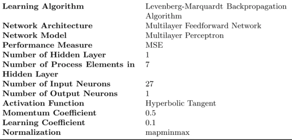
The details of the ANN model which is structured based on the mentioned optimal parameters, are provided in Tab. IV. The ANN structure is developed by coding in Matlab 2010 Editor. The ANN model is shown in Fig. 2.
Learning Algorithm Levenberg-Marquardt Backpropagation Algorithm
Network Architecture Multilayer Feedforward Network
Network Model Multilayer Perceptron
Performance Measure MSE
Number of Hidden Layer 1
Number of Process Elements in Hidden Layer
7
Number of Input Neurons 27
Number of Output Neurons 1
Activation Function Hyperbolic Tangent
Momentum Coefficient 0.5
Learning Coefficient 0.1
Normalization mapminmax
Tab. IV Details of the ANN model.
Fig. 2 Structure of the ANN model.
As is seen in Fig. 2, the input layer of the network has 27 neurons, which is the number of the input parameters. The output layer has one neuron. There is a single hidden layer and this layer contains 7 process components. Number of process components and number of PCA components are same, but this situation may be a coincidence. The weight matrices of the connections between each layer and the net input matrices corresponding to each neuron on each layer are indi-vidually obtained. The connection weights between the input layer and the hidden layer are represented by Wij (i = 1, 2, . . . , 27) (j = 1, 2, . . . , 7) and the connection weights between the hidden layer and the output layer are represented by Wjk (j = 1, 2, . . . , 7) (k = 1). The net input is simplified as the sum of the results obtained by multiplying all inputs with the weights corresponding to one neuron. Hi(i = 1, 2, . . . , 7) represents the net input corresponding to the hidden layer neu-ron and, I1 represents the net input corresponding to the output layer neuron. Y1 represents the output produced on the output layer.
4.4
Analysis and findings
The ROA performance of the neural network trained by the LM is shown in Fig. 3. The performance diagram is composed of three lines, since data are divided into three sets. The training set is represented by the blue line, the validation set by the green line and the testing set by the red line. As shown in Fig. 3, the network achieved a near-zero error at the 9th iteration. Since the error is reduced to below 0.01 as previously specified, the results are deemed acceptable. The training stopped at the 15th iteration, when the validation error started to increase.
0 5 10 15 10−3 10−2 10−1 100 101
Best Validation Performance is 0.0023823 at epoch 9
Me a n Sq u a re d Er ro r (m s e ) 15 Epochs Train Validation Test Best
Fig. 3 Best validation performance belongs to return on assets estimation.
No significant indication for over-fitting is observed until the 9th iteration, where the best validation performance appears; this is because the error rate in the validation, and testing set increases after that iteration. Since the testing set error and validation set error have similar characteristics and there is no significant indication for over-fitting, the network performance is deemed acceptable. On the other hand, the MSE value is important and examined for evaluating the perfor-mance of network. Various studies used the MSE value as a perforperfor-mance evaluation criterion of prediction and estimation with ANN on banking and financial domain. For example, Lavanya and Parveentaj [40] used Matlab neural network software as a tool to find the best algorithm for FOREX prediction by comparing the effective-ness of the back propagation algorithm and obtained an MSE value of 0.0035. In their previously mentioned study, Anyaeche and Ighravwe [10] constructed a back propagation model and obtained an MSE value of 0.02. Anastasakis and Mort [8] used Matlab Neural Network Toolbox 2.0 to find the best network topology by simulating an MLP network in order to predict the USD/GBP exchange rate and found a root MSE value of 0.1388306.
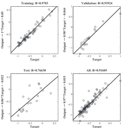
MSE indicates a value proportional to the difference between the estimated value and the actual values in the neural network. Here, the criterion for stopping training is when the model reaches an MSE value under 0.01. This value represents the maximum of difference between the estimated values and actual values would be 1%. In the literature [36], the values 0.05 and 0.01 is often used. In this study, the MSE result of the established model is observed as 2.3823× 10⁻³ for ROA estimation. Additionally, R correlation coefficient is used. R correlation coefficient is the measurement of how well the variations in the outputs are explained by the targets. R values closer to one indicate strong coherence, whereas values closer to zero indicate weak or no correlation. Fig. 4 shows the correlation between the outputs and the targets.
−1 −0.5 0 0.5 −1 −0.5 0 0.5 Target O u tp u t ~= 1*Tar ge t + 0.05 Training: R=0.9703 −1 −0.5 0 0.5 1 −1 −0.5 0 0.5 1 Target O u tp u t ~= 0.98*Tar ge t + − 0.044 Validation: R=0.93924 −1 −0.5 0 0.5 −1 −0.5 0 0.5 Target O u tp u t ~= 0.86*Tar ge t + − 0.022 Test: R=0.76638 −1 −0.5 0 0.5 1 −1 −0.5 0 0.5 1 Target O u tp u t ~= 0.97*Tar ge t + 0.015 All: R=0.91605
Fig. 4 Regression graph for return on assets estimation.
The training data represents a strong coherence. R correlation coefficient for the training data is approximately 1, and approximately 0.9 for the test and validation data. The scatter diagram is important since it shows that some data points represent a poor coherence. For example, the network output of some data in the testing set corresponds to 0.2, while the actual value is−0.5.
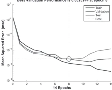
The ROE performance of the neural network trained by the LM is shown in Fig. 5. The training set is represented by the blue line, the validation set by the green line and, the testing set by the red line. As is shown in the Fig. 5, the network achieved a near-zero error at the 8th iteration. Since the error is reduced to
below 0.01 as previously specified, the results are deemed acceptable. The training stopped at the 14th iteration, when the verification error started to increase.
0 2 4 6 8 10 12 14 10−4 10−3 10−2 10−1 100 101
Best Validation Performance is 0.0026244 at epoch 8
Me a n Sq u a re d Er ro r (m s e ) 14 Epochs Train Validation Test Best
Fig. 5 Best validation performance belongs to return on equity estimation. No significant indication for over-fitting is observed until the 8th iteration, where the best validation performance appears, as the error rate in the valida-tion and testing set increases following that iteravalida-tion. Since the testing set error and the validation set error have similar characteristics and there is no significant indication for over-fitting, the network performance is acceptable. The MSE result of the model is observed as 2.624× 10⁻³, a value sufficiently small to achieve the determined target as previously discussed.
Fig. 6 shows the correlation between the outputs and the targets. If R value is closer to 1, it means there is a better coherence.
The training data represents a superior coherence, since R correlation coefficient for the training data is approximately 1. The test and validation outputs represent R values of approximately 0.9. The scatter diagram is important since it shows that some data points represent a poor coherence. For example, the network output of some data in the testing set corresponds to−0.4, while the actual value is −0.8.
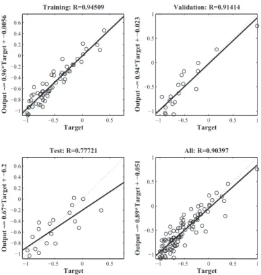
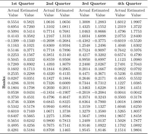
In the last one year period ROE of 24 commercial banks operating in Turkey decreased 2.42 percentage points to 8.67% while ROA decreased 0.44 percentage points to 1.10%. In one year, ROA and ROE of the entire groups of banks de-creased. According to the actual and estimated quarterly ROE and ROA values in Tab. V and Tab. VI respectively, average ROA was 0.38% (estimated ROA is 0.39%) and average ROE was 0.77% (estimated ROE is 2.88%) in the first quarter. In the second quarter, average ROA increased to 0.73% (estimated ROA is 0.71%) and ROE to 5.29% (estimated ROE is 5.24%). In the subsequent period, the aver-age ROA and ROE continued to increase. ROA occurred as 0.95% (estimated ROA
−1 −0.5 0 0.5 −1 −0.8 −0.6 −0.4 −0.2 0 0.2 0.4 0.6 Target O u tp u t ~= 0.96*Tar ge t + − 0.0056 Training: R=0.94509 −1 −0.5 0 0.5 1 −1 −0.5 0 0.5 1 Target O u tp u t ~= 0.94*Tar ge t + − 0.023 Validation: R=0.91414 −1 −0.5 0 0.5 −1 −0.8 −0.6 −0.4 −0.2 0 0.2 0.4 0.6 Target O u tp u t ~= 0.67*Tar ge t + − 0.2 Test: R=0.77721 −1 −0.5 0 0.5 1 −1 −0.5 0 0.5 1 Target O u tp u t ~= 0.89*Tar ge t + − 0.051 All: R=0.90397
Fig. 6 Regression graph for return on equity estimation.
is 0.95%) and ROE as 7.19% (estimated ROE is 7.45%). For the final quarter, the average percentage rate of ROA and ROE again increased compared to the third quarter. ROA occurred as 1.12% (estimated ROA is 1.11%) and ROE as 8.67% (estimated ROE is 8.46%).
By looking at the periodic change of the data in Tab. V and Tab. VI and other data available, some other conclusions can be reached. Considering development of non-interest income/expense on the basis of quarter periods, non-interest income decreased in the first three quarters of 2013, despite the increase in the last quarter. On the other hand, non-interest expenses which decreased in the third quarter, began to increase in the fourth quarter despite the downward trend in provisions. Therefore, despite the increase in net interest income, the decrease in non-interest expense coverage ratio of non-interest income has a negative effect on profitability in the final quarter. Despite the increase in net interest income in the fourth quarter, non-interest income/expense balance declined during this period. Another consequence of the model is that this movement adversely affected profitability rates. The amount of profit derived gradually decreased from the second quarter of the year. The main reason for the decline in the quarterly net profit in the second and third quarters is the decline in net interest income in these periods. However, rising interest rates in the second and third quarters had a negative impact on profitability.
1st Quarter 2nd Quarter 3rd Quarter 4th Quarter
Actual Estimated Actual Estimated Actual Estimated Actual Estimated Value Value Value Value Value Value Value Value
Banks 0.5554 0.5821 1.0616 1.0656 1.3008 1.2883 1.6012 1.9907 0.6954 0.7260 1.3102 1.0811 1.4325 1.1552 1.2319 1.3722 0.5094 0.5414 0.7714 0.7681 1.0463 0.8666 1.4796 1.7753 0.4143 0.3582 1.2167 1.3133 1.6034 1.6898 2.0753 2.8400 −0.1399 −0.1340 −0.2698 −0.2684 −0.4382 −0.3775 −0.6019 −0.5520 0.1163 0.1021 0.8369 0.9594 1.2548 1.2496 1.4046 1.6302 0.5146 0.3771 0.7718 0.7896 0.7524 0.9097 0.7642 0.5976 0.2253 0.1567 0.3851 0.3140 0.4217 0.3202 0.6574 0.4790 0.5045 0.4332 0.8559 0.9508 0.9950 0.8997 1.1123 1.0980 0.7289 0.8902 1.4393 1.8079 2.2400 2.0267 2.7491 2.7043 0.1602 0.1713 0.1844 0.2065 0.2014 0.1667 0.0822 0.0792 0.2535 0.2288 0.4320 0.4135 0.4471 0.3671 0.5236 0.4393 0.0287 0.0351 0.1827 0.1884 0.2646 0.2171 0.4855 0.5532 0.4286 0.3191 0.7326 0.6009 0.7344 0.7312 1.1227 1.0385 0.1804 0.1708 0.2030 0.2011 1.3463 1.6228 1.1381 1.4451 0.0538 0.0434 −0.1834 −0.1907 −0.2018 −0.2084 0.0044 0.0042 0.3750 0.4531 0.4796 0.4647 0.3574 0.3243 0.3503 0.3178 0.3746 0.3308 0.6845 0.8325 0.8364 0.7900 1.0018 1.0800 0.5342 0.5178 0.9940 0.8954 1.3159 1.1327 1.6046 1.6250 0.6010 0.7169 1.0671 1.3738 1.3279 1.3580 1.5265 1.8057 0.6407 0.5665 1.2275 1.3586 1.5647 1.1894 1.9657 1.8458 0.5654 0.6242 0.9800 0.7813 1.2409 1.0137 1.5028 1.7877 0.4895 0.4256 0.7675 0.7141 0.9146 1.0922 1.1702 1.0892 0.4281 0.5184 0.8708 1.1465 1.9545 1.8146 2.1514 1.9804
Tab. V Return on assets on quarterly basis.
By looking at the development of interest income/expense item on the basis of the quarterly periods, the first two quarters of declining interest expenses had a positive effect on profitability, but the upward trend in the last two quarters put downward pressure on profitability. However, the rise in interest income/expense ratio compared to the third quarter, due to the increase in interest income in the final quarter, contributed positively to profitability.
Asset size tended to increase until the fourth quarter as of the second quarter. However, the increase in deposits and securities, especially in the fourth quarter, affected asset size. Hence it is understood that deposits and issued securities are used for active funding. In the final quarter, the negative impact of the increase in foreign exchange losses on the net profit, though limited to some extent by derivative transactions and securities trading profit, put downward pressure on profitability.
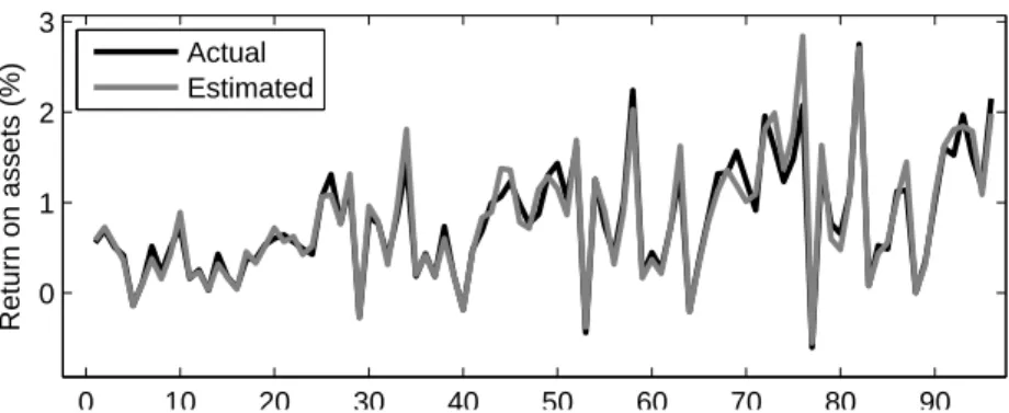
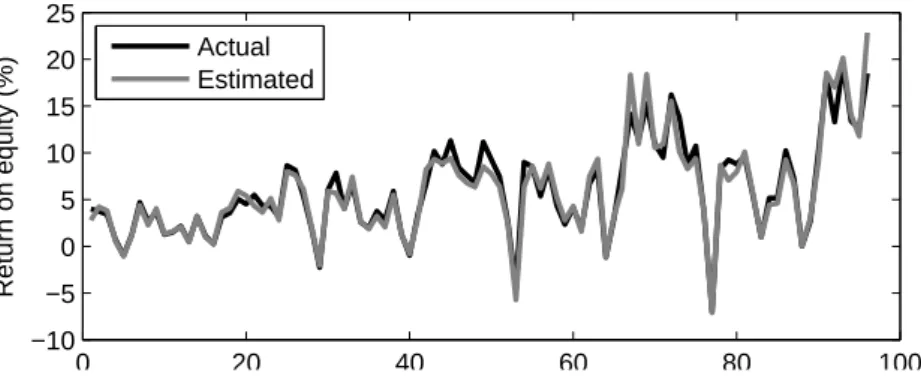
Referring to the results of the model, these two dimensions of profitability mea-surement (ROA and ROE) show parallelism with each other. Variations between the actual values with the estimated values listed in Tab. V and Tab. VI are shown in Fig. 7 and Fig. 8, respectively. Therefore, it can be concluded that the consis-tency between estimated values and actual values is high.
1st Quarter 2nd Quarter 3rd Quarter 4th Quarter
Actual Estimated Actual Estimated Actual Estimated Actual Estimated Value Value Value Value Value Value Value Value
Banks 3.9991 2.7966 8.6295 7.9946 11.1480 8.5150 13.7870 10.1133 3.7449 4.2344 8.1431 7.6160 9.2634 7.7575 8.7576 8.2768 3.3909 3.8017 5.3844 6.1355 7.4573 6.4133 10.7342 9.3578 0.7348 0.5235 1.9548 2.0997 2.6803 2.3855 3.6736 3.8044 −0.9697 −1.0630 −2.2507 −2.0319 −4.4017 −5.7097 −6.9904 −7.0972 1.2068 1.1194 6.0400 5.8940 9.0001 6.3954 8.2946 8.6751 4.6914 4.3579 7.8489 5.6875 8.5121 8.5996 9.2403 7.0728 2.6161 2.2626 4.0508 4.0104 5.3776 6.2126 8.8119 7.9502 3.6970 4.0418 6.7604 7.4267 8.3636 8.7954 9.5998 10.0969 1.2728 1.3273 2.5769 2.6513 4.3986 5.2527 5.3849 5.6094 1.4934 1.5965 2.0025 1.8436 2.3351 2.7831 0.9878 0.9726 2.1626 2.0657 3.7589 3.2475 4.1218 4.2900 5.1552 4.4338 0.5121 0.4721 2.8206 2.0667 1.8954 1.5890 5.1592 4.5884 3.2198 3.1989 5.8979 5.4809 6.6984 7.4759 10.2274 9.2422 1.1247 0.9925 1.3047 1.2812 8.2358 9.3439 7.2957 6.6683 0.2584 0.3089 −0.9712 −0.7776 −1.1899 −1.1242 0.0291 0.0305 3.1108 3.6242 3.4600 3.0697 3.0009 3.2535 2.6676 3.0309 3.5683 4.0808 6.6465 8.1943 8.2976 6.1423 10.1212 9.0046 5.0449 5.8831 10.1618 9.3171 14.1669 18.3440 18.1310 18.5447 4.5363 5.4289 8.7874 8.8733 11.4111 10.9680 13.3078 16.9937 5.5014 4.3273 11.2923 9.4140 15.2734 18.3931 19.4464 20.1413 4.3578 3.6401 8.4287 7.5950 10.9555 10.5463 13.4160 14.0588 4.2918 5.1419 7.5808 6.7741 9.5040 10.9163 12.5674 11.7840 3.1490 2.8132 6.8031 6.3407 16.2064 15.5108 18.5048 22.8404
Tab. VI Return on equity on quarterly basis.
0 10 20 30 40 50 60 70 80 90 0 1 2 3 Return on assets (%) Actual Estimated
Fig. 7 Variances between actual and estimated values of return on assets.
According to the results, the R correlation coefficient values indicate that the variation in the outputs is sufficiently explained by the targets. In addition, the co-efficient of determination values indicate that the coherence between the estimated
0 20 40 60 80 100 −10 −5 0 5 10 15 20 25 Return on equity (%) Actual Estimated
Fig. 8 Variances between actual and estimated values of return on equity.
and target values is high at the optimal iteration. Based on the great performance of the model, it is seen that the 26 explanatory variables included in the analysis are superior [3, 4, 12, 14, 26, 37, 49, 54] for the explanation of ROA and ROE. Considering that there are countless measurable and immeasurable factors that affect ROA and ROE, this value obtained from this study is exactly valuable for banks.
5.
Conclusion
This study is intended to analyze the impact of the internal (bank specific) and external (sectoral and macroeconomic) economical indicators on ROA and ROE of 24 deposit banks operating in Turkey. There are numerous classical regression and neural network studies using bank data. Various statistical assumptions are found in multiple linear or nonlinear regression studies. Studies, which do not met these assumptions, may not be reliable. In addition, it is difficult to implement such models as the number of variables increase. Therefore, the analysis performed by such methods can be applied successfully for limited applications. Consequently, this article is intended to analyze the profitability of deposit banks in Turkey with an adaptive software model of ANN which has not been previously applied in this context, comprehensively.
The results from the study indicate that ANNs are tools with great capabil-ity of generalization and thus estimation. According to software model results, the correlation coefficient R values show that variations in output are explained well by the targets. Moreover, the coefficients of determination values also show that the harmony between the estimated values of the network with the actual values is ex-cellent at the best iteration. Consequently, the results from the model indicate that all of the explanatory variables used have significant impact in varying proportions on profitability and that obtained estimations achieved the targeted and acceptable performance of success. In addition, the software model of ANN designed and the profitability estimation performed by the model are objective, highly steady and strong against user changes since they are transparent and not based on intuitive observation or expert opinions. This software model is not affected by the user differences, makes successful estimations and will facilitate the estimation of bank
profitability. Due to this and other successful results, this software model provides banks with the opportunity to estimate their profitability and researchers may also benefit from the great opportunity afforded by the ANN model.
In light of the findings of this study, the intelligent software model, which mea-sures bank profitability through the soft computing techniques, is able to estimate the profitability of banks at any time upon the insertion of the then-current data to the model, and thus provides a great tool for estimation studies. In addition, it has the capability to adapt to changing conditions and improve upon its already user-friendly structure to best respond to the requirements and expectations of researchers. The periodicity of the bank data between the years is a subject of another study. In this context, it is planned to perform panel data analysis by adding the data of 2014 and 2015 in a future work.
References
[1] ACARAVCI S.K., CALIM, A.E. Turkish banking sector’s profitability factors [online].
In-ternational Journal of Economics and Financial Issues. 2013, 3(1), pp. 27–41 [viewed
2014-10-20]. Available from: http://www.econjournals.com/index.php/ijefi/article/view/343/pdf [2] AKKOC S. An empirical comparison of conventional techniques, neural networks and the three stage hybrid adaptive neuro fuzzy inference system (ANFIS) model for credit scoring analysis: The case of Turkish credit card data. European Journal of Operational Research. 2012, 222(1), pp. 168–178, doi: 10.1016/j.ejor.2012.04.009.
[3] ALBERTAZZI U., GAMBACORTA L. Bank profitability and the business cycle. Journal of
Financial Stability. 2009, 5(4), pp. 393–400, doi:10.1016/j.jfs.2008.10.002.
[4] ALPER D., ANBAR A. Bank specific and macroeconomic determinants of commer-cial bank profitability: empirical evidence from Turkey [online]. Business and
Eco-nomics Research Journal. 2011, 2(2), pp. 139–152 [viewed 2014-10-20]. Available from:
http://papers.ssrn.com/sol3/papers.cfm? abstract id=1831345
[5] AL–QAHERI H., HASSANIEN A.E., ABRAHAM A. Discovering stock price prediction rules using rough sets. Neural Network World. 2008, 18(3), pp. 181–198.
[6] ALTAS D., CILINGIRTURK A.M., GULPINAR V. Analyzing the process of the artifi-cial neural networks by the help of the soartifi-cial network analysis [online]. New Knowledge
Journal of Science. 2013, 2(2), pp. 80–91 [viewed 2014-11-20]. Available from: http://
http://uard.bg/files/custom files/files/documents/New%20knowledge/year2 n2/paper altas y2n2.pdf
[7] ALTUNOZ U. Bankaların finansal ba¸sarısızlıklarının yapay sinir a˘glarımodeli ¸cer¸cevesinde tahmin edilebilirli˘gi [online]. Dokuz Eyl¨ul ¨Universitesi ˙Iktisadi ve ˙Idari Bilimler Fak¨ultesi Dergisi. 2013, 28(2), pp. 189–217 [viewed 2014-11-20]. In Turkish. Available from: http://iibf.deu.edu.tr/deuj/index.php/cilt1-sayi1/article/download/342/pdf 308
[8] ANASTASAKIS L., MORT N. Neural network–based prediction of the USD/GBP exchange
rate: the utilisation of data compression techniques for input dimension reduction
[on-line]. University of Sheffield, 2000 [viewed 2014-10-30]. Technical Report. Available from: http://www.researchgate.net/ profile/Leonidas Anastasakis/publications
[9] ANI W.U., UGWUNTA D.O., EZEUDU I.J., UGWUANYI G.O. An empirical assessment of the determinants of bank profitability in Nigeria: bank characteristics panel evidence.
Journal of Accounting and Taxation. 2012, 4(3), pp. 38–43, doi: 10.5897/JAT11.034.
[10] ANYAECHE C.O., IGHRAVWE D.E. Predicting performance measures using lin-ear regression and neural network: a comparison. African Journal of Engi-neering Research. 2013, 1(3), pp. 84–89 [viewed 2014-09-20]. Available from: http://www.netjournals.org/z AJER 13 028.html