Effect of load, processing time and due date variation on the effectiveness of scheduling rules

(1)

Full Terms & Conditions of access and use can be found at

http://www.tandfonline.com/action/journalInformation?journalCode=tprs20

Download by: [Bilkent University] Date: 13 November 2017, At: 03:01

International Journal of Production Research

ISSN: 0020-7543 (Print) 1366-588X (Online) Journal homepage: http://www.tandfonline.com/loi/tprs20

Effect of load, processing time and due date

variation on the effectiveness of scheduling rules

Tahar Lejmi & Ihsan Sabuncuoglu

To cite this article: Tahar Lejmi & Ihsan Sabuncuoglu (2002) Effect of load, processing time and due date variation on the effectiveness of scheduling rules, International Journal of Production Research, 40:4, 945-974, DOI: 10.1080/00207540110098481

To link to this article: http://dx.doi.org/10.1080/00207540110098481

Published online: 14 Nov 2010.

Submit your article to this journal

Article views: 53

View related articles

(2)

E ect of load, processing time and due date variation on the e ectiveness

of scheduling rules

TAHAR LEJMI and IHSAN SABUNCUOGLU *

In real manufacturing environments, variations in production factors (i.e. pro-cessing time, demand, due-dates) are inevitable facts. All these dynamic changes, together with random disturbances (e.g. machine breakdowns) can seriously a ect the system performance. In this paper we focus on load, processing time and due date variation and analyse their impacts on a scheduling system. Speci®cally, we investigate the impact of variation on dispatching policies in a job shop environ-ment via simulation. The statistical analysis of the results leads to two major conclusions: ®rst, the relative performance of rules is not threatened much by PV (processing time variation), LV (load variation) or DDV (due date variation) Ð a result that can be a consolation for practitioners in the ®eld. Secondly, the performance of the rules deteriorates, in particular at high levels of PV, LV and DDV Ð a result that can provide new insights into the problem and produces useful information for researchers in their continuous e ort to develop better dispatching rules.

1. Introduction

The job-dispatching environment often requires the use of processing time esti-mates that are usually subject to error. An anticipated processing time is generally based on a best estimate, which is sometimes an average of the actual processing times from the previous job processing operations. In practice, the estimation of this true processing time is a di cult task due to various random factors involved in production environments (e.g. variations in machining conditions, operator, material, etc). In addition, actual processing times often di er from their estimated values due to these random factors.

For the last four decades, scheduling problems have been extensively studied in the literature. In most of the existing studies, however, randomness in processing times is not fairly incorporated in the models. In deterministic studies that constitute the majority of existing scheduling work, processing times are considered as known quantities or parameters of the problem and the best schedule is developed to opti-mize some performance measure (e.g. makespan, mean tardiness, mean ¯ow time). In practice, however, the actual performanc e and events (start and completion times of jobs) can be signi®cantly di erent from so-called predicted (or planned) perform-ance due to various random events. For that reason, the pre-determined optimum schedules may not always yield the best results. This highlights an important point

International Journal of Production Research ISSN 0020±7543 print/ISSN 1366±588X online # 2002 Taylor & Francis Ltd http://www.tandf.co.uk/journals

DOI: 10.1080/00207540110098481

Revision received May 2001.

{ Department of Business Administration, Bilkent University, 06533 Bilkent, Ankara, Turkey.

{ Department of Industrial Engineering, Bilkent University, 06533 Bilkent, Ankara, Turkey.

* To whom correspondence should be addressed. e-mail: sabun@bilkent.edu.tr

(3)

that one should measure the deviation between the planned and realized schedules, and its impact on system performance.

Researchers have also developed stochastic scheduling models to cope with ran-domness in production environments. Generally speaking, stochastic problems are more di cult than their deterministic versions. In stochastic formulations, well-known probabilistic distribution functions (e.g. normal, exponential) are assumed for processing times and jobs are scheduled using the expected quantities (e.g. mean processing times of jobs etc). The best schedule is determined so as to optimize the expected value of some performance measure (i.e. the expected sum of completion times). Even though the stochastic approach brings some realism to the scheduling systems, the optimum schedule generated by the stochastic models may not be totally di erent from the deterministic models. As shown by Pinedo (1995) in the single machine scheduling environment, the optimum schedule for deterministic problem may also optimize the objective of the stochastic version. Regardless of whether the schedules are generated by deterministic or stochastic models, the actual perform-ance of the systems can be considerably di erent than the planned performperform-ance. Except for a few studies, this important deviation has not been thoroughly studied in the literature. We investigate this issue in this paper.

Since most scheduling problems (even the simple ones with static and determi-nistic assumptions) are NP-hard, researchers in the literature have frequently employed simulation to model the stochastic and dynamic nature of scheduling systems and to test the performanc e of various heuristics or scheduling rules. In most of these applications, processing times are sampled from random distribution functions, but these sampled quantities are used in scheduling decisions as if they are deterministic. Thus, actual (or true) processing times of jobs are assumed to be the same as expected (or anticipated) processing times. This assumption usually does not ®t real situations, and there is always deviation between planned and actual perform-ances. Hence, it is useful to examine the e ects of the deviation between true and anticipated processing times on the performance of scheduling systems.

Another source of variability in practice is the workload variation that might have negative e ects on the scheduling performance. The source of variability is due to the fact that the system itself experiences changes in demand over time. This can be observed in real situations where demand depends on external factors that cause its ¯uctuation over time. Despite the fact that variation in workload may a ect system performance, scheduling problems have usually been studied in environments where uniform workload is assumed. This assumption may not ®t all real situations. Therefore, it is also important to study the e ect of workload variation on the e ectiveness of scheduling systems.

In real job shop environments, job due dates, although ®xed before jobs go on process, may undergo changes after. This can be observed in real situations where, due to some external or internal factors, manufacturers have to ®nish a job before or after its originally set due date. We expect that the variations that job due dates can undergo during the jobs processing, can have considerable negative impact on the performance of priority rules. Nevertheless, we are not aware of any study that has considered the phenomenon. All studies in the literature have assumed that due dates do not change once they are determined.

In this paper, we study the Load Variation (LV), Processing Time Variation (PV), and Due Date Variation (DDV) and their e ects on the scheduling system. First, we test the scheduling rules for varying levels of PV. Here, PV is de®ned as the

(4)

deviation between a true and an anticipated processing time. Secondly, we consider load variation and analyse the performance of the scheduling rules under four dif-ferent LV schemes. Finally, we investigate the e ect of due date variation on the e ectiveness of priority rules. The objective is to uncover the e ect of PV, LV and DDV on the performance of priority rules for the mean ¯ow time (MF) and mean tardiness (MT) measures.

The rest of the paper is organized as follows. Section 2 presents a literature review. Section 3 gives the system considerations and experimental conditions. Section 3 also discusses modelling PV, LV and DDV. Results are presented in section 4. Finally, the paper ends with concluding remarks in section 5.

2. Relevant literature

2.1. Processing time variation

Research on the e ect of the deviation between true and anticipated processing times on priority rules performance is rare because the existing work on scheduling assumes ®xed and true processing times (Smith et al. 1973). Despite the fact that some variability of processing times is assumed in scheduling problems, this varia-bility in a research environment is due to drawing processing times from a prob-ability distribution function. The true processing times are usually assumed to be ®xed with no di erences between true and anticipated processing times. Our litera-ture survey indicates that a few works exist on this subject.

Pinedo (1982) studies the optimization problem of minimizing the completion time while taking into account the variability in job processing times from di erent machines in stochastic ¯ow shops. He concludes that, to minimize the expected makespan, jobs with smaller expected processing times and larger processing time variances should be scheduled either at the beginning or at the end of the schedule. The work done by Suresh et al. (1985) supports Pinedo’s conclusion. Pinedo and Weiss (1987) further develop the `Largest Variance First’ policy for minimizing both expected ¯owtime and expected makespan for stochastic scheduling problems. Frostig (1988) extends this study and generalizes the results of Pinedo and Weiss.

Smith et al. (1973) investigate the e ects of the uncertainty of processing time estimates on scheduling rule performance by using the SPT rule and the makespan criterion. The authors observe that the uncertainty of processing time estimates a ects the performance of the SPT rule in minimizing makespan. In another study, Yumin et al. (1994) examine the e ect of inaccuracy of processing time esti-mation on the e ectiveness of well-known dispatching rules (i.e. SPT, MST, EDD, FOPNR and MOPNR) for various measures such as mean ¯ow time, mean tardiness and proportion of tardy jobs. They conclude that when the inaccuracy of processing time estimation is not large, with a standard deviation of the true and anticipated processing times being 10, the inaccuracy does not signi®cantly a ect the perform-ance of the scheduling rules. However, at higher levels of inaccuracy, there is obvious deterioration of the performance of priority rules. They also observe that due-date based rules are more robust than non due-date based rules.

In another study, Sabuncuogl u and Karabuk (1999) investigate the frequency of scheduling in an FMS with uncertain processing times and unreliable machines. The results indicate that both machine breakdowns and processing time variation have negative e ects on the system performance. The authors also report that di erences between the optimum seeking algorithms and simple scheduling rules diminish as the level of variability in the system increases. Similar observations are also made by

(5)

Lawrence and Sewell (1997). In this study, the authors investigate the e ects of stochastic processing times on scheduling methods and ®nd that the ®xed optimum sequence is outperformed by simple heuristics or dispatching rules as the variability increases. Finally, Sabuncuoglu and Comlekci (1997) consider PV in the relative comparison of ¯ow time estimation methods. Their results indicate that the perform-ance of the ¯ow time estimation methods deteriorates at high PV levels.

2.2. Load variation

Similar to PV, most previous studies on scheduling rules ignore the possible variations of system workload over time. Researchers usually assumed uniform work load or (machine utilization) within their system models. Ramasesh (1990) who made a survey of simulation research on dynamic job scheduling, points out that most studies have been carried out at a single predetermined level of shop utilization. Carroll (1965) and Baker and Dzielinski (1960) employ an 80% level. Eilon and Chowdhury (1976) and Weeks and Fryer (1977) use a 90% level. Elvers (1973) uses heavily loaded shops with 97% utilization level.

In a later study, Elvers and Taube (1983) use six di erent levels of shop loading to evaluate the performance of various priority rules across a shop utilization spec-trum. Conway (1964) uses three utilization levels Ð 88.4, 90.4 and 91.9% Ð in his study. Hottenstein (1970) uses two levels of 72% and 94%. Note that most studies set utilization levels by adjusting the arrival rate parameter of the input process.

Among the studies that considered LV, Jones (1973) points out that one might expect that changing conditions associated with increasing demands for work from a job shop will be served best by changing the scheduling rules. The same conclusion is also reached by Elvers and Taube (1983) who compare the rank-order performance of ®ve scheduling rules against the criterion of `percentage of on time completion’. Their results indicate that the relative performance of the rules is dependent on the shop-load level. Sabuncuoglu and Comlekci (1997) test the e ect of LV on the ¯ow time estimation method in terms of ML (mean lateness), MT and MF criteria. In this study, LV is achieved by varying randomly the arrival rate of the jobs so that the load level ¯uctuates within a certain margin of the average load level of the system. The results indicate that the performance of the ¯ow time estimation method is quite robust to LV. Speci®cally, two LV levels are considered: 10% and 20%, and at neither level has the ¯ow time estimation method performance been a ected con-siderably.

2.3. Due date variation

To the best of our knowledge there is not even a single study in the literature that examines the due date variation in the scheduling context.

3. System considerations, simulation model and experimental conditions

3.1. Suggested model

In a dynamic and stochastic manufacturing environment, testing scheduling rules under di erent experimental conditions becomes a more complex task than in the static case. It follows from the fact that one should be very careful on the model choice. The generality aspect of such a model must be kept at a maximum in order to get potential bene®ts from the experiments. Our model is similar to the one used by Vepsalainen and Morton (1987). It is a re-entrant dynamic job shop model with:

(6)

. Ten machines are continuously available.

. Continuous arrival of jobs having a Poisson distribution.

. Number of operations assigned to each job arrived is random having a uni-form distribution U[1,10].

. Each operation is equally likely to be performed on ten machines, where pro-cessing times are random having a uniform distribution U[1,30].

The assumptions of this model are given in the study by Vepsalainen and Morton (1987).

3.2. System load (or machine and shop utilization)

The combined e ects of job arrival distribution, job routing and processing times determine system load (or the machine utilization). From the standpoint of job-shop simulation, machine utilization is important because it a ects queue lengths. If the average queue length is too small, the scheduling rules used in the model may not be forced to make discriminating job selections; when this situation occurs, an evalua-tion of rule e ectiveness is di cult or impossible. Adverse e ects also result from machine utilization when it is too high. If utilization is near 100%, transient con-ditions may extend over a long time period. Machine utilization commonly found in the literature ranges from 60% to 95%. This range of utilization permits scheduling rules to select a job from several in the queue but does not lead to very long queues. In our study, when analysing the e ects of PV and DDV, we consider two levels of machine utilizations: 60% (low) and 85% (high). In the LV case, however, we start with an initial 72.5% level (which corresponds to the medium utilization level) and change it according to the LV scheme under consideration by adjusting the arrival rate.

3.3. Due date tightness and assignment rule

Due date performances of the rules are a ected by due date tightness. In general, tighter due dates tend to produce larger values of MT (mean tardiness) and PT (proportion of tardy jobs), if other conditions remain unchanged (Carroll 1965). Beyond that there is also evidence that the relative performanc e of priority rules is also a ected by due date tightness, at least for PT and for MT. This suggests the existence of so-called cross-over points, with one rule performing best for tighter due dates and another performing best for looser due dates. In this study, we use the TWK approach in assigning the due dates. The reason is that the TWK method is found to be the most e cient rule to reduce the cross-over e ect (Baker 1984). According to TWK, job due dates are de®ned as follows:

Dj Rj Aj;

where, Aj k Pjrepresents the original ¯ow allowance, k is the due date tightness

value and Rj denotes the arrival time of job j.

Baker (1984) suggests that 10% and 40% PT values represent loose and relatively tight due dates respectively. These PT values are used as the reference values to apply due date tightness to the simulation experiments in almost all every study, except that we have lately performed some experiments at extremely tight due dates for the symmetric criterion, Mean Absolute Deviation (MAD). In order to set tight due

(7)

dates or loose due dates, the parameter k should be adjusted so that we achieve the desired PT values mentioned previously (i.e. 10% and 40% values). In this study, we use separate pilot runs to set the values of k, with respect to FCFS (benchmark rule) for di erent machine utilization levels. Note that the same value of k is used for all tested priority rules under the same utilization level.

3.4. Scheduling rules

According to previous studies, SPT (Shortest Processing Time) and MOD (Modi®ed Operation Due date) rules are considered the most e ective rules for completion time and tardiness based criteria. Note that SPT and MOD are described as local rules. We de®ne local priority rules as those that require information only about those jobs that are waiting at a machine, while global rules require additional information about jobs or machine states or other machines. STPT (Shortest Total Processing Time) and the MDD (Modi®ed job Due Date) rules can be considered as the global rules in this context. In this study we use these four rules. We believe that using local and global rules makes the results of the study more general and reliable. To seek further generality, we use two other local/global pairs of rules: ODD (Operation Due Date) and EDD (Earliest Due Date) rules, which are again simple but e ective rules. FCFS (First Come First Served) and FAFS (First Arrived First Served) rules are included as benchmark rules.

3.5. Performance criteria

In this study, we employ two scheduling performanc e measures: the mean ¯ow time (MF) and the mean tardiness (MT). The former criterion represents a speed of response in the manufacturing environment (lead-time) and is a good indicator of the production rate (or throughput). The latter criterion is a due-date based measure that measures the average level of customer satisfaction in terms of delivery perform-ance. These two are the most frequently used scheduling criteria in the literature.

3.6. Modelling PV

In order to model the processing time variation, we induce some perturbation in the processing times using the approach suggested by Sabuncuoglu and Comlekci (1997). That is, best estimates are drawn from the uniform distribution but only some percentages (plus or minus) of the sampled quantities are used as the actual processing times. The details are as follows:

pij 1 PV% UNIF 1; 1 pij;

where

pij estimated processing time value drawn from the uniform distribution,

pij true (actual) processing value, deviated from its estimated value,

PV% PV level percentage.

Seeking generality, we test with 0%, 20%, 40% and 60% PV% values. A point to note is that scheduling rules use estimated processing times to assign job priorities during the dispatching process, but when processing on machines occur, actual or true processing times are used to delay the operations.

(8)

3.7. Modelling LV

In real job-shop systems, due to some external factors, demand undergoes variation over time. This, in turn, causes the system workload to experience similar variation. In general, workload changes can occur in di erent ways. In our study, we consider four di erent schemes that would re¯ect most possible workload variation behaviours. The ®rst scheme represents a random change of workload over time. The second one is inspired from real situations where workload is seasonal. The last two alternatives consider the cases where workload is either continuously increasing or decreasing respectively. All these four load schemes are established by varying the arrival rate of the jobs to the system, as shown in the following four schemes.

Notation

¶ current arrival rate for current k jobs arrived, ¶ new arrival rate for next k jobs,

¶0 initial arrival rate, assigned at the beginning of each replication,

¶min lower bound for arrival rate,

¶max upper bound for arrival rate,

maximum increases or decrease range size. ¶max ¶min,

LV% a percentage value, a parameter that controls how much ¶ can maximally vary,

½ an increase/decrease index value, where

at the beginning of each replication, ½0 DISC. UNIF 1; 1

after that time, ½ is updated as follows: ½ 1 if ¶ < ¶min

1 if ¶ > ¶max;

n job batch size;

N total job number of jobs arriving per replication:

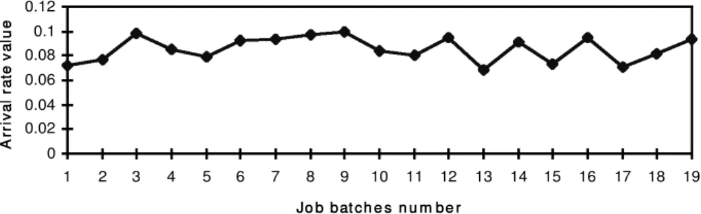
Scheme 1: (Random LV)

As illustrated in ®gure 1(a), the system workload level changes randomly over time. This is usually due to random demand (i.e. demand has no particular change pattern over time). In order to incorporate random LV to our model, whenever n jobs enter the system, the arrival rate ¶ is updated as follows:

¶ ¶0 UNIF LV% =2; LV% =2 : 0 0.02 0.04 0.06 0.08 0.1 0.12 1 2 3 4 5 6 7 8 9 10 11 12 13 14 15 16 17 18 19

Job batches num ber

A rr iv al r at e va lu e

Figure 1. (a) Illustration of random arrival rate.

(9)

Scheme 2: (Seasonal LV)

According to this LV scheme, demand is seasonal; that is, demand experiences a continuous increase/decrease followed by a continuous decrease/increase in repeated periodic cycles (see ®gure 1(b)). In order to incorporate seasonal LV to the model, we cause the arrival rate ¶ to change in such a way that it increases constantly until it reaches an upper bound level, then decreases again in a similar way until it reaches a lower bound level. This decrease/increase behaviour continues as far as jobs are entering the system. This approach is applied as follows.

0 0.02 0.04 0.06 0.08 0.1 0.12 1 2 3 4 5 6 7 8 9 10 11 12 13 14 15 16 17 18 19

Job Batches num ber

Figure 1. (b) Illustration of seasonal arrival rate.

0 0.02 0.04 0.06 0.08 0.1 1 2 3 4 5 6 7 8 9 10 11 12 13 14 15 16 17 18 19

Job Batches num ber

Figure 1. (c) Illustration of increasing arrival rate.

0 0.02 0.04 0.06 0.08 0.1 1 2 3 4 5 6 7 8 9 10 11 12 13 14 15 16 17 18 19

Job batches num ber

Figure 1. (d) Illustration of decreasing arrival rate.

(10)

At the beginning of each replication: initialize ¶ to ¶0.

After each n jobs arrived, ¶ is updated as follows:

¶ ¶ ½ UNIF 0; LV%

Scheme 3: (Increasing workload)

In this case, the arrival rate undergoes a positive variation after each n jobs arrival (see ®gure 1(c)). In the model, it is updated as follows:

Initially, ¶0 ¶min:

After then,

¶ ¶ UNIF 0; 3=2 n =N :

Scheme 4: (Decreasing workload)

In the ®nal case, we deal with real situations where demand is continuously decreasing (®gure 1(d)). The arrival rate in this case undergoes a negative variation (i.e. decrease) after each n jobs arrival and it is updated as follows:

Initially, ¶0 ¶max:

After then,

¶ ¶ UNIF 0; 3=2 n =N :

Numerical values PV

In the PV study, 60% and 85% are used as low and high machine utilizations. These levels correspond to arrival rate values of 1/14.5 and 1/10.3, respectively. Accordingly, the arrival rate bounds are determined as follows:

¶min 1=14:5;

¶max 1=10:3;

Accordingly:

¶max ¶min 1=10:3 1=14:5 0:028:

Seeking generality, the four approaches will be applied initially with a medium machine utilization environment: 72.5% level. The pilot runs indicate that the cor-responding arrival rate is 1/12. In the ®rst two LV schemes, at the beginning of every replication, the arrival rate is initialized to ¶0 1=12. Recall that we use the batch

means approach in the experiments. Every batch consists of N 900 jobs. For convenience, we assign n 45, which induces about 20 changes in the arrival rate in each replication. LV%, the parameter that controls how much ¶ can maximally vary will take two di erent values, 40% and 80%. In fact, when we increase the LV% value, we increase at the same time the LV rate.

3.8. Modelling DDV

As mentioned in section 3.3, the TWK method is used to set due dates in this study. In modelling this situation, each job is given a certain ¯ow allowance once it enters the system. As the job moves from one machine to another, with a certain probability p, it will undergo a change in its actual due date. Practically, in real job shops, a job will have its due date either postponed or made more urgent. This will depend on two major factors or players, the ®rst is the manufacturer side and the

(11)

second is the customer side. Therefore, two scenarios can occur: ®rst, if the job is expected to be late, or technically speaking, the job’s slack time is non-positive, than the manufacturer may be obliged to ask the customer to agree on postponing the job’s due date by a su cient amount of time (at least equal to its expected remaining manufacturing time). The next scenario occurs when the job is not to be late. In this case, the job’s slack time is positive. Consequently, the job due date can be either postponed or made more urgent. This can occur in real situations where the custo-mer needs the job to be ®nished either less or more urgently. Consequently, the manufacturer may agree to change the job due date, within some limitations that are set according to the actual status of the job. These two scenarios are de®ned as follows.

After ®nishing a certain operation of a job, with a small probability p.

(1) If its slack time at time t, Sj dj t Pj, where Pj is the remaining

opera-tion time) is positive, then the actual due date undergoes either a positive or negative change, which equals DV Sj, where DV is the due date variation

coe cient (which would range from 0.2 until 0.8).

(2) Otherwise, the job due date is postponed by being adding (1 0:5 DV Sj as a su cient time to ®nish the job.

A point worth noting is that the experimental factors that would be controlled during the study are:

. The probability of undergoing due date change p: a small value 0.05 will initially be used and then this will be increased to 0.10 to see the major e ects of increasing the due date change rate.

. The due date variation coe cient DV: this will range from 20%, 40%, 60% and 80%.

Of course, this approach could be more elaborate and improved, yet it will satisfy the goal of this study.

3.8.1. Due date variation analysis in terms of Mean Tardiness.

The expression for MT performanc e measure is as follows:

MT X n i 1 Tj n ; where,

Tj max Cj Dj; 0 ; job j tardiness;

Cj completion time of job j;

Dj due date of job j:

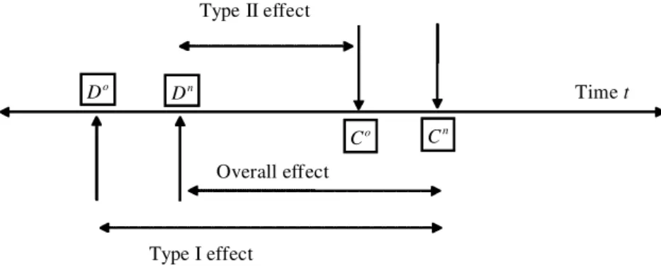
Once due date variation is included in the analysis, the MT performance of priority rules can change in terms of two main components. The ®rst is the com-pletion time of each job, Cj. Since the due dates of some jobs change, their relative

priority might change and, consequently, the completion times of jobs change. This e ect, due to changes, in Cjs is called the Type-I e ect. The second component is the

due date Dj. Recall that the tardiness is a function of due dates. Thus, as the due

dates of some jobs change, their tardiness values, in turn, change. This e ect is called

(12)

the Type-II e ect. The due date variation e ect due to these two components deter-mines the Overall e ect on the MT performance of the priority rules.

In fact, it is important to di erentiate between these three types of e ects. The Type-I e ect measures the new performance of the rule when it considers new due dates while assigning job priorities during the dispatching process. That leads to new completion times of the jobs in the process. However, the performance is measured in terms of the original due dates. In other words, the Type-I e ect can be viewed as the net e ect of due date variation on the dispatching policy performance. Note that non due-date based rules are insensitive to the Type-I e ect as they do not consider any due date information.

On the other hand, the Type-II e ect gives the new performance of the rules when they disregard any change in job due dates during the dispatching process. However, their MT performance is measured in terms of the ®nal due dates. A point to note is that non due-date based rules are only sensitive to this type of e ect, while due-date based rules are a ected by both e ects. The overall e ect is the combina-tion of these two e ects and re¯ects the global e ect of due-date variacombina-tion on the rule’s performance in terms of both changes in due date values and the dispatching policy performance.

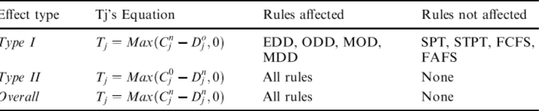
According to these three due date variation e ects, table 1 represents the corre-sponding tardiness (Tj) equations upon which the three e ects could be measured.

We also present the rules sensitive to such due date variation e ects. A graphical illustration of these type of e ects is shown in ®gure 2.

In fact, the Type II e ect simply measures the due date variation scheme that we adopt in terms of due date value changes, which is not of much concern to the scope of the study. Consequently, only Type-I and Overall e ects will be measured throughout the simulation experiments.

3.9. Output data analysis

The simulation model is developed using the SIMAN language (Pegden et al. 1995). The model is veri®ed and validated with reference to the hypothetical model suggested previously. The common random number variance reduction technique (CRN) is implemented to compare the rules under identical conditions and to reduce the experimental error. Initially, some pilot runs are taken to ®nd suitable values for the arrival rate to set the desired utilization levels. Two values are found for the

E ect type Tj’s Equation Rules a ected Rules not a ected

Type I Tj Max Cnj Doj; 0 EDD, ODD, MOD, SPT, STPT, FCFS,

MDD FAFS

Type II Tj Max C0j Dnj; 0 All rules None

Overall Tj Max Cnj Dnj; 0 All rules None

where,

C0j: Original (No due date variation) completion time of job j Doj: Original due date of job j

Cnj: New completion time of job j Dnj: Final due date of job j

Table 1. Corresponding Tjequations to due date variation e ect types.

(13)

arrival rate: 10.3 and 14.5, corresponding to 85% and 60% utilization levels, respect-ively. Furthermore, several other runs are also taken to estimate the warm-up period using the Welch approach discussed in Law and Kelton (1991). As a result, 300 job completions are deleted at the beginning of each run to reduce the e ect of initial bias. In order not to lose too much computer time, the batch means approach is used, ten batches of size 900 are analysed for each experiment run. For PV and DDV, pilot runs are also taken to set the parameter k for each machine utilization level, as shown in table 2. In the LV case, the same population of rules is tested in the experiments at the medium 72.5% utilization level for tight and loose due dates. According to pilot runs, the due date tightness factor k is set to 2.6 and 4.5, respect-ively.

4. Analysis of the simulation results

4.1. Results of processing time variation

Two classes of scheduling rules are tested in this study. The ®rst class consists of non due-date based rules: SPT, STPT, FAFS and FCFS. The second class includes due-date based rules: EDD, ODD, MOD and MDD. All rules are tested under three levels of PV: 20%, 40% and 60% and two performance measures, MF and MT. To seek generality, two system load levels (85% and 60%) as well as two due date tightness (tight and loose) levels are considered. The results of the simulation runs are presented in tables 3 and 4. The paired t-tests are applied to compare the best rule with the next best rule at a signi®cance level of 5%. The symbol (*) indicates when the di erence between the rules is signi®cant. In addition, the paired t-tests are also used to compare the performances of each rule as the processing time variation level (PV%) increases. The symbol (**) indicates that the di erence between original performance (no PV) and actual performance (with PV) is signi®cant. Figures 3

Do _Dn Co _Cn Type II effect Type I effect Overall effect Time t

Figure 2. Illustration of Type-I, Type-II and overall DV e ects.

Tight due dates Loose due dates High machine utilization (85%) k 4:5 k 7

Low machine utilization (60%) k 2 k 3

Table 2. Due date tightness parameter k values for PV.

(14)

and 4 are also provided to depict the behaviour of the system performance as a function of PV. From the analysis of the results, the following observations are made.

In all experimental conditions, SPT yields the best MF values. The second best performance is displayed by MOD and STPT. The latter rule performs especially well at the high utilization/loose due-dates condition. These two rules are followed by ODD, MDD and EDD. All these rules outperform the benchmark rules FCFS

Processing time variation Level %

0% 20% 40% 60%

High utilization (85%)/tight due-dates (k 4:5) SPT 261.52(*) 262.32(*) 268.86(*)(**) 281.94(*)(**) STPT 308.78 311.73 325.40(**) 323.17(**) FCFS 342.02 339.90 355.74(**) 373.47(**) FAFS 335.11 337.22 342.05(**) 366.85(**) EDD 318.31 318.71 324.08(**) 340.75(**) ODD 310.95 312.54 326.86(**) 336.78(**) MOD 300.47 301.38 312.11(**) 321.36(**) MDD 316.33 318.83 328.32(**) 338.34(**)

High utilization (85%)/loose due-dates (k 7)

SPT 261.52(*) 262.32(*) 268.86(*)(**) 281.94(*)(**) STPT 308.78 311.73 325.40(**) 323.17(**) FCFS 342.02 339.90 355.74(**) 373.47(**) FAFS 335.11 337.22 342.05(**) 366.85(**) EDD 314.21 317.21 325.80(**) 351.09(**) ODD 315.77 318.23 331.92(**) 335.01(**) MOD 314.68 315.99 324.47(**) 342.07(**) MDD 314.81 315.29 326.20(**) 342.26(**)

Low utilization (60%)/tight due-dates (k 2)

SPT 149.33(*) 150.39(*) 152.27(*) 156.76(*)(**) STPT 159.55 160.84 164.20(**) 167.50(**) FCFS 164.87 166.05 169.59(**) 174.44(**) FAFS 163.32 165.05 167.16 172.74(**) EDD 159.37 160.89 163.28 167.99(**) ODD 157.59 159.43 161.96 166.45(**) MOD 154.3 154.28 157.77 160.30(**) MDD 158.29 159.89 161.23 166.88(**)

Low utilization (60%)/loose due-dates (k 3)

SPT 149.33(*) 150.39(*) 152.27(*) (**) 156.76(*)(**) STPT 159.55 160.84 164.20(**) 167.50(**) FCFS 164.87 166.05 169.59(**) 174.44(**) FAFS 163.32 165.05 167.16 172.74(**) EDD 159.61 159.54 162.25 167.07(**) ODD 158.92 159.23 163.48 166.69(**) MOD 158.82 160.39 162.53 166.13(**) MDD 159.45 159.52 161.95 167.46(**)

(*) Statistically signi®cant at 5% for tables 3 through 16

(**) Statistically signi®cant deterioration at 5% for Tables 3 through 16 Table 3. Processing time variation simulation results for MF.

(15)

and FAFS. An interesting point to note is that the relative ranking of the rules does not change with increasing the PV% level (®gures 3 and 4).

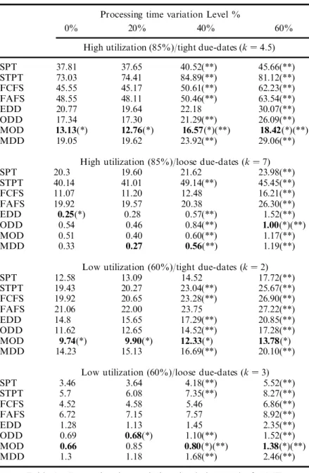
In terms of the MT measure, MOD is the best rule at the tight due-dates regard-less of the utilization and PV levels. We also note that with the loose due-dates, PV a ects the relative performance of the rules. For example, at the high utilization/ loose due dates condition (table 4), EDD gives the best MT for PV 0%, but when the level of PV increases to 60%, ODD displays better performance than EDD. Note that the di erence in the performances of ODD and EDD is statistically signi®cant (table 4). This shows that PV can create some cross-over e ects on the rules for the MT measure.

Processing time variation Level %

0% 20% 40% 60%

High utilization (85%)/tight due-dates (k 4:5)

SPT 37.81 37.65 40.52(**) 45.66(**) STPT 73.03 74.41 84.89(**) 81.12(**) FCFS 45.55 45.17 50.61(**) 62.23(**) FAFS 48.55 48.11 50.46(**) 63.54(**) EDD 20.77 19.64 22.18 30.07(**) ODD 17.34 17.30 21.29(**) 26.09(**) MOD 13.13(*) 12.76(*) 16.57(*)(**) 18.42(*)(**) MDD 19.05 19.62 23.92(**) 29.06(**)

High utilization (85%)/loose due-dates (k 7)

SPT 20.3 19.60 21.62 23.98(**) STPT 40.14 41.01 49.14(**) 45.45(**) FCFS 11.07 11.20 12.48 16.21(**) FAFS 19.92 19.57 20.38 26.30(**) EDD 0.25(*) 0.28 0.57(**) 1.52(**) ODD 0.54 0.46 0.84(**) 1.00(*)(**) MOD 0.51 0.40 0.60(**) 1.17(**) MDD 0.33 0.27 0.56(**) 1.19(**)

Low utilization (60%)/tight due-dates (k 2)

SPT 12.58 13.09 14.52 17.72(**) STPT 19.43 20.27 23.04(**) 25.67(**) FCFS 19.92 20.65 23.28(**) 26.90(**) FAFS 21.06 22.00 23.75 27.22(**) EDD 14.8 15.65 17.29(**) 20.85(**) ODD 11.62 12.65 14.52(**) 17.28(**) MOD 9.74(*) 9.90(*) 12.33(*) 13.78(*) MDD 14.23 15.13 16.69(**) 20.10(**)

Low utilization (60%)/loose due-dates (k 3)

SPT 3.46 3.64 4.18(**) 5.52(**) STPT 5.7 6.08 7.35(**) 8.27(**) FCFS 4.52 4.58 5.46 6.86(**) FAFS 6.72 7.15 7.57 8.92(**) EDD 1.28 1.13 1.45 2.35(**) ODD 0.69 0.68(*) 1.10(**) 1.52(**) MOD 0.66 0.85 0.80(*)(**) 1.38(*)(**) MDD 1.3 1.18 1.68(**) 2.46(**)

Table 4. Processing time variation simulation results for MT.

(16)

Another important point is that, up to the PV 20% level, there is little e ect on the MF or MT performance of the rules, whereas, beyond PV 40%, deterioration becomes more severe and the adverse e ect of the increasing PV is observed (®gure 4). Similar observations were also made by Yumin et al. (1994). In fact, this result came up with our previous expectation that PV has a negative e ect on the system

High Utilization (85%) / Loose due-dates (k=7)

200 220 240 260 280 300 320 340 360 380 0% 20% 40% 60%

Pr oces s ing Tim e var iation Level %

M F SPT STPT FCFS FAFS EDD ODD MOD MDD Figure 3. MF versus PV.

Low Utilization (60%) / Tight due-dates (k=2)

0 5 10 15 20 25 30 %0 %20 %40 %60 %80

Processing Time variation Level %

M T SPT STPT FCFS FAFS EDD ODD MOD MDD Figure 4. MT versus PV.

(17)

LV level % 0% 40% 80% Tight due-dates (k 2:6) SPT 186.52(*) 199.43(*)(**) 200.35(*)(**) STPT 207.72 222.66(**) 219.30(**) FCFS 223.42 244.22(**) 240.29(**) FAFS 218.63 238.43(**) 234.56(**) EDD 213.20 227.61(**) 226.40(**) ODD 205.55 224.09(**) 222.62(**) MOD 197.59 211.14(**) 208.57(**) MDD 210.86 220.66(**) 216.77(**) Loose due-dates (k 4:5) SPT 186.52(*) 199.43(*)(**) 200.35(*)(**) STPT 207.72 222.66(**) 219.30(**) FCFS 223.42 244.22(**) 240.29(**) FAFS 218.63 238.43(**) 234.56(**) EDD 211.59 225.45(**) 219.57(**) ODD 209.18 227.30(**) 226.40(**) MOD 208.31 226.37(**) 223.72(**) MDD 211.16 226.42(**) 219.21(**) Table 6. MF simulation results for Scheme 2.

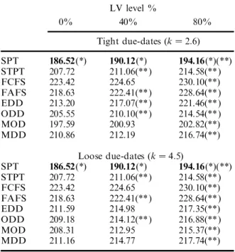
LV level % 0% 40% 80% Tight due-dates (k 2:6) SPT 186.52(*) 190.12(*) 194.16(*)(**) STPT 207.72 211.06(**) 214.58(**) FCFS 223.42 224.65 230.10(**) FAFS 218.63 222.41(**) 228.64(**) EDD 213.20 217.07(**) 221.46(**) ODD 205.55 210.10(**) 214.54(**) MOD 197.59 200.93 202.82(**) MDD 210.86 212.19 216.74(**) Loose due-dates (k 4:5) SPT 186.52(*) 190.12(*) 194.16(*)(**) STPT 207.72 211.06(**) 214.58(**) FCFS 223.42 224.65 230.10(**) FAFS 218.63 222.41(**) 228.64(**) EDD 211.59 214.98 217.35(**) ODD 209.18 214.12(**) 216.88(**) MOD 208.31 212.95 215.37(**) MDD 211.16 214.77 217.74(**)

Table 5. MF simulation results for Scheme 1.

(18)

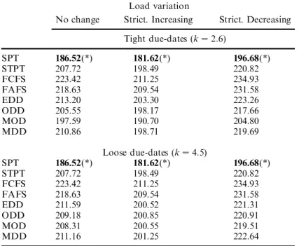
Load variation

No change Strict. Increasing Strict. Decreasing Tight due-dates (k 2:6) SPT 186.52(*) 181.62(*) 196.68(*) STPT 207.72 198.49 220.82 FCFS 223.42 211.25 234.93 FAFS 218.63 209.54 231.58 EDD 213.20 203.30 223.26 ODD 205.55 198.17 217.66 MOD 197.59 190.70 204.80 MDD 210.86 198.71 219.69 Loose due-dates (k 4:5) SPT 186.52(*) 181.62(*) 196.68(*) STPT 207.72 198.49 220.82 FCFS 223.42 211.25 234.93 FAFS 218.63 209.54 231.58 EDD 211.59 200.52 221.31 ODD 209.18 200.85 220.91 MOD 208.31 200.55 219.51 MDD 211.16 201.25 222.64

Table 7. MF simulation results for Schemes 3 and 4.

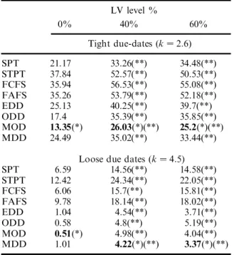
LV level % 0% 40% 60% Tight due-dates (k 2:6) SPT 21.17 24.23(**) 28.1(**) STPT 37.84 40.99 44.39(**) FCFS 35.94 38.17 43.54(**) FAFS 35.26 38.68(**) 44.67(**) EDD 25.13 28.72 33.15(**) ODD 17.4 21.63(**) 27.12(**) MOD 13.35(*) 15.97(*) 19.18(*)(**) MDD 24.49 25.92 30.49(**)

Loose Due dates (k 4:5)

SPT 6.59 7.91 10.78(**) STPT 12.42 14.4(**) 17.64(**) FCFS 6.06 7.84 10.4(**) FAFS 9.78 11.31 13.99(**) EDD 1.04 1.69(**) 2.75(**) ODD 0.58 1.26(**) 2.54(**) MOD 0.51(*) 0.95(*)(**) 2.22(*)(**) MDD 1.01 1.66(**) 3.03(**)

Table 8. MT simulation results for Scheme 1.

(19)

LV level % 0% 40% 60% Tight due-dates (k 2:6) SPT 21.17 33.26(**) 34.48(**) STPT 37.84 52.57(**) 50.53(**) FCFS 35.94 56.53(**) 55.08(**) FAFS 35.26 53.79(**) 52.18(**) EDD 25.13 40.25(**) 39.7(**) ODD 17.4 35.39(**) 35.85(**) MOD 13.35(*) 26.03(*)(**) 25.2(*)(**) MDD 24.49 35.02(**) 33.44(**)

Loose due dates (k 4:5)

SPT 6.59 14.56(**) 14.58(**) STPT 12.42 24.34(**) 22.05(**) FCFS 6.06 15.7(**) 15.81(**) FAFS 9.78 18.14(**) 18.02(**) EDD 1.04 4.54(**) 3.71(**) ODD 0.58 4.8(**) 5.19(**) MOD 0.51(*) 4.98(**) 4.04(**) MDD 1.01 4.22(*)(**) 3.37(*)(**)

Table 9. MT simulation results for Scheme 2.

Load Variation

No change Strict. Increasing Strict. Decreasing Tight due-dates (k 2:6) SPT 21.17 19.51 28.77 STPT 37.84 32.28 48.89 FCFS 35.94 30.05 45.63 FAFS 35.26 31.42 45.01 EDD 25.13 20.96 33.65 ODD 17.4 15.66 26.79 MOD 13.35(*) 11.77(*) 18.74(*) MDD 24.49 18.67 31.63

Loose due dates (k 4:5)

SPT 6.59 5.94 10.88 STPT 12.42 10.59 20.45 FCFS 6.06 5.19 10.11 FAFS 9.78 8.69 13.63 EDD 1.04 0.69 2.57 ODD 0.58 0.38(*) 2.51 MOD 0.51(*) 0.45 2.37(*) MDD 1.01 0.6 2.57

Table 10. MT simulation results for Schemes 3 and 4.

(20)

performance; however, we can provide no explicit explanation for such an e ect. Interestingly, the simple rules are robust up to an intermediate level of PV, indicating that their use would still be applicable at least to a certain extent, within the presence of such variation.

4.2. Results of load variation

The results of the simulation runs are presented in tables 5±10. As in the PV case, the results are tested for statistical signi®cance at the 95% con®dence level. Figures 5±9 are also included to support the ®ndings further.

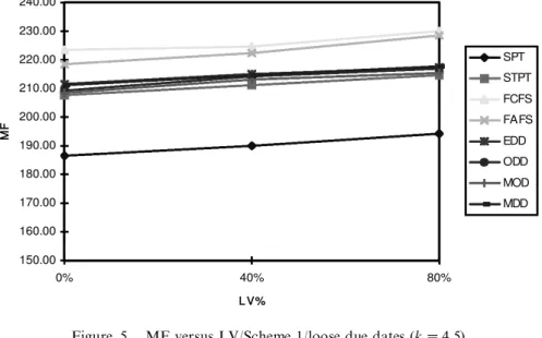
150.00 160.00 170.00 180.00 190.00 200.00 210.00 220.00 230.00 240.00 0% 40% 80% LV% M F SPT STPT FCFS FAFS EDD ODD MOD MDD

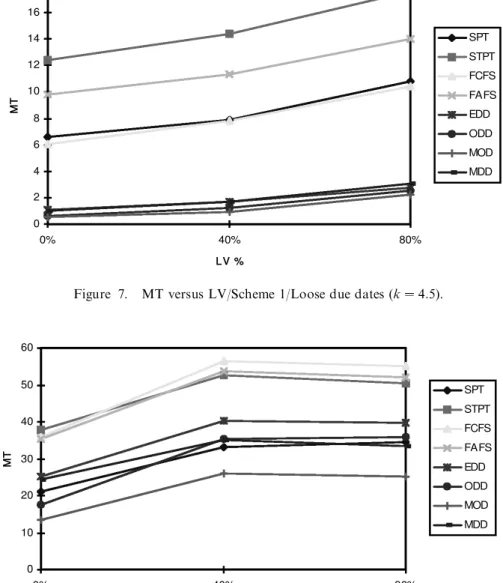
Figure 5. MF versus LV/Scheme 1/loose due dates (k 4:5).

0 5 10 15 20 25 30 35 40 45 0% 40% 80% LV % M T SPT STPT FCFS FAFS EDD ODD MOD MDD

Figure 6. MT versus LV/Scheme 1/tight due dates (k 2:6).

(21)

We have the following observations. Similar to the PV case, SPT dominates all other rules for the MF measure. This indicates that, despite the presence of LV, the relative performance of SPT with other competing rules stays una ected. The second best performance is shared by MOD with tight due dates and by STPT with loose due-dates. These two rules are followed by ODD, MDD, EDD, FAFS and FCFS. We note that the relative ranking of the rules remained the same with the LV. Among the rules, SPT seems to be the most robust rule to the changes in LV (®gure 5).

In contrast, we observe crossovers between the rules when LV is seasonal (Scheme 2) or is increasing (Scheme 3). For instance, in the seasonal LV case:

0 2 4 6 8 10 12 14 16 18 0% 40% 80% LV % M T SPT STPT FCFS FAFS EDD ODD MOD MDD

Figure 7. MT versus LV/Scheme 1/Loose due dates (k 4:5).

0 10 20 30 40 50 60 0% 40% 80% LV % M T SPT STPT FCFS FAFS EDD ODD MOD MDD

Figure 8. MT versus LV/Scheme 2/tight due dates (k 2:6).

(22)

when LV% 0%, MOD gives the best MT performanc e for loose due-dates. However, beyond the LV% 40%, MDD performs signi®cantly better than MOD and other rules. A similar crossover is observed between MOD and ODD when LV is increasing (Scheme 3). Nevertheless, apart from these exceptions, MOD yields the best MT performance.

In the case of random LV (Scheme 1), the MF and MT performances of the rules deteriorate beyond the LV% 40% level. Importantly, This e ect becomes more severe at the 80% level (®gures 5±7). However, with seasonal LV (Scheme 2), even though the performance of the rules deteriorate at the 40% level, no further deterio-ration occurs at the 80% level (®gures 8 and 9). This indicates that the performances of the rules are only sensitive to the seasonal pattern of LV change and not to the magnitude of the seasonal waves (®gure 1(b)). Another interesting observation is that the performances deteriorate signi®cantly with decreasing load level (scheme 4, tables 7 and 10), but slightly improve with increasing load level (scheme 3, tables 7 and 10). Our major conclusion is that LV negatively a ects the MF and MT performance of scheduling rules. This conclusion contradicts the results of Sabuncuoglu and Comlekci (1997) that report the robustness of rules to LV, although the latter study was done in the context of ¯ow time estimation. Nevertheless, it is crucial to note that the LV e ect is due to a combination of two factors: pattern (presented by the di erent schemes) and magnitude (controlled by LV%). The LV pattern, random, seasonal, or increasing, can only have a negative e ect. The LV magnitude, depending on the LV pattern has either neutral (seasonal) or negative (random) e ect. In summary, LV has negative e ects on the perform-ances of the rules, and the degree of the impact depends on the LV pattern and magnitude.

4.3. Results of due date variation

The rules are tested under four levels of due date variation: 20%, 40%, 60% and 80%. Two performance measures, MF and MT are used to avoid bias. To seek

0 5 10 15 20 25 0% 40% 80% LV % M T SPT STPT FCFS FAFS EDD ODD MOD MDD

Figure 9. MT versus LV/Scheme 2/loose due dates (k 4:5).

(23)

generality, two system load levels 60% and 85% as well as two due date tightness levels (Tight and Loose) are considered. In order to investigate the e ect of increas-ing the probability p of occurrence of due date changes, we consider two p levels: 0.05 and 0.10. The simulation results are illustrated in tables 11±16. The paired t-tests are applied to compare the best rule with the next best rule at a signi®cance level of 5%. The symbol (*) indicates that the di erence is signi®cant. In addition, the paired t-tests are also used to compare the original performanc e (i.e. with no due date variation) of a rule with its new performance when DV% level is increased. The symbol (**) indicates that the di erence is signi®cant.

4.3.1. Mean ¯owtime criterion

Primarily, we should mention that non due-date based rules such as SPT, STPT, FCFS and FAFS rules are insensitive to the due date variation factor. This is due to

Due date variation%

0% 20% 40% 60% 80%

High utilization (85%)/Tight due dates (k 4:5)

p 0:05 SPT 260.12* 260.12* 260.12* 260.12* 260.12* STPT 308.30 308.30 308.30 308.30 308.30 FCFS 342.15 342.15 342.15 342.15 342.15 FAFS 336.59 336.59 336.59 336.59 336.59 EDD 319.67 320.99 322.88 314.17 316.58 ODD 310.27 312.59 309.39 311.73 308.84 MOD 300.15 301.87 304.38 303.85 299.46 MDD 314.44 315.22 316.27 313.91 315.70 p 0:10 EDD 319.67 317.23 321.29 318.91 314.69 ODD 310.27 310.64 310.64 314.27 315.50 MOD 300.15 300.87 301.91 301.33 303.87 MDD 314.44 317.11 319.20 312.24 319.39

High utilization (85%)/Loose due dates (k 7)

Table 11. MF summary of results.

(24)

their primal nature that they do not consider any due date information. Consequently, as expected, these rules produce the same MF performances with all ®ve due date variation levels. We also observe that SPT always gives best MF values despite the DDV (due date variation) level, in all experimental conditions (tables 11 and 12). This indicates that DDV does not a ect the relative performance of SPT with other due-date based competing rules. Furthermore, we observe that regarding EDD, ODD, MOD and MDD, although due-date based rules, their per-formances are not a ected considerably by DDV in the high utilization case. In the low utilization case, we notice that their performances do not undergo regular de-terioration; instead, the performance of the rules ¯uctuates up and down. Nevertheless, the magnitude of up/down performance ¯uctuations is statistically insigni®cant (table 12). In summary, we conclude that the performances of priority rules are quite robust to DDV with respect to the MF measure. In addition, DDV

Due date variation%

0% 20% 40% 60% 80%

Low utilization (60%)/tight due dates (k 2)

Low utilization (60%)/loose due dates (k 3)

Table 12. MF summary of results.

(25)

does not have any signi®cant impact on the relative performance. In particular, SPT is always the best performing rule despite any DDV level.

4.3.2. Mean tardiness criterion

Analysis of due date variation for Type-I e ect. The simulation results are

tabu-lated in tables 13 and 14. As expected, non due-date based rules are insensitive to the Type-I e ect since these rules do not consider any due date information. On the other hand, due-date based rules undergo an increasing deterioration pattern along the four DDV levels. This suggests that the due date variation Type-I e ect can have a negative impact on the MT performance of the rules. As a matter of fact, the degree of this impact varies from one experimental condition to another. We observe that the slope of the deterioration curves is higher in the high machine utilization case than in the low machine utilization case. Furthermore, if we compare the rules performances in the p 0:05 case with the p 0:10 case, we observe that the

deterio-Due date variation%

0% 20% 40% 60% 80%

High utilization (85%)/tight due dates (k 4:5)

p 0:05 SPT 36.04 36.04 36.04 36.04 36.04 STPT 72.76 72.76 72.76 72.76 72.76 FCFS 45.94 45.94 45.94 45.94 45.94 FAFS 49.37 49.37 49.37 49.37 49.37 EDD 21.12 22.42 23.55 20.87 22.26 ODD 17.15 18.29 19.30(**) 21.94(**) 22.91(**) MOD 13.06* 14.49* 16.74*(**) 19.00*(**) 19.88*(**) MDD 18.38 19.86 19.63 20.77(**) 22.84(**) p 0:10 EDD 21.12 20.11 23.16 25.49(**) 24.69(**) ODD 17.15 19.08(**) 21.34(**) 28.09(**) 31.62(**) MOD 13.06* 15.08*(**) 18.98*(**) 23.13(**) 28.23(**) MDD 18.38 19.73 22.84(**) 22.98(**) 27.94(**)

High utilization (85%)/loose due dates (k 7)

p 0:05 SPT 18.83 18.83 18.83 18.83 18.83 STPT 40.09 40.09 40.09 40.09 40.09 FCFS 11.38 11.38 11.38 11.38 11.38 FAFS 20.06 20.06 20.06 20.06 20.06 EDD 0.24* 0.47(**) 1.10(**) 2.24(**) 4.46(**) ODD 0.54 0.95(**) 2.56(**) 5.65(**) 8.58(**) MOD 0.51 1.08(**) 2.92(**) 5.90(**) 7.13(**) MDD 0.30 0.48(**) 1.08(**) 2.14(**) 3.75*(**) p 0:10 EDD 0.24* 0.59(**) 1.95(**) 4.82(**) 7.36*(**) ODD 0.54 1.68(**) 4.87(**) 9.75(**) 13.84(**) MOD 0.51 1.49(**) 4.82(**) 10.29(**) 12.39(**) MDD 0.30 0.54(**) 1.77*(**) 4.59*(**) 8.40(**)

Table 13. Type I e ect/MT summary of results.

(26)

ration patterns become more severe for almost all due-date based rules. This indi-cates that the DDV Type-I e ect has a more negative impact on the performance of the rules as either the probability at which due date changes occur or the machine utilization level is increased.

Furthermore, from tables 13 and 14, we analyse the following behaviour of some rules; global rules such as MDD and EDD are more robust to Type-I e ects than local rules like ODD and MOD. This is deduced by comparing the rates at which the rules performance is deteriorated as the DDV level is increased. For instance, according to table 13, we measure the magnitude of the MT performance deterio-ration from the DV 0% to the DV 80% level. We ®nd out that the perform-ances of ODD and MOD’s performperform-ances worsen 30% in magnitude, whereas EDD and MDD’s performance s worsen by only about 10% in magnitude. This suggests that a rule which utilizes global information (i.e. job due dates) instead of local

Due date variation%

0% 20% 40% 60% 80%

Low utilization (60%)/tight due dates (k 2

p 0:05 SPT 12.60 12.60 12.60 12.60 12.60 STPT 19.24 19.24 19.24 19.24 19.24 FCFS 19.91 19.91 19.91 19.91 19.91 FAFS 21.23 21.23 21.23 21.23 21.23 EDD 14.78 15.26 14.95 15.61 15.15 ODD 11.62 12.06 12.45 12.58 13.16(**) MOD 9.74* 10.12* 10.18* 10.43* 10.77* MDD 14.28 14.97 15.22 15.48 14.85 p 0:10 EDD 14.78 14.87 15.52 15.34 15.76 ODD 11.62 12.32 13.26 13.80 13.86(**) MOD 9.74* 10.09* 10.37* 11.02* 11.55* MDD 14.28 14.94 15.02 16.13 16.24(**)

Low utilization (60%)/loose due dates (k 3)

p 0:05 SPT 3.48 3.48 3.48 3.48 3.48 STPT 5.55 5.55 5.55 5.55 5.55 FCFS 4.43 4.43 4.43 4.43 4.43 FAFS 6.84 6.84 6.84 6.84 6.84 EDD 1.26 1.36(**) 1.36(**) 1.41(**) 1.69(**) ODD 0.69 0.82(**) 1.13(**) 1.42(**) 1.79(**) MOD 0.66 0.70* 1.11(**) 1.41(**) 1.62(**) MDD 1.24 1.43(**) 1.20 1.43(**) 1.71(**) p 0:10 EDD 1.26 1.42(**) 1.50(**) 2.00(**) 2.26(**) ODD 0.69 0.91(**) 1.53(**) 1.89(**) 2.89(**) MOD 0.66 0.86(**) 1.34*(**) 1.87(**) 2.22(**) MDD 1.24 1.47(**) 1.63(**) 2.09(**) 2.19(**)

Table 14. Type I e ect/MT summary of results (continued).

(27)

information (i.e. operation due dates) is more robust to the disturbances caused by the variation in due dates.

Based on the results obtained in this section, we present a summary table (table 17) which characterizes the e ect of DDV on the priority rules for each experimental condition.

Analysis of due date variation overall e ect. The results of the simulation runs are

tabulated in tables 15 and 16. After analysing the results, we make the following observations.

Due data variation%

0% 20% 40% 60% 80%

High utilization (85%)/Tight due dates (k 4:5)

p 0:05 SPT 36.04 33.07 33.55 34.48 36.28 STPT 72.76 63.11 63.53 64.49 66.35 FCFS 45.94 44.05 45.18 47.18 50.07 FAFS 49.37 45.69 46.11 46.96 48.51 EDD 21.12 18.27 18.44 15.68 15.58 ODD 17.15 16.86 15.88 16.90 16.24 MOD 13.06* 12.46* 13.08* 12.73* 11.80* MDD 18.38 15.38 14.63 14.62 14.69 p 0:10 SPT 36.04 28.79 29.60 31.15 34.15 STPT 72.76 53.79 54.38 55.82 58.65 FCFS 45.94 42.35 44.55 48.16 52.98(**) FAFS 49.37 42.00 42.51 43.79 46.14 EDD 21.12 13.32 14.48 14.52 13.34 ODD 17.15 16.19 15.83 18.14 18.48(**) MOD 13.06* 11.43* 11.61* 11.73 12.10* MDD 18.38 12.22 12.38 11.21 13.11

High utilization (85%)/Loose due dates (k 7)

p 0:05 SPT 18.83 17.45 17.90 18.77 20.64 STPT 40.09 35.29 35.98 37.29 39.75 FCFS 11.38 11.43 12.44 14.75(**) 19.05(**) FAFS 20.06 19.22 19.50 20.18 21.86 EDD 0.24* 0.32(**) 0.40(**) 0.40(**) 0.56(**) ODD 0.54 0.56 0.55 0.55 0.74(**) MOD 0.51 0.55 0.63 0.28 0.92(**) MDD 0.30 0.28 0.34* 0.23* 0.47*(**) p 0:10 SPT 18.83 15.03 15.60 17.05 20.12 STPT 40.09 30.49 31.18 32.79 36.29 FCFS 11.38 11.33 13.33 17.62(**) 25.16(**) FAFS 20.06 18.46 18.89 20.04 22.77 EDD 0.24* 0.24* 0.27* 0.23 0.74(**) ODD 0.54 0.69(**) 0.66(**) 0.67(**) 1.10(**) MOD 0.51 0.47 0.64 0.73(**) 0.91(**) MDD 0.30 0.28 0.32 0.24 0.65*(**)

Table 15. DV overall e ect/MT summary of results.

(28)

The performances of due-date based rules, although they improve at the DV 20% level, undergo almost no change as DDV increases beyond the 40% level. This indicates that due-date based rules are quite robust to the overall e ect of DDV. Note that MOD displays the best MT performance in almost all experi-mental conditions. Even though the probability of DDV occurrence p is increased from 0.05 to 0.10, we observe no changes; due-date based rules are still una ected by DDV. In general, the relative performanc e of the priority rules is una ected by

Due date variation%

0% 20% 40% 60% 80%

Low utilization (60%)/Tight due dates (k 2)

p 0:05 SPT 12.60 11.52 11.75 12.18 12.90 STPT 19.24 16.31 16.51 16.95 17.57 FCFS 19.91 18.70 18.98 19.49 20.20 FAFS 21.23 19.01 19.08 19.32 19.78 EDD 14.78 13.18 12.53 13.08 13.06 ODD 11.62 11.30 11.56 11.75 12.08 MOD 9.74* 9.32* 9.16* 9.50* 9.97* MDD 14.28 12.27 12.54 12.87 12.07 p 0:10 SPT 12.60 10.54 10.91 11.57 12.58 STPT 19.24 14.57 14.89 15.57 16.59 FCFS 19.91 17.88 18.34 19.15 20.22 FAFS 21.23 17.39 17.54 17.95 18.71 EDD 14.78 11.00 11.02 10.70 11.39 ODD 11.62 10.84 11.40 11.92 12.29 MOD 9.74* 8.66* 8.58* 9.17* 10.06 MDD 14.28 10.20 10.39 11.15 11.20

Low utilization (60%)/Loose due dates (k 3)

p 0:05 SPT 3.48 3.19 3.31 3.64 4.57(**) STPT 5.55 4.77 5.02 5.61 6.78(**) FCFS 4.43 4.27 4.58 5.24(**) 6.57(**) FAFS 6.84 6.49 6.57 6.83 7.51 EDD 1.26 1.16 1.06 1.05 1.56(**) ODD 0.69 0.74 0.76 0.96(**) 1.24(**) MOD 0.66 0.58* 0.71 0.74* 1.16*(**) MDD 1.24 1.16 1.02 1.12 1.76(**) p 0:10 SPT 3.48 2.91 3.19 3.90 5.39(**) STPT 5.55 4.43 4.92 5.94 7.84(**) FCFS 4.43 4.25 4.81 6.02(**) 8.18(**) FAFS 6.84 6.21 6.36 6.84 8.07(**) EDD 1.26 1.00 0.99 1.35 1.98(**) ODD 0.69 0.71 0.83(**) 0.99(**) 1.99(**) MOD 0.66 0.57* 0.67* 0.91(**) 1.83*(**) MDD 1.24 1.01 0.99(**) 1.18(**) 2.02(**)

Table 16. DV Overall e ect/MT summary of results.

(29)

DDV. Nevertheless, there are some exceptions. In the high utilization/loose due dates case, we observe a crossover between EDD and MDD (table 15). At the DV 0% level, EDD displays best MT performance; however, as we get beyond the 40% level, MDD displays the best MT values and outperforms EDD. Note that the di erences between the performances of the two rules are statistically signi®cant.

5. Conclusions

In this paper, we studied the performance of well-known dispatching rules under processing time and load variations against the MF and MT measures. The main ®ndings of this study are as follows.

. Scheduling rules are not totally robust to PV. Their performances are adversely a ected by PV, especially at high PV levels (above 40%). This is consistent with the results of Sabuncuoglu and Comlekci (1997) who investigate the problem in the context of ¯ow time estimation, but in their study, only two rules are used in the simulation experiments. In our study, however, we fully focus on this issue and analyse it by using eight well-known dispatching rules. In addition, the analysis is done under various experimental conditions. Hence, our results are more conclusive. Our results do not contradict the results of Sabuncuoglu and Karabuk (1999). The former study is carried out in a static environment for a ®nite planing horizon with the emphasis on the comparisons of optimum-seeking algorithms and simple scheduling rules. The authors have found that rules are more robust to variations and random interruptions. Here, in our study, we measure the robustness of the rules in a dynamic environment for a long planning horizon (i.e. long term behaviour).

MT Performance Deterioration State Best rule Low prob. (p 0:05) High prob. (p 0:10) High utilization / MOD Moderate for local rules, Becomes more severe

tight due dates MOD and ODD.

case Less severe for global

rules, EDD and MDD.

High utilization / EDD Moderate for MOD and Becomes more severe

loose due dates ODD.

case Less severe for EDD and

MDD.

Low utilization / MOD Slightly observable Very insigni®cant

tight due dates for MOD and ODD. changes

case Almost unobservable

for EDD and MDD.

Low utilization / MOD Moderate for MOD and Becomes more severe

loose due dates ODD.

case Less severe for EDD and

MDD.

Table 17. Type-I e ect/summary of results.

(30)

. The relative ranking of the rules is only slightly a ected by PV but, in terms of MT, there are some exceptions noted for the ODD and EDD rules.

. LV, depending on its pattern and magnitude, has di erent but (at high vari-ation) negative impacts on the performances of the scheduling rules for both the MF and MT measures. However, the relative performance of scheduling rules is una ected by LV, with some exceptions for MOD, MDD and ODD in the case of the MT measure.

. The DDV Type-I e ect, de®ned as the DDV e ect due to changes in job completion times, negatively a ects the performance of due-date based priority rules. The degree of this e ect increases with the increasing probability that due dates change or as the machine utilization level increases.

. Global rules such as EDD and MDD are more robust to the DDV Type-I e ect than local rules such as ODD and MOD.

. The MT performance of due-date based rules, although negatively a ected by the Type-I e ect, is quite robust to the overall e ect of DDV. This indicates that the e ect of DDV due to changes in completion times (Type-I e ect), is eventually neutralized by the DDV e ect due to changes in due dates (Type-II e ect).

. The relative performances of priority rules are, in general, una ected by the overall e ect of DDV. However, there are still some exceptions that we noted for the rules EDD and MDD.

. In almost all experimental conditions, MOD gives the best MT values irre-spective of the level of DDV. This con®rms the results of previous studies for job shops. Furthermore, this makes us more con®dent in suggesting MOD as an e ective rule for MT, even in job shop environments where variation in due dates can occur.

In conclusion, PV, LV and DDV do not much threaten the relative performance of the competing rules, even though they have an intense negative e ect on their individual performances at high variation levels. Although the robustness of the relative performance of the rules to PV/LV/DDV provides a worthy relief to practi-tioners in the ®eld, we suggest that PV/LV/DDV should not be ignored in the sched-uling studies, barring that they may cause irreparable de®ciencies to the whole job shop system performance. There is a need to develop new rules or scheduling mechanisms that are quite robust to variations in real production environments.

References

Baker, K. R., 1984, Sequencing rules and due date assignments in a job shop. Management

Science, 30(9), 1093±1104.

Baker, C. T. and Dzielinski, B. P., 1960, Simulation of a simpli®ed job shop. Management

Science, 6(3), 311±323.

Carroll, D. C., 1965, Heuristic sequencing of single and multiple component jobs. PhD dissertation, MIT.

Conway, R. W., 1964, An experimental investigation of priority assignment in job shop.

RAND Corp. Memo. RM-3789-PR (February).

Eilon, S. and Chowdhury, I. G., 1976, Due dates for job shop scheduling. International

Journal of Production Research, 14, 223±237.

Elvers, D. A. and Taube, L. R., 1983, Time completion of various dispatching rules in job shops. Omega, 11(1), 81±89.

(31)

Elvers, D. A., 1973, Job shop scheduling rules using various delivery due date setting criteria.

Prod. Inv. Mgmt, 14(4), 62±70.

Frostig, E., 1988, A stochastic scheduling problem with intree precedence constraints.

Operations Research, 36(6), 937±943.

Hottenstein, M. P., 1970, Expediting in job-order-control systems: a simulation study. AIIE

Transactions, 6, 302.

Jones, C. H., 1973, An economic evaluation of job shop dispatching rules: a clarifying analy-sis. Management Science, 28(11), 1337±1341.

Law, A. M. and Kelton, W. D., 1991, Simulation Modeling and Analysis (McGraw-Hill). Lawrence, S. R. and Sewell, E. C., 1997, Heuristic, optimal, static, and dynamic schedules

when processing times are uncertain. Journal of Operations Management, 15, 71±82. Pegden, C. D., Shannon, R. E. and Sadowsky, R. P., 1995, Introduction to Simulation

Using Siman (McGraw-Hill).

Pinedo, M., 1982, Minimizing the expected makespan in stochastic ¯ow shops. Operations

Research, 30(1), 148±162.

Pinedo, M., 1995, Scheduling: Theory, Algorithms and Systems (Prentice-Hall).

Pinedo, M. and Weiss, G., 1987, The `largest variance ®rst’ policy in some stochastic sched-uling problems. Operations Research, 35(6), 884±891.

Ramasesh, R., 1990, Dynamic job shop scheduling: a survey of simulation research.

International Journal of Management Science, 18(1), 43±57.

Sabuncuoglu, I. and Comlekci, A., 1997, Flowtime estimation in dynamic job shops.

Research Report: IEOR±9714, Department of Industrial Engineering, Bilkent University.

Sabuncuoglu, I. and Karabuk, S., 1999, Rescheduling frequency in an FMS with uncertain processing times and unreliable machines. Journal of Manufacturing Systems, 18(4), 1± 16.

Smith, M. L., Panwalker, S. S. and Dudek, R. A., 1973, Scheduling with uncertain pro-cessing times. 44th ORSA Meeting, San Diego, CA.

Suresh, S., Foley, R. D. and Dickey, S. E., 1985, On Pinedo’s conjecture for scheduling in a stochastic ¯ow shop. Operations Research, 33(5), 1146±1153.

Vepsalainen, A. P. J. and Morton, T. E., 1987, Priority rules for job shops with weighted tardiness costs. Management Science, 33(8), 1035±1047.

Weeks, J. K. and Fryer, J. S., 1977, A methodology for assigning minimum cost due dates.

Management Science, 23(8), 872±881.

Yumin, H., Smith, M. L. and Dudek, R. A., 1994, E ects of inaccuracy of processing time estimation on e ectiveness of dispatching rules. Institute of Industrial Engineers, 3rd

Industrial Engineering Research Conference Proceedings. Hyatt Regency Atlanta,

Atlanta, Georgia, 18±19 May.