a thesis
submitted to the department of electrical and
electronics engineering
and the institute of engineering and science
of bilkent university
in partial fulfillment of the requirements
for the degree of
master of science
By
Refik C
¸ a˘glar KIZILIRMAK
August, 2006
Prof. Dr. Hayrettin K¨oymen (Supervisor)
I certify that I have read this thesis and that in my opinion it is fully adequate, in scope and in quality, as a thesis for the degree of Master of Science.
Asst. Prof. Dr. Defne Akta¸s
I certify that I have read this thesis and that in my opinion it is fully adequate, in scope and in quality, as a thesis for the degree of Master of Science.
Dr. Satılmı¸s Topcu
Approved for the Institute of Engineering and Science:
Prof. Dr. Mehmet B. Baray
Director of the Institute Engineering and Science ii
OPTIMIZATION IN ISTANBUL
Refik C¸ a˘glar KIZILIRMAK
M.S. in Electrical and Electronics Engineering Supervisor: Prof. Dr. Hayrettin K¨oymen
August, 2006
The aim of this work is to design a complete PMR (Professional Mobile Ra-dio) network based on CDMA 450 in Istanbul metropolitan region. Coverage and capacity analysis are performed by the developed simulation software tool. Trade off between several system parameters such as quality of service, user mo-bility, traffic distribution, data rate and bandwidth are considered to optimize the capacity and coverage of the network. Since, managing system interference by precise power control is a very critical concept for CDMA; forward and re-verse link interference analysis, and their effects are also studied. Coverage and handoff areas are shown on the map by the aid of GIS (Geographical Information Systems) tool. System capacity and coverage are presented as the main results of the proposed network.
Keywords: CDMA 450, Cell Design, Network Optimization, PMR. iii
˙ISTANBUL’DA CDMA-PMR A ˘G PLANLAMASI VE
OPT˙IM˙IZASYONU
Refik C¸ a˘glar KIZILIRMAK
Elektrik ve Elektronik M¨uhendisli˘gi, Y¨uksek Lisans Tez Y¨oneticisi: Prof. Dr. Hayrettin K¨oymen
A˘gustos, 2006
Bu tezde ama¸c, ˙Istanbul’da bir CDMA 450 tabanlı PMR (Private Mobile Radio) a˘gı tasarlamaktır. Kapasite ve kapsama analizleri geli¸stirilen bilgisayar programı yardımı ile yapılmı¸stır. Bant geni¸sli˘gi, veri hızı, kullanıcı hareketlili˘gi, trafik da˘gılımı gibi sistem parametreleri arasındaki ili¸skiler, bu a˘gın kapasitesini ve kap-samasını optimize etmek i¸cin kullanılmı¸stır. CDMA’de hassas bir g¨u¸c kontrol¨u yapmak, sistem enterferansını kontrol etmek a¸cısından ¸cok ¨onemli oldu˘gundan, ileri ve geri ba˘glantıdaki enterferans hesaplamaları ve etkileri ayrıca g¨osterilmi¸stir. Kapsama ve h¨ucre de˘gi¸sim alanları CBS (Co˘grafi Bilgi Sistemi) yardımı ile harita ¨uzerinde g¨osterilmi¸stir. Tasarlanan sistemin kapsama alanı ve kapasitesi sonu¸c olarak sunulmu¸stur.
Anahtar s¨ozc¨ukler : CDMA 450, H¨ucre Tasarımı, A˘g Optimizasyonu, PMR. iv
I would like to express my gratitude to my supervisor Prof. Dr. Hayrettin K¨oymen for his instructive comments in the supervision of the thesis.
I would like to thank all the former and present members of Communica-tions and Spectrum Management Research Center (˙ISYAM) for their support and close working relationships, especially Deputy Director Dr. Satılmı¸s Topcu and Director Prof. Dr. Ayhan Altınta¸s.
I would like to express my special thanks and gratitude to Asst. Prof. Dr. Defne Akta¸s and Dr. Satılmı¸s Topcu for showing keen interest to the subject matter and accepting to read and review the thesis.
Finally, I would like to express my thanks to my family for their trust, en-couragement and support throughout my life.
1 Introduction 1
1.1 CDMA System Overview . . . 1
1.1.1 Evolution of 3G Technology . . . 4
1.2 Basics of CDMA . . . 5
1.2.1 Power Control . . . 6
1.2.2 Capacity . . . 9
1.2.3 Forward and Reverse Link Structures . . . 14
1.3 PMR Overview . . . 15
1.3.1 What is CDMA 450? . . . 17
1.4 Objectives and Organization . . . 18
2 Modeling and Optimization 20 2.1 Simulation Tools and Methods . . . 20
2.2 CDMA Network Modeling . . . 22
2.2.1 Capacity and Coverage Planning . . . 22
2.3 Cell Design Algorithm . . . 28
2.3.1 Evaluation of Cell Design Algorithm . . . 31
3 Design of a CDMA-PMR network in Istanbul 34
4 Conclusions 45 4.1 Discussions . . . 45 4.2 Future Work . . . 51 Appendices 55 A List of Acronyms 56 B Software Tool 57
1.1 Upgrade paths from 2G to 3G. . . 5 1.2 In CDMA, each users’ transmit power is assigned by power control
to achieve the same received power Pr at base station. . . 7
1.3 All signals from base station fade together to the same power level
when they arrive to the mobile. . . 8
1.4 Mobiles of neighboring cells also affect the interference at the base
station. . . 11
1.5 Pole capacity decreases as other-cell interference factor f increases. 12
1.6 Base Station sensitivity decreases as number of mobiles increases. 13
1.7 Noise rise approaches infinity as cell loading approaches 1. . . 14
1.8 Forward link channels. . . 15
1.9 Spectrum usage of cdma450 at subclass A. . . 18
2.1 Coverage of the base station C¸ amlıca changes due to the active
number mobiles in that cell. The number of active mobiles are 48 and 1 in (a) and (b). The blue region contour shows the region in which both forward and reverse links have reliable communication. Also, users are assumed to be uniformly distributed in that region. 21
2.2 CDMA network design process. . . 22
2.3 Path losses ,LXY, are calculated at each grid point(X,Y) for each
base station. . . 23
2.4 A mobile receives 3 signals from 3 base stations, signal from BS1
is taken as the desired signal, and other signals are as interferers. 24
2.5 Sample Forward Link analysis. Grid points are tested for required
Eb/Nt and area formed by succeeded points is the forward link
coverage area. . . 27
2.6 Flow diagram of iteration steps. Mk(i), fk(i) and ρk(i) indicate the
number of mobiles, other-cell interference factor and cell loading
in cell i at iteration k. . . . 29
2.7 Calculating interference from other cell’s mobiles. . . 31
2.8 Behavior of two adjacent cells with different cell loadings and
other-cell interference effects. . . 32
3.1 Traffic distribution of the existing PMR network and transmitter
locations on map. . . 35
3.2 Horizontal pattern of the antennas used in the network. . . 37
3.3 Other-cell interference factors, cell loadings, number of users and
noise rises in each cell in the network. . . 41
3.4 Coverage areas of each cell in the network. Cell loadings are 80%
in each cell. . . 43
4.1 In the rectangle, generated traffic by one of the existing PMR networks is 3.83 Erlang and capacity of proposed network is 87.74
Erlang. . . 46
4.2 Coverage areas of each cell in the network. Cell loadings are 100%
for cell S¸i¸sli and 80% for all others. . . 47
4.3 Coverage areas of each cell in the network. Cell loadings are 100%
in each cell. . . 49
4.4 Handoff regions for approximately 35% loading in each cell. . . 50
B.1 Sample parameters windows of simulator. . . 59
1.1 Frequency bands for cdma2000 . . . 5
1.2 450 MHz Band Subclasses . . . 17
2.1 Required Eb/Nt on the downlink as a function of mobile speed . . 26
3.1 List of base stations . . . 36
3.2 Converged results for the CDMA-PMR network . . . 42
Introduction
Mobile and wireless communications have become an integral part of cations networks. With increase in demand for high data rate and new communi-cations services, we will continue to see the rapid growth in popularity of wireless communications systems. Code Division Multiple Access (CDMA) based next generation communications systems promise significant higher data rates and va-riety of applications such as video teleconferencing and Internet applications.
In 1978, a CDMA system had been proposed [1]. However the interest was not high until the Qualcomm demonstrated the implementation of such a system in the late 1980’s. Since then, CDMA has become a very attractive technique for wireless communications. Research on this subject mainly concentrates on design of receivers, coding and modulation techniques and power control algorithms. Work in network design and optimization also receive attention [2, 3, 4].
1.1
CDMA System Overview
Code Division Multiple Access (CDMA) is basically a spread spectrum multi-ple access scheme. CDMA provides some unique features such as high spectrum efficiency, low transmit power, robust handoff procedures [5, 6]. These features
make CDMA advantageous over other multiple access schemes like TDMA (Time Division Multiple Access) and FDMA (Frequency Division Multiple Access). The two common techniques used for spread spectrum communications are direct se-quence (DS) modulation and frequency hopping (FH). In DS modulation, the data is spread by directly multiplying it with much faster pseudo-noise code se-quence. In FH, the carrier frequency is ’hopping’ according to a unique sese-quence. In this research, focus will be on DS modulation only.
In CDMA, each user’s signal is multiplied by a high rate pseudo-random code sequence in order to convert their narrowband signal to wideband signal. All users in a CDMA system share the same frequency spectrum. Therefore, if user’s signals in CDMA system are considered in time or frequency domain only, the signals appear to be overlapping, but they distinguish each other by their special codes. In the receivers, the signals are correlated by the appropriate pseudo-random code which despreads the spectrum. The other user’s signals whose codes do not match are not despread and therefore appear as noise and introduce interference to the system. In CDMA, signal to interference (SIR) ratio is determined by the ratio of desired signal power to the total interference power from all other users. This is the only limitation in capacity of CDMA system and that is the reason why CDMA is interference limited. On the other hand, TDMA and FDMA are mainly bandwidth limited.
A CDMA system must be optimized from a system point of view, so that the system can tolerate maximum interference level [2]. Number of users that can be supported in CDMA system is a measure of capacity of that system. The capacity enhancement can be achieved by properly managing the transmitters’ power levels. In other words, the precise power control is very critical concept for CDMA technology. There are numerous proposed power control algorithms [7, 8, 9, 10, 11, 12]. Most of them are developed to solve the near-far problem. Consider a base station and two mobiles (one close to base station, other far away). If both mobiles’ transmit powers were the same, base station would receive more power from the nearer mobile. Since one transmission is the other’s interference, the SIR of the far away mobile will be much lower. The problem can be solved if the closer mobile use less power so that the SIR for all transmitters at the base
station is roughly the same.
As mentioned, CDMA cellular systems are interference limited systems in which link performance depends on the ability to detect the desired signal in the presence of interference. In such system, any technique that reduces multiple access interference translates into a capacity gain. CDMA systems use speech coding techniques in order to transmit speech with the highest possible quality using the least possible channel capacity. This can be accomplished by decreasing the rate of speech coders when silent period detected in speech waveform. Voice activity detection is counted as one of the capacity enhancement techniques in a CDMA system.
Cell sectoring is another powerful technique for increasing the capacity of a CDMA system as in other cellular systems [13, 14].
In cellular networks, as a mobile moves from the coverage area of one base station (source cell) to the coverage area of another base station (target cell), a handoff must occur to transfer the communication link from one base station to another base station. There are different handoff processes; soft handoff, softer handoff and hard handoff. The process is called soft handoff if mobile is connected to both cells until the connection is well established in the target cell. If the soft handoff occurs between the two sectors of the same cell, it is called softer handoff. Unlike the soft handoff, as mobile moves from one cell to another, if it drops its existing connection and then establishes a new connection, the process is called hard handoff which is used in TDMA and FDMA systems. In CDMA systems, the term hard handoff is used to indicate the transitions between two different CDMA carriers.
It is difficult to implement hard handoff as in TDMA and FDMA systems in power controlled CDMA systems because a system with power control attempts to dynamically adjust transmitter power while in operation. For power control to work properly, the mobile must be linked at all times to the base station from which it receives the strongest signal. Soft handoff can guarantee the mobiles are linked at all time whereas the hard handoff can not. Power control is closely related to soft handoff. CDMA uses both power control and soft handoff as an
interference reduction mechanism [13, 15].
A CDMA system can support different number of users in reverse (MS to BS) and forward links (BS to MS). The capacity of a CDMA system depends on the reverse link capacity which is generally said to be less than the forward link capacity [3, 16, 17, 18, 19]. The forward link capacity is set by total transmitted power at base station and its distribution between the channels including pilot, traffic, synchronization and paging channels. If the power on traffic channels is not enough, the system becomes forward link limited.
1.1.1
Evolution of 3G Technology
CDMA technology is first commercially marketed by Qualcomm Inc. and stan-dardized as IS-95A in 1995 [20]. This new technology, also called cdmaOne, appeared in the market at the same time of GSM as a 2G system. Initially, both GSM and cdmaOne could offer data rates up to 14.4 kbps. Since then, they have followed different paths to 3G. GSM first upgraded to GPRS (General Packet Radio Service) with data rate of 115 kbps. Then, EDGE (Enhanced Data Rate for GSM Evolution) was built on GPRS and allowed GSM operators to use their existing networks to offer IP-based services and applications at the speed of 384 kbps. EDGE technology was the last step for GSM before 3G W-CDMA. On the other hand, to reach higher data rates, IS-95A first upgraded to IS-95B (115 kbps) and then to cdma2000 1X. At this step, the capacity of IS-95A is doubled and data rates were close to 3G data speed. While the speeds were increasing, the name 3G began to be expressed in the market and ITU (International Telecommunication Union) identified the 3G standards in the name of IMT-2000 which includes the spectrum usage and technical standards. In Europe, W-CDMA which is devel-oped by ETSI (European Telecommunications Standards Institute) was accepted as a 3G standard by IMT-2000. In 2000, all developing W-CDMA technologies integrated in the same name of UMTS. On the other hand, in North America cdma2000 also satisfied the requirements and became another standard for 3G. In addition to W-CDMA and cdma2000, there are other IMT-2000 standards which are Chinese TDMA/CDMA based TD-SCDMA, TDMA based UWC-136
and FDMA based DEC. The upgrade paths to most common 3G technologies are shown in Figure 1.1.
Figure 1.1: Upgrade paths from 2G to 3G.
Suggested frequency bands for cdma2000 are given in Table 1.1. Currently, cdma2000 is commercially available and is being deployed mostly in the 450 MHz frequency band.
Table 1.1: Frequency bands for cdma2000
Band Reverse Link Forward Link
1 450MHz 450 - 457.5 460 - 467.5
2 800MHz 824 - 849 869 - 894
3 1900MHz 1850 - 1910 1930 - 1990
4 2100MHz 1920 - 1980 2110 - 2170
1.2
Basics of CDMA
This section presents the basic characteristics of a CDMA network which have direct effects on the network performance.
1.2.1
Power Control
In CDMA, since all mobiles transmit at the same frequency, the internal inter-ference of the network plays a critical role in determining the capacity of the network. The transmit powers of each mobile must be controlled to limit the interference.
Power control is basically needed to solve near-far problem. In order to reduce the near-far problem, the main idea is to achieve same received power level from all mobiles at the base station. Each received power should be at the minimum
level that still allows the link to meet the system requirements such as Eb/N0. In
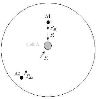
order to receive the same power level at the base station, the mobiles that are closer to the base station should transmit less power than the mobiles far from the base station. In Figure 1.2, there are two mobiles of the cell A, A1 which is closer
to the base station and A2 which is far from the base station. Pr is the minimum
signal level for required system performance. Therefore, the mobile A2 should
transmit more power than A1 to achieve same Pr at the base station, PA2>PA1.
If there was no power control, in other words their transmit power were the same, the received signal from A1 would be much larger than A2. Therefore, S/I would be low for A2 and A1 would not allow A2 to have a reliable communication since they share the same spectrum band.
1.2.1.1 Reverse Link Power Control
Beside the near far effect described above, the immediate problem is to determine the mobile’s transmit power when it first establishes a connection. Before the mobile has contact with the base station, it has no idea about the amount of interference in the system. Therefore, the mobile is in suspense about its initial transmit power. If the mobile attempts to transmit high power to guarantee the contact, it may introduce too much interference. On the other hand, if mobile transmits at lower power not to disturb other mobiles’ connections, its power may
not meet the required Eb/N0. As specified in IS-95 standards, the mobile acts
Figure 1.2: In CDMA, each users’ transmit power is assigned by power control
to achieve the same received power Pr at base station.
probe with low power. The mobile sends its first access probe, and then it waits for a response from base station for a time, if it does not receive any response, then second access probe is sent with higher power. The process is repeated until the base station responds. If the responded signal by base station is high, mobile understands that base station is closer and enters the network with low transmit power. Likewise, if the responded signal is low, mobile knows the path loss is large and transmits high power. In this operation, base station does not tell mobile its transmit power, but mobile estimates its own transmit power.
The process described above is called open loop power control since it is con-trolled by only mobile itself. Open loop power control starts when mobile first attempts to communicate with base station and continues during the connection. This power control is used to compensate for the slow varying shadowing effects. However, since the reverse and forward links are on different frequencies, estimat-ing the transmit power due to the forward path loss of base station will not give the precise solution to power control. This power control will fail or be too slow for fast Rayleigh fading channels.
The closed loop power control is used to compensate for the fast Rayleigh fading. This time, mobile’s transmit power is controlled by the base station. For this purpose, base station continuously monitors the reverse link signal quality and if the link quality is bad, it tells the mobile to power up, similarly if the link quality is very high, the base station command the mobile to power down.
1.2.1.2 Forward Link Power Control
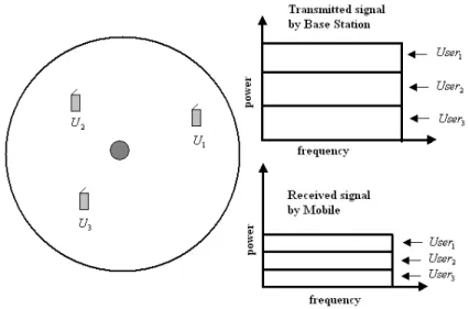
Similar to reverse link power control, forward link power control is also needed to keep the forward link quality at a specified level. This time, mobile monitors the forward link quality and tells base station to power up or power down. This power control has no effect on near-far problem, since all signals fade together to the same power level when they arrive to the mobile. Briefly, there is no near-far problem in forward link. Figure 1.3 illustrates this.
Figure 1.3: All signals from base station fade together to the same power level when they arrive to the mobile.
1.2.2
Capacity
In essence, the capacity of a CDMA network is interference limited. Maximum number of mobiles that can be supported by the network is called pole capacity and this quantity is the basic measure of capacity of a CDMA network. In order to formulate the capacity, the amount of interference introduced by the system users need to be determined. Following calculations are given for reverse link which is the limiting direction.
In digital communications, the metric Eb/Nt, or energy per bit per noise power
density, is primarily used in link calculations. Here, the term Nt indicates the
total interference power density due to other mobiles plus thermal noise power density.
If S is the signal power and R is the data rate, the bit energy Eb is,
Eb =
S
R (1.1)
In reverse link, because of the power control, all mobiles reach at the base station
with same power of S, the Nt is
Nt= I0+ N0 =
(M − 1)vfS
W + N0 (1.2)
where M is the number of mobiles, W is the bandwidth and vf is voice activity
factor.
Eb/Nt becomes, Equation 1.1 divided by Equation 1.2;
Eb Nt = (W R) S N0W + (M − 1)vfS (1.3)
Equation 1.3 relates the energy per bit (Eb/Nt) to two factors; the signal to
intererence ratio S/N of the link and the ratio of transmitted bandwidth W to bit rate R. The ratio W/R is also known as the processing gain of the system,
Gp. Solving Equation 1.3 for M we get;
M = 1 + Gp 1 (Eb/Nt)vf − N0W Svf (1.4)
As seen in Equation 1.4, maximum number of mobiles can be reached as S goes to infinity. This is theoretical limit and can not be reached in real life since transmit
powers of mobiles are limited. This asymptotic cell capacity Mmax is called pole
capacity and given in Equation 1.5.
Mmax = 1 + Gp
1 (Eb/Nt)vf
(1.5)
We can add imperfect power control effect as a coefficient ηp. For instance if it
is 0.85, that means approximately 15 percent of its capacity is lost due to the imperfect power control. Equation 1.5 becomes;
Mmax = 1 + Gp
ηp
(Eb/Nt)vf
(1.6)
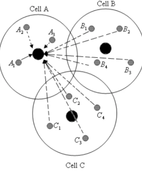
Equation 1.6 is given for a single cell network, however in an actual multi-cell CDMA network, the mobiles in neighboring cells also introduce interference and this interference can not be power controlled since those mobiles are controlled by their own base stations. Figure 1.4 shows the effect of other cells’ mobiles. Total number of other-cell mobiles is generally much larger than the number of own cell mobiles. However, their average received power at the base station is said to be some fraction (f) of own cell received power. Therefore, total interference can
be written as Svf(M-1)(1+f). Equations 1.4 and 1.6 can be modified to include
the other cell effect as,
M = 1 + Gp ηp (Eb/Nt)vf(1 + f ) − N0W ηp Svf(1 + f ) (1.7) Mmax = 1 + Gp ηp (Eb/Nt)vf(1 + f ) (1.8) where,
f : other-cell interference factor;
f = Pother Pincell
Figure 1.4: Mobiles of neighboring cells also affect the interference at the base station.
Pother: Total other cell received power
Pincell : Total own cell received power
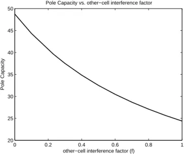
f is a very critical parameter to obtain the maximum number of mobiles in
a cell. For a single cell system, f is zero and if the required Eb/Nt is 6.5 dB
and processing gain is 128 (bandwidth is 1.23 MHz, data rate is 9.6 kbps), if we neglect 1, the Equation 1.8 returns 48 users for voice activity of 0.5 and imperfect power control coefficient of 0.85.
However, for multi-cell networks, f would not be zero and Figure 1.5 shows how the pole capacity changes with respect to interference factor f.
Also, if we solve Equation 1.7 for S, we would find the minimum required
received power by the base station to satisfy the given Eb/Nt for a given number
0 0.2 0.4 0.6 0.8 1 20 25 30 35 40 45 50
other−cell interference factor (f)
Pole Capacity
Pole Capacity vs. other−cell interference factor
Figure 1.5: Pole capacity decreases as other-cell interference factor f increases.
S = (Eb/Nt)N0 1 R − (M −1)vf(1+f )(Eb/Nt) W ηp (1.10)
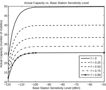
This S value is the base station sensitivity, so any mobile who wants to have a reliable communication should exceed this value to tolerate other mobiles’ in-terference. Figure 1.6 shows the relationship between sensitivity and number of mobiles for different f values. This also explains the dependence of cell size on number of mobiles and other-cell interference factor. Also in Figure 1.6, note that as received power S increases, system reaches its pole capacity.
In addition to other-cell interference factor f, there are other parameters like cell loading and noise rise to evaluate the system performance.
Cell loading, ρ, is the ratio of actual capacity to the pole capacity, M/Mmax.
If we divide Equation 1.7 by Equation 1.8, we get ρ;
ρ = M Mmax = M M + N0W ηp Svf(1+f ) = Svf(1 + f )M N0W + Svf(1 + f )M (1.11)
−12010 −110 −100 −90 −80 −70 −60 −50 15 20 25 30 35 40 45 50
Actual Capacity vs. Base Station Sensitivity Level
Base Station Sensitivity Level (dBm)
Actual Capacity (number of mobiles)
f = 0 f = 0.25 f = 0.50 f = 0.75 f = 0.99
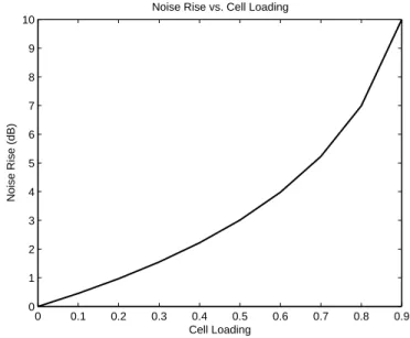
Figure 1.6: Base Station sensitivity decreases as number of mobiles increases. noise level; ηr = N0W + Svf(1 + f )M N0W = 1 1 − ρ (1.12)
Note that when ρ approaches 1, ηrapproaches infinity and the system reaches
its pole capacity. Figure 1.7 illustrates the relationship between ρ and ηr.
Cell loading and noise rise concepts can be easily related to the cell size. As stated before, S is the received signal power from one mobile by the base station. If S is very high, cell loading approaches 100%. S is high when mobiles are very close to the base station, in other words when the cell size is small. Similarly, if
the received powers from mobiles are as low as the thermal noise level, ηr is very
small and cell loading is close to zero percent. In that case, cell size would be very large.
0 0.1 0.2 0.3 0.4 0.5 0.6 0.7 0.8 0.9 0 1 2 3 4 5 6 7 8 9 10
Noise Rise vs. Cell Loading
Cell Loading
Noise Rise (dB)
Figure 1.7: Noise rise approaches infinity as cell loading approaches 1.
1.2.3
Forward and Reverse Link Structures
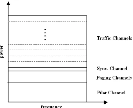
IS-95 based CDMA networks have different link structures in forward and reverse links. The forward link consists of four different channels; pilot, synchronization, traffic and paging channels. There is one pilot channel, one synchronization channel, seven paging channels and several traffic channels. Each of these forward link channels is spread orthogonally to form a composite spread spectrum signal to be transmitted by the base station. In Figure 1.8, the power ratios allocated to these different channels are shown.
Ppilot = 15%-20%Ptotal
Psync = 1.5%-2%Ptotal
Ppaging = 7%Ptotal
Ptraf f ic = 71%-76%Ptotal
Ptraf f ic/mobile = Ptraf f ic / total number of mobiles
traffic channel. There is no need to transmit a pilot signal from the mobile.
Figure 1.8: Forward link channels.
1.3
PMR Overview
Professional or Private Mobile Radio (PMR) is a radio network which is operated by wide range of professional organizations to support their own activities. Police and fire services, the utilities (Gas, Water, Electricity), transportation companies, factories and airports are just some of the many organizations which are using PMR.
Some of the features that are specific to PMR are; • Push-to-talk voice services
• One-to-many/Group calls • Packet data
• Fast call set-up
• Automatic and priority call queuing when system busy • Closed user groups
• Simultaneous voice and data transfer
• Ability to directly interconnect with other public networks
The existing PMR market in Europe is generally based on analog technologies with 97 % analog users in the year 2000. In 2001 around 60 % of new users, the majority being public safety and security applications chose digital technologies [21]. Although analog technology will still be in use, it is expected that within 4-5 years the majority of the PMR market will upgrade to new digital technologies.
In parallel to the developments in digital land mobile technology, the demand for applications based on high speed data is increased. Already now, these de-mands are expressed in PMR market, where the traditional narrow band analog technology is insufficient. In response, industry has already developed a number of systems, including for example TETRA TAPS using 200 kHz channel band-width and CDMA-PMR using 1.25 MHz channel bandband-width.
In [21, 22, 23, 24, 25, 26], CDMA-PMR is investigated in terms of its spectrum efficiency, potential frequency bands and adjacent band compatibility between existing narrow band PMR systems. In [22] the CDMA-PMR system is proposed for frequencies around 410-430 MHz and 450-470 MHz bands and in [16, 25] it is concluded that spectrum efficiency (capacity/spectrum bandwidth) for CDMA-PMR is found significantly higher than for TETRA and for GSM.
1.3.1
What is CDMA 450?
More than 40 countries around the world use 450 MHz band for the first gener-ation analog Nordic Mobile Telephone (NMT) networks. Most NMT operators have narrow band allocation and can not supply the demand for high speed data applications. As a result, to attract subscribers, NMT operators need to upgrade their networks to 3G while still operating at 450 MHz. For this purpose, manu-facturers developed a technology called CDMA 450 which is basically cdma2000 operating at 450 MHz frequency band.
In the market, CDMA 450 is a very significant contender with its wide area coverage and all advantages of 3G technology such as higher data rate, push-to-talk and location-based services etc. Presently these systems are not allowed to be used in Turkey, because the regulatory authority did not yet assigned frequency bands for their operation. However it is expected that this will soon be possible.
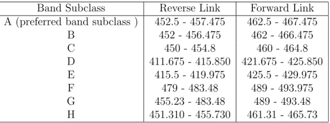
Suggested band subclasses for CDMA 450 are given in Table 1.2. Table 1.2: 450 MHz Band Subclasses
Band Subclass Reverse Link Forward Link
A (preferred band subclass ) 452.5 - 457.475 462.5 - 467.475
B 452 - 456.475 462 - 466.475 C 450 - 454.8 460 - 464.8 D 411.675 - 415.850 421.675 - 425.850 E 415.5 - 419.975 425.5 - 429.975 F 479 - 483.48 489 - 493.975 G 455.23 - 483.48 489 - 493.48 H 451.310 - 455.730 461.31 - 465.73
Most of the countries use the subclass A for NMT networks. In Turkey, this subclass A band is allocated not for NMT, but for PMR. Therefore, these PMR operators can upgrade their networks to CDMA 450 while still using the same frequency band. In Turkey, subclass E is used for NMT networks.
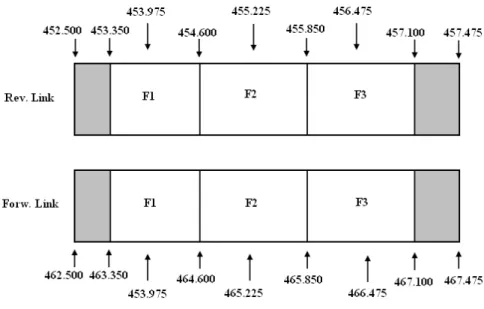
Detailed spectrum of CDMA 450 service at subclass A is given in Figure 1.9. There are three different carrier frequencies with a bandwidth of 1.25 MHz and
guard bands at the beginning and end of the frequency band.
Figure 1.9: Spectrum usage of cdma450 at subclass A.
1.4
Objectives and Organization
The aim of this work is to design a PMR network based on CDMA 450 in ˙Istanbul metropolitan region. For this purpose, a cell design algorithm and a software tool that implements this algorithm are developed. This tool is used to perform detailed capacity analysis and obtain coverage areas of the proposed CDMA 450 network.
Organization of this thesis is as follows: Chapter 2 explains the both forward and reverse link calculations and also introduces an iterative cell design algorithm. In Chapter 3, design process of a complete CDMA-PMR network in Istanbul is given and performance of the network is discussed. Finally, the thesis is concluded with discussions and future works in Chapter 4.
the amount of other-cell interferences for each cell in the proposed CDMA-PMR network is given in detail.
Modeling and Optimization
2.1
Simulation Tools and Methods
Design of any reliable radio network needs a computer aided GIS based simulation tool [27]. For this purpose, ˙ISYAM has developed software called BILSPECT which offers a set of applications including propagation prediction, analog/digital broadcasting analysis, land mobile analysis etc. The correctness of all of these network simulation results are related to propagation and coverage prediction which relies on the correctness of the propagation model and digital elevation data. BILSPECT can perform propagation simulations with a number of models proposed by ITU (International Telecommunications Union). Also, integrated GIS tool enables the coverage areas to be mapped and helps to analyze the situation in detail.
In case of CDMA network simulation, as compared to other cellular networks, it is considerably more complex. One of the fundamental characteristics of CDMA systems is that the coverage area is directly related to the capacity of the system. In CDMA, each transmitted signal increases the noise level of the overall system and since capacity is related to signal-to-interference ratio, increase in interference reduces the capacity. Considering the traffic distribution changes in time due to the behavior of the mobiles, the coverage areas of the cells also change in time.
(a) 48 mobiles in cell, %100 loading (b) 1 mobile in cell, %2 loading
Figure 2.1: Coverage of the base station C¸ amlıca changes due to the active
num-ber mobiles in that cell. The numnum-ber of active mobiles are 48 and 1 in (a) and (b). The blue region contour shows the region in which both forward and re-verse links have reliable communication. Also, users are assumed to be uniformly distributed in that region.
This behavior is called cell breathing and it can be observed in Figure 2.1. At any
time, the size of the cell C¸ amlıca would be in between the sizes in Figures 2.1(a)
and 2.1(b). This dynamic behavior makes cell planning a very complex process. Analytical methods are not appropriate; here simulation and statistical modeling techniques have to be used.
In order to simulate a CDMA network, propagation prediction capability which provides a signal level at every location and a tool which relates the cov-erage and capacity are needed. For this, a new software tool is built upon BIL-SPECT by using its existing features, propagation prediction capabilities and GIS libraries. Details and sample windows of the tool are given in Appendix B.
The results in Figure 2.1 are obtained by using the developed software. For propagation prediction, ITU-R P.370-7 propagation model is preferred and also Epstein-Peterson diffraction model is used to calculate additional losses due to the diffraction. Final capacity and coverage analysis is performed by the developed software. Following sections explain the used CDMA network model and cell design algorithm in detail.
2.2
CDMA Network Modeling
This chapter presents CDMA network planning, including capacity and coverage planning and network optimization. The flow diagram of the network design process is shown in Figure 2.2
Figure 2.2: CDMA network design process.
In Figure 2.2, coverage requirements, capacity requirements, quality require-ments and propagation environment are shown as starting points to design a network. In order to optimize the network for minimum cost and maximum ca-pacity, the process can be repeated with different base station placements and configurations.
2.2.1
Capacity and Coverage Planning
In capacity and coverage planning process, propagation data for the base stations is essentially needed. For this purpose, first target area is subdivided into grid points, and at each grid point the path losses for each base station is calculated. This process is shown clearly with three sample base stations in Figure 2.3. These path losses include only the losses due to the terrain profile and distance from
the transmitter. Effects of fading and mobile speed will be included in Eb/Nt
Figure 2.3: Path losses ,LXY, are calculated at each grid point(X,Y) for each base
station.
Then, one by one at each grid point, the forward and reverse link analysis are performed for each base station. Note that grid points do not indicate the mobiles’ locations. Number of mobiles is a parameter to calculate base station sensitivity, interference level etc. Thus, for a given number of mobiles in cells,
the grid points are tested whether they meet the required Eb/Ntfor both forward
and reverse links. Area, formed by points in which the required Eb/Ntis satisfied,
is said to be coverage area. Following two subsections explain the calculations in detail.
2.2.1.1 Forward Link Analysis
In forward link, any point in target region receives signals from all base stations, especially from nearer base stations. If one of the base stations exceeds the
required Eb/Nt, that base station will set up a reliable communication with that
point.
In Figure 2.4, there is a mobile and three neighboring base stations. L1, L2
respectively.
Figure 2.4: A mobile receives 3 signals from 3 base stations, signal from BS1 is taken as the desired signal, and other signals are as interferers.
Aim is to check whether that point can have service from BS1 or not. For
this purpose, let P1, P2 and P3 be the total transmit powers of the base stations.
Prtraf f 1 is the received traffic channel power from BS1 at the target grid point,
Prtraf f 1=
(P1L1φ)
M1
(2.1) where;
φ : fraction of total power assigned to traffic channels (typically 0.7)
Mn : number of active mobiles in BSn
The other two base stations, BS2 and BS3, act like interferer for the BS1 since they use same spectrum band. They interfere with their traffic powers. Therefore the total interference by BS2 and BS3 at that point is simply the power sum of the received signals,
Pother= N X i=1 (PiLiφ) Mi (2.2) where;
N : number of interferer base stations (2, in this example)
The thermal noise density and total thermal noise in the band are,
N0 = TekNf (2.3)
N = (TekNf)BW (2.4)
where;
Nf : noise factor of the mobile unit
BW : bandwidth of the system
Te : receiver temperature
k : Boltzmann constant
Total interference plus thermal noise power as total noise is,
NT = Pother+ N (2.5)
Therefore, the received Eb/Nt from BS1 becomes
Eb/Nt=
Prtraf f 1
NT
Gp (2.6)
Gp : processing gain (BW/datarate)(see Section 1.2.2)
If the calculated Eb/Nt is greater or equal to the required Eb/Nt, that mobile
can take service from BS1.
The required Eb/Nt depends on the mobile speed and the approximate Eb/Nt
values based on field trials are given in [28]. Table 2.1 shows the results. Note
that at very high speeds, the required Eb/Nt is lower because in that case the
fade duration is smaller than chip length. Thus, only burst errors result on the link, they are corrected by interleaving and Viterbi decoding, therefore required
Eb/Nt is lower.
Table 2.1: Required Eb/Nt on the downlink as a function of mobile speed
Required Eb/Nt Mobile Speed
5 dB < 8 kmph
7 dB = 48 kmph
6 dB >96 kmph
To sum up the forward link analysis, consider the single cell network in Figure 2.5. Let’s say total transmit power of BS1 is 10 W. If the traffic power fraction is 70%, total traffic power becomes 7 W. For instance, we want to obtain the coverage area for 40 mobiles. Therefore, transmitted traffic power per mobile is 7W/40 = 175 mW. Since we know the path losses to each grid point, received signal at all points can be calculated easily with base station power of 175 mW.
We know the thermal noise and processing gain, so at each point received Eb/Nt
can be calculated as given in Equation 2.6. The final step is to check if these
Eb/Nt’s meet the required Eb/Nt, say 7 dB (mobiles are moving with speed of
48kmph). Succeeded points are the forward link coverage area of BS1 for 40 mobiles.
Figure 2.5: Sample Forward Link analysis. Grid points are tested for required
Eb/Nt and area formed by succeeded points is the forward link coverage area.
2.2.1.2 Reverse Link Analysis
In reverse link, this time the link is said to be reliable if the mobile can reach the
base station with sufficient Eb/Nt. For that, maximum power that mobile can
transmit, total interference at the base station and the base station sensitivity level should be known. In Chapter 1.2.2, calculation of base station sensitivity level is given. It is also shown in Equation 2.7.
S = (Eb/Nt)N0 1 R − (M −1)vf(1+f )(Eb/Nt) W ηp (2.7)
After obtaining the base station sensitivity level for required Eb/Nt, the grid
points are also checked whether mobiles could exceed the base station sensitivity level from that point. For example, if there are 40 users to be served by the base station, the base station sensitivity level becomes -117.6 dBm (for a single cell) and if maximum mobile transmit power (typically -6 dBW) and path loss are known, each grid point can be tested if they can reach the base station.
Any point that satisfies both forward and reverse link Eb/Nt, is said to be
covered by the base station. If these processes are repeated for all base stations at each grid point for a given number of mobiles for each base station, coverage areas of the base stations can be obtained. Same points can be covered by different base stations, those regions are said to be hand off regions. As seen in Equation 2.1 and 2.7, the number of mobiles in cell is a parameter to calculate received
Eb/Nt for both forward and reverse links.
2.3
Cell Design Algorithm
In the previous section, for a given number of mobiles in cells, the methodology of obtaining the coverage area is given.
As seen in Equation 2.7, the other-cell interference factor (f) is needed in order to calculate the base station sensitivities for each cell in the network. In order to calculate f, other cells’ coverage areas should be known. However, initially neither the coverage areas nor the base station sensitivity levels to obtain it are known. Therefore, an iterative approach is followed. The aim is to find to a state where other cell interferences (f) and cell loadings (ρ) in each cell are below a certain level. Figure 2.6 shows the flow diagram of the iterative cell design
algorithm. In Figure 2.6, Mk(i), fk(i) and ρk(i) indicate the number of mobiles,
other-cell interference factor and cell loading in cell i at iteration k, also T L and T f indicate the target loading and target other-cell interference factor. Iteration steps are described as follows;
1. Iterative method begins with an arbitrary other-cell interference factors and cell loadings in each cell. Good candidates for initial condition are the target values of T f and T L.
2. Capacities, base station sensitivity levels and coverage areas are obtained. For the first iteration, if f is 0.80 and pole capacity will be 28. Since this number can not be reached, some fraction of it should be used as cell loading. In [28], practical capacity limit is suggested when the cell is 80% loaded.
Figure 2.6: Flow diagram of iteration steps. Mk(i), fk(i) and ρk(i) indicate the
number of mobiles, other-cell interference factor and cell loading in cell i at iter-ation k.
Therefore, number of mobiles in each cell is chosen as 22 mobiles for the first iteration. Base station sensitivity level becomes -120 dBm. Thus, coverage areas of the base stations under this condition can be obtained.
3. In order to calculate the other-cell interference factor f, Pother and Pincell
should be known. To remind, f is the ratio of Pother to Pincell where Pincell
is the total received power by the base station from its own mobiles and Pother is the power received by base station from other cells’ mobiles.
Pincell is easy to calculate, which is the number of mobiles in cell (Mk(i))
times the received power S (or base station sensitivity level) at the base station from each mobile. S is the same for all mobiles because of the power control.
However, calculating Pother is a computationally heavier process. In the
coverage area of each cell, mobiles’ transmit powers can be estimated which meets the base station sensitivity. With this known transmit power and path losses, the received power by other base stations can also be calculated. Figure 2.7 illustrates this process. For example the coverage area of BS2 is
obtained for 35 mobiles. At each grid point the Pmobile is calculated to meet
-118.5 dBm sensitivity (sens. level for 35 mobiles). Since, all path losses are known from all base stations at all points, the signal power received by BS1 from that point is calculated easily. The average received power by BS1 is the sum of all received powers from all points in coverage area of BS2, divided by the number of points. If the average received power is multiplied
by the number of mobiles in BS2, total Pother is obtained for BS1.
4. After calculating Pother and Pincell, other-cell interference factors (fk+1(i))
and cell loadings (ρk+1(i)) are calculated for all base stations.
f = Pother Pincell (2.8) ρ = Svf(1 + f )M N0W + Svf(1 + f )M (2.9) 5. For problematic cells, in which either f or ρ is larger than target values, their loadings or other-cell interference factors are forced to desired values
Figure 2.7: Calculating interference from other cell’s mobiles. and process is moved to next iteration.
Next iteration starts with calculating new pole capacities, base station sensi-tivity levels and coverage areas by using new other-cell interference factors and cell loadings in previous iteration.
Iteration is continued until in all cells the other-cell interference factors and cell loadings are less than a certain level.
2.3.1
Evaluation of Cell Design Algorithm
Other-cell interference factor and cell loading are very critical parameters for a CDMA network. f has a direct effect on the pole capacity. As f decreases, pole capacity increases. On the other hand, cell loading (ρ) is also very important for coverage area. As loading increases, cell approaches its pole capacity and cell size gets smaller.
Consider the two cells in Figure 2.8. If algorithm is run for no other-cell inter-ference and there is no constraint set for cell loading, result would be as in Figure 2.8(a). Cells would shrink not to overlap, for no other-cell effect. In this case cell loadings increase and in very small area cells approach their pole capacities. Moreover, this case is not acceptable because there should be intersection area for moving mobiles to transfer their communication links from one cell to other.
(a) High cell loading, low other-cell interference. (b) Low cell loading, high other-cell interference
(c) Desired case.
Figure 2.8: Behavior of two adjacent cells with different cell loadings and other-cell interference effects.
On the other hand, if priority is given to coverage area and pole capacity is not cared, results would be like in 2.8(b). Cell loadings would decrease, cells enlarge and intersection area increases. This time, other cell interference effect increases, pole capacity decreases and in their wide coverage areas cells could only serve limited number of mobiles.
Desired case is when ρ is low enough to allow cell boundaries to overlap and f is low enough to serve reasonable number of mobiles.
Algorithm tries to converge a state while keeping other-cell interference and cell loading below a certain level. However, this may not be possible for all net-works and there may not be a solution. In that case, algorithm still converges to a state with results close to the desired case. In order to reach the desired values, adding or dropping base stations, changing locations and antenna directions may be the only solution.
Design of a CDMA-PMR
network in Istanbul
We now move our focus to designing a complete CDMA-PMR network in Istanbul city. The traffic density is obtained according to the previous researches done by ˙ISYAM on a major PMR operator on public security [29] which is one of the densest PMR networks in the city. We are therefore making an assumption that the proposed network can carry all the traffic generated by that PMR network. Figure 3.1(a), shows the traffic distribution of the considered PMR network on map. Red areas indicate the dense traffic. There are 8000 mobile users and they generate 7.97 Erlang traffic in busiest hour of Friday 13:45 - 14:45. Generated traffic is very low compared to the total number of mobiles which is the typical characteristics of a PMR network.
This traffic distribution data is vital for deciding on the base station locations. There are 17 base stations to be chosen. 9 of them are selected according to the existing transmitter towers. However, 8 of them should be newly set up which are Avcılar, Tahtakale, Ba˘gcılar, G¨ung¨oren, Kartaltepe, S¸i¸sli, Kartal and Tuzla. Table 3.1 gives the list of base stations with their locations, altitudes, effective radiated powers (ERP) and antenna configurations. Figure 3.1(b) shows the transmitters on the map.
(a) Traffic distribution of one of the existing the PMR networks in ˙Istanbul.
(b) Transmitters on map.
Figure 3.1: Traffic distribution of the existing PMR network and transmitter locations on map.
T able 3.1: List of base stations Base Site Latitude Longitude Altitude An tenna ERP An tenna An tenna Name (m) heigh t(m) (dBW) T yp e Direction A tat ¨urk HL 40 N 58 28 E 48 39.2 25 14 PD220-3A Noth-W est Beylikd ¨uz ¨u 41 N 00 28 E 37 199.4 43 14 PD220-3A W est B ¨uy ¨uk ada 40 N 51 29 E 07 200.6 20 3 PD220-3A W est C¸ amlıca 41 N 01 29 E 04 247.05 10 14 PD220-3A East Maslak 41 N 06 29 E 01 99.9 78 14 PD220-3A North-W est Sarıy er 41 N 11 29 E 04 200.13 50 14 Omni -Rami 41 N 02 28 E 54 99.88 25 10 Y agi North Sabiha G. HL 40 N 53 29 E 17 99.88 25 10 Omni -Ba˘ gcılar 41 N 03 28 E 49 77.09 45 14 Omni -S¸ i¸sli 41 N 03 28 E 58 99.88 45 14 Omni -T uzla 40 N 50 29 E 19 200.13 40 14 PD220-3A South-East T ah tak ale 41 N 04 28 E 43 99.8 45 14 Omni -Ka yı ¸sda˘ gı 40 N 58 29 E 09 399.04 20 14 PD220-3A South-East Kartal 40 N 54 29 E 11 77.19 45 14 PD220-3A North-East Av cılar 40 N 59 28 E 43 64.22 40 14 PD220-3A North G ¨ung¨ oren 41 N 00 28 E 52 49.9 10 10 Y agi North-East Kartaltep e 40 N 58 28 E 53 11.09 40 10 Y agi North-East
Figure 3.2 gives the horizontal patterns of used antennas. Effective radiated powers (ERP) in Table 3.1 include the antenna gains.
(a) Horizontal Pattern of PD220-3A (b) Horizontal Pattern of Yagi antenna
Figure 3.2: Horizontal pattern of the antennas used in the network. As described in CDMA network design process in previous chapter, the pro-cess starts with stating the coverage requirements, capacity requirements, quality requirements and propagation environment. In this simulation, coverage require-ment is to cover most of the Istanbul Metropolitan Area with sufficient inter-section areas between cell boundaries. Our target coverage area is not limited by the existing PMR operator’s traffic distribution. Propagation environment is basically the Istanbul city. Moreover, voice service is assumed to be given with data rate of 9.6 kbps as a quality requirement. Capacity requirement can be given as amount of traffic to be carried or the total number of users to be served. For this case, there is no strict capacity requirement, however cell loading is set as 80% and maximum other-cell interference factor as 80% by default which means number of mobiles in each cell can not be lower than 22.
Before going into cell design process, propagation losses for each base station at each grid point should be calculated. For that, ITU-R P.370-7 propagation model [30] is used with urban city correction. Also Epstein-Peterson diffraction model is used to calculate additional losses due to diffraction.
The following key points summarize the simulation and system parameters; System Parameters:
• Operating at 450 MHz frequency band. • Single Carrier
• Bandwidth of 1.25 MHz. • Data rate of 9.6 kbps.
Study Area and Propagation Simulation:
• 160 km by 140 km study area in Istanbul Metropolitan region.
• the terrain elevation data is in the DTED (Digital Elevation Data) Level 1 (resolution of 3 by 3 arcseconds).
• ITU-R P.370-7 is chosen as propagation model with urban city correction. Base Stations:
• Noise Figure of 5 dB.
• Different ERP’s and antenna heights as given in Table 3.1. • Results are based on 17 base stations.
Mobile:
• Maximum transmit power of 24 dBm. • Antenna height of 1.5 m.
• Antenna gain of 0 dBd. • Noise Figure of 8 dB.
• Considered as uniformly distributed on land only. • Moves at average speed of 40 kmph.
Reverse Link:
• Required Eb/Nt is 6.5 dB.
• Voice activity of 0.5.
• Imperfect power control, 15% of capacity is lost. Forward Link:
• Required Eb/Nt is 7 dB.
Then, cell design algorithm is run to find out the coverage and capacity of this network. There are total of 24800 grid points to study forward and reverse link analysis and also other cell interference. Target other-cell interference factor and target cell loadings are both set as 80% in each cell.
Figure 3.3(a) and Figure 3.3(b) show the cell loadings and other-cell inter-ference factors for the 17 base stations in this network. It is clearly seen that these parameters vary for each cell. This is in contrast with the homogenous hexagonal multi-cell structure in which these parameters would be constant. In this simulation, the sites with the largest cell loadings have the smaller cell sizes. It has been shown earlier that the other-cell interference factor f has direct effect on pole capacity in a cell. Those cells that have high value of f, see greater level of other-cell compared to the own cell interference. This may be because they are high sites that are visible over a large area, or they are centrally placed between many other cells. Another reason for higher other-cell interference levels is using omni directional antenna which allows other cells’ mobiles to see the base station in every direction. For example, the sites Tahtakale and Sabiha G. HL. use omni directional antennas and their f’s are larger than %80 percent. This
condition is acceptable for this case since there is not much capacity needed in those regions.
Number of mobiles and noise rises in each cell for these cell loadings and other-cell interference factors are given in Figures 3.3(c) and 3.3(d).
(a) Other-cell interference factor (f) in each cell.
(c) Cell loadings in each cell.
(d) Noise rises in each cell.
Figure 3.3: Other-cell interference factors, cell loadings, number of users and noise rises in each cell in the network.
In Table 3.2, total own cell received powers, other cell received powers, number of mobiles, f factors, pole capacities, cell loadings ρ and noise rises are given for each cell. Also, in Appendix C interference levels from other cells’ mobiles for each base station are given in detail.
Table 3.2: Converged results for the CDMA-PMR network
Base Site Pincell Pother # of f Pole Cell Noise
Name (dBm) (dBm) Mobiles Capacity Loading Rise(dB)
Atat¨urk HL -105.23 -102.07 27 0.48 33 0.80 6.93 Beylikd¨uz¨u -106.82 -101.47 31 0.29 38 0.80 6.99 B¨uy¨ukada -104.18 -102.43 23 0.67 30 0.76 6.22 C¸ amlıca -104.73 -102.36 25 0.58 31 0.78 6.67 Maslak -104.96 -102.11 26 0.52 33 0.79 6.69 Sarıyer -106.00 -101.21 30 0.33 37 0.80 6.94 Rami -106.58 -101.62 30 0.32 37 0.79 6.78 Sabiha G. HL -103.68 -102.95 22 0.85 28 0.78 6.64 Ba˘gcılar -104.83 -102.45 25 0.58 31 0.77 6.64 S¸i¸sli -104.14 -102.57 23 0.70 29 0.77 6.45 Tuzla -105.81 -102.11 27 0.43 35 0.78 6.33 Tahtakale -103.52 -102.95 22 0.88 28 0.78 6.64 Kayı¸sda˘gı -104.45 -102.48 24 0.64 30 0.78 6.55 Kartal -108.16 -101.12 33 0.20 41 0.79 6.80 Avcılar -105.76 -101.81 28 0.40 35 0.78 6.63 G¨ung¨oren -105.44 -102.07 26 0.46 34 0.76 6.13 Kartaltepe -109.13 -100.64 34 0.14 43 0.78 6.53
In Figure 3.4, coverage areas of each cell in the network are given. Also, handoff regions are shown in Figure 3.5. The blue colored region shows the region where there is no handoff, but single connection. Red colored region shows the region where two-way handoff is possible. Finally green region shows 3-way handoff region which means mobile in that region can have service from three different base stations.
Figure 3.4: Co verage areas of eac h cell in the net w ork. Cell loadings are 80% in eac h cell.
Figure 3.5: Handoff regions for appro ximately 80% loading in eac h cell.
Conclusions
4.1
Discussions
In this thesis, a complete CDMA-PMR network is presented in Istanbul metropolitan region. If we compare the generated traffic by the one of the exist-ing PMR networks in the city and the traffic capacity of the proposed network, we see that this network can easily carry all the generated traffic. The rectan-gular area in Figure 4.1 shows the part of the city where the traffic is densest in case of considered network. In the rectangle, mobiles generate 3.83 Erlang. That much traffic is interpreted as, there are always 3.83 mobiles in the system at the same time during an hour. In the same area, the network in this work can provide service to 87.74 mobiles at the same time. Therefore, the capacity of the proposed network is almost 23 times the demand. Rest of the capacity can be used by different organizations. In CDMA-PMR defining user groups and giving different services to different organizations with the same network is possible.
The results in this work are presented for approximately %80 loading in each cell. The number of base stations and their distributions over the area can allow reasonably overlapped areas to appear with %80 loading. However, a good design should allow the cell boundaries to overlap even if one or two of the cells are 100% loaded. Assume the cell S¸i¸sli is heavily loaded and the others are 80% loaded as
Figure 4.1: In the rectangle, generated traffic by one of the existing PMR networks is 3.83 Erlang and capacity of proposed network is 87.74 Erlang.
expected. In this case, coverage areas would be like in Figure 4.2. Size of the cell S¸i¸sli decreases 42% and still overlaps with the cells Maslak and Rami. However, the intersection with G¨ung¨oren and Kartaltepe disappears and small gap arises in that area. Considering the possibility of the cell S¸i¸sli is 100% loaded, this small gap is acceptable although the mobiles in that area can not have service and would be blocked.
Figure 4.2: Co verage areas of eac h cell in the net w ork. Cell loadings are 100% for cell S¸ i¸sli and 80% for all others.
A further insight on relationship between cell loading and coverage can be gained if the simulation is run for %100 loading in each cell. This time, the coverage areas would be as in Figure 4.3. As seen in Figure 4.3, coverage areas generally do not overlap and there are gaps between cell boundaries, which is not acceptable for moving mobiles. In this case, some new base stations should be added and the final network can carry much larger traffic. In PMR networks, that much traffic is very rarely needed and %80 loading is taken as a fair capacity and coverage limit.
Handoff regions would be larger if the cells are not 80% loaded but 35% loaded. In this case, low traffic would be carried but the coverage areas would expand. Figure 4.4 shows the handoff regions for approximately 35 percent loading in each cell.
In this work, mobiles are assumed to be uniform on land only. Since propaga-tion on sea is better than the land, there were wider intersecpropaga-tion areas on sea. If mobiles are assumed to be uniform over all the area including the sea, other-cell interference levels would increase since cells overlap more.
There are other effects which determine the performance of a CDMA network. For example, number of available codes and orthogonality between them, the performance of rake receivers etc. In this work, these issues were not addressed.
Figure 4.3: Co verage areas of eac h cell in the net w ork. Cell loadings are 100% in eac h cell.
Figure 4.4: Handoff regions for appro ximately 35% loading in eac h cell.
4.2
Future Work
The results presented in this work are useful for possible future CDMA-PMR net-work deployment in Istanbul. However, there are still some issues to be considered by the operators.
First of all, the propagation simulation was done by using ITU-R P.370-7 propagation model and did not include the building data. City of Istanbul is not a flat area with several buildings with different heights and sizes. There are many other propagation models to simulate macro cellular networks [31, 32, 33]. The propagation model which fits ˙Istanbul city best should be chosen.
Secondly, as stated before 9 of the base station locations are chosen according to the existing transmitter towers. Rest of them should be placed on newly established transmitter towers. In this work, those places have not been visited and checked for a suitable location. They are chosen because of their altitudes and adequate distance to other cites. Also, since PMR networks have one of the key roles in disaster response, the base station locations should be safe and resistive to disasters like earthquake.
Here, we assumed only voice service is given and simulations were done on this basis. In case of different type of data services, multi-carrier option can be used. Moreover, in order to increase the capacity, cell sectoring can be preferred. If the traffic distribution is known for a target organization, which is assumed to be uniform in this work, the simulation can be repeated with known distribu-tion. Simulation tool allows user to enter a traffic distribution profile.
[1] G.R. Cooper and R.W. Nettleton, “A spread spectrum technique for high capacity mobile communications,” IEEE Trans. Veh. Technol., vol. VT-27, pp. 264-275, Nov. 1978.
[2] J. Yang and W.C.Y. Lee, “Design aspects and system evaluation of IS-95 based CDMA systems,” IEEE International Conference on Universal Per-sonal Communications, pp. 381-385, Oct. 1997.
[3] K. Takeo and S. Sato, “The proposal of CDMA cell design scheme considering change in traffic distributions,” IEEE International Symposium on Spread Spectrum Techniques and Applications, 1:229-233, Sept. 1997.
[4] D. Lister, S. Dehghan, R. Owen, and P. Jones “UMTS capacity and planning issues.” IEE International Conference on 3G Mobile Communication Tech-nologies p. 218 -223, 2000.
[5] W.C.Y. Lee, “Overview of cellular CDMA,” IEEE Trans. Veh. Technol., vol. 40, pp. 291302, May 1991.
[6] R. Kohno, R. Meidan, and L.B. Milstein, “Spread spectrum access methods for wireless communications,” IEEE Commun. Mag., vol. 33, pp. 5867, Jan. 1995.
[7] T. Dohi, M. Sawahashi, and F. Adachi, “Performance of SIR based power control in the presence of non-uniform traffic distribution,” IEEE Interna-tional Conference on Universal Personal Communications, pp. 334-338, Nov. 1995.
[8] G.J. Foschini and Z. Miljanic, “A simple distributed autonomous power con-trol algorithm and its convergence.” IEEE Transactions on Vehicular Tech-nology, 42(4):641-646, Nov. 1993.
[9] S.V. Hanly, “Capacity and power control in spread spectrum macrodiversity radio networks.” IEEE Transactions on Communications, 44(2)247-256, Feb. 1996.
[10] S.V. Hanly, “An algorithm for combined cell-site selection and power control to maximize cellular spread spectrum capacity.” IEEE Journal on Selected Areas in Communications, 13(7)1332:1340, Sept. 1995.
[11] Y. Takeeuchi, “Results of multi cell simulations of a CDMA cellular system focusing on SIR based power control.” IEEE International Conference on Communications, 1:63-67, June. 1998.
[12] R.D. Yates, “A framework for uplink power control in cellular radio systems.” IEEE Journal on Selected Areas in Communications, 13(7)1341:1347, Sept. 1995.
[13] S.W. Wang and I. Wang, “Effects of soft handoff, frequency resue and non-ideal antena sectorization on CDMA sytem capacity,” Proceedings of the IEEE VTC’ 93, pp. 850-854, May. 1993.
[14] A. Wacker, J. Laiho-Steffens, K. Sipila and K. Heiska, “The impact of the base station sectorisation on WCDMA radio network performance,” IEEE Vehicular Technology Conference, Vol. 5, 1999, pp. 2611 2615.
[15] A.J. Viterbi, A.M. Viterbi, K.S. Gilhousen, and E. Zevahi, “Soft handoff ex-tends CDMA cell coverage and increases reverse link capacity,” IEEE Selected Journal on Communications, 12(8):1281-1288, Oct. 1994.
[16] A.J. Viterbi and A.M. Viterbi, “Erlang capacity of a power controlled CDMA system,” IEEE Selected Journal on Communications, 11(6):892-900, Aug. 1993.
[17] K. Takeo and S. Sato, “Evaluation of a CDMA cell design algorithm consider-ing non-uniformity of traffic and base station locations,” IEICE Transactions on Fundementals, E(81)-A7:1367-1377, July. 1998.
[18] J.S. Evans and D. Everitt, “On the teletraffic capacity of CDMA cellular networks,” IEEE Transactions on Vehicular Technology, 48(1)153-165, Jan. 1999.
[19] R. Padovani, “Reverse link performance of IS-95 based cellular systems,” IEEE Personal Communications, 1(3)28-34, Third Quarter 1994.
[20] TIA/EIA, “Mobile station-base station compatibility standard for dual-mode wideband spread spectrum cellular system,” Technical Report IS-95-A,, 1995.
[21] ECC Decision of 19 March 2004: “The availability of frequency bands for the introduction of Wide Band Digital Land Mobile PMR/PAMR in the 400MHz and 800/900MHz bands”.
[22] ECC Report 39: “Technical impact of introducing CDMA-PAMR on 12.5 /25 kHz PMR/PAMR technologies in the 410-430 and 450-470 MHz bands investigates adjacent band compatibility between CDMA-PAMR and narrow band PMR/PAMR in the 400 MHz bands”.
[23] ECC Report 40: “Adjacent band compatibility between CDMA-PAMR mo-bile services at 870 MHz is concerned with adjacent band compatibility issues relating to CDMA-PAMR above 870 MHz and Short Range Devices below 870 MHz”.
[24] ECC Report 41: “Adjacent band compatibility between GSM and CDMA-PAMR mobile services at 915 MHz is concerned with adjacent band compat-ibility issues relating to CDMA-PAMR and GSM at the frequency boundary at 915 MHz”.
[25] CEPT ECC Report 42: “Spectrum efficiency of CDMA-PAMR and other wideband systems for PMR/PAMR”.