Approximating the stochastic growth model with neural networks trained by genetic algorithms

(1)

(2)

(3)

APPROXIMATING THE STOCHASTIC GROWTH MODEL WITH

NEURAL NETWORKS TRAINED BY GENETIC ALGORITHMS

The Institute of Economics and Social Sciences of

Bilkent University

by

CİHAN KIYKAÇ

In Partial Fulfillment of the Requirements for the Degree of MASTER OF ARTS

in

THE DEPARTMENT OF ECONOMICS BILKENT UNIVERSITY

ANKARA

(4)

I certify that I have read this thesis and have found that it is fully adequate, in scope and in quality, as a thesis for the degree of Master of Arts in Economics.

Asst. Prof. Nedim Alemdar Supervisor

Prof. Ömer Morgül

Examining Committee Member

Asst. Prof. Ümit Özlale

Examining Committee Member

Approval of the Institute of Economics and Social Sciences

Prof. Erdal Erel Director

(5)

ABSTRACT

APPROXIMATING THE STOCHASTIC GROWTH MODEL WITH

NEURAL NETWORKS TRAINED BY GENETIC ALGORITHMS

Kıykaç, Cihan

M.A., Department of Economics Supervisor: Asst. Prof. Nedim M. Alemdar

May 2006

In this thesis study, we present a direct numerical solution methodology for the one-sector nonlinear stochastic growth model. Rather than parameterizing or dealing with the Euler equation, like other methods do, our method directly parameterizes the policy function with a neural network trained by a genetic algorithm. Since genetic algorithms are derivative free and the policy function is directly parameterized, there is no need for taking derivatives. While other methods are bounded by the existence of required derivatives in higher dimensional state spaces, our method preserves its functionality. As genetic algorithms are global search algorithms, our method’s results are robust whatever the search space is. In addition to the stochastic growth model, to observe the performance of the method under real conditions, we tested the method by adding capital adjustment costs to the model. Under all parameter configurations, the method performs quite well.

(6)

ÖZET

STOKASTİK BÜYÜME MODELİNİ GENETİK ALGORİTMALARLA EĞİTİLMİŞ

YAPAY SİNİRSEL AĞLARLA YAKINSAMA Kıykaç, Cihan

Yüksek Lisans, İktisat Bölümü

Tez Yöneticisi: Yrd. Doç. Dr. Nedim M. Alemdar Mayıs 2006

Bu tezde, tek sektörlü, doğrusal olmayan stokastik büyüme modelini çözmek için doğrudan nümerik bir çözüm metodu sunulmaktadır. Metodumuz, diğer metotlar gibi Euler denklemini parametrize etmek veya onunla çalışmak yerine politika fonksiyonunu genetik algoritma ile eğitilmiş yapay bir sinirsel ağ ile doğrudan parametrize etmektedir. Genetik algoritmalar türevden bağımsız olduğu ve politika fonksiyonu doğrudan parametrize edildiği için metodumuzda türev almaya gerek yoktur.Diğer metotlar, daha fazla boyutlu durum uzaylarda gerekli türevlerin varlığı ile sınırlıyken, bizim metodumuz işlevselliğini korumaktadır. Genetik algoritmalar global arama algoritmaları olduğundan, metodumuz, arama uzayı ne olursa olsun, sağlıklı sonuçlar üretebilmektedir. Stokastik büyüme modeline ek olarak, metodumuzun gerçek koşullar altındaki performansını gözlemlemek için, modeli yatırım maliyetlerini ekleyerek de test ettik. Bütün parametre konfigürasyonlarında modelimiz oldukça başarılı olmuştur.

(7)

ACKNOWLEDGMENTS

First of all, I want to thank my supervisor Asst. Prof. Nedim Alemdar not only for being an excellent supervisor but also for his advices that helped me to decide on my future way. I want to thank Asst. Prof Sibel Sırakaya for her helps on this thesis study, Asst. Prof. Selin Sayek for helping me in adding adjustment costs to the model, Asst. Prof. Ümit Özlale for all his helps throughout the M.A. study and for his useful comments as an examining committee member, and Prof. Ömer Morgül for honoring me by being an examining committee member. I am grateful to my family and Ayşe for supporting me in all senses. And thanks to everyone that helped me throughout this thesis.

(8)

LIST OF TABLES

Table 1: Statistics for the Benchmark Case...20

Table 2: Optimal Network Weights for the Benchmark Case...20

Table 3: Optimal Network Weights for Case (ii)...27

Table 4: Statistics for Case (ii)...27

Table 5: Comparison with Other Methods...30

Table 6: Statistical Effects of Capital Adjustment Costs...32

Table 7: Comparison of Investment Variances...32

(11)

LIST OF FIGURES

Figure 1: Neural-Network Structure...9

Figure 2: Genotype: Chromosomal representation of the neural-network weights....12

Figure 3: A Crossover Example...13

Figure 4: A Gene Mutation Example...13

Figure 5: Flowchart of the Standard Genetic Algorithm...14

Figure 6: Capital path for the benchmark case σ = 0.01, β=0.95, k0=0.01...21

Figure 7: Consumption path for the benchmark case σ = 0.01, β=0.95, k0=0.01...22

Figure 8: Capital path for the benchmark case σ = 0.05, β=0.95, k0=0.06...22

Figure 9: Consumption path for the benchmark case σ = 0.05, β=0.95, k0=0.06...23

Figure 10: Consumption path for the benchmark case σ = 0.01, β=0.98, k0=1...23

Figure 11: Consumption path for the benchmark case σ = 0.05, β=0.98, k0=2...24

Figure 12: Judd Criterion - log10 |Euler residual| for Case (ii), τ = 0.5...28

Figure 13: Judd Criterion - log10 |Euler residual| for Case (ii), τ = 1.5...28

Figure 14: Judd Criterion - log10 |Euler residual| for Case (ii), τ = 3...29

Figure 15: Benchmark capital path with and without adjustment costs, k0=0.17...33

Figure 16: Benchmark capital paths for different adjustment costs, k0=0.17...33

Figure 17: Judd Criterion - log10|Euler residual| for the benchmark case, z =0.025...34

Figure 18: Judd Criterion - log10|Euler residual| for Case (ii), z =0.025...35

Figure 19: Capital path for the benchmark case, σ = 0.01, β=0.95, k0=0.06...42

(12)

Figure 21: Capital path for the benchmark case, σ = 0.01, β=0.95, k0=0.17...43

Figure 22: Consumption path for the benchmark case, σ = 0.01, β=0.95, k0=0.17....44

Figure 28: Consumption path for the benchmark case, σ = 0.05, β=0.95, k0=0.17....47

Figure 30: Consumption path for the benchmark case, σ = 0.05, β=0.95, k0=0.20....48

Figure 32: Consumption path for the benchmark case, σ = 0.01, β=0.98, k0=0.1...49

Figure 35: Capital path for the benchmark case, σ = 0.01, β=0.98, k0=1...50

Figure 38: Capital path for the benchmark case, σ = 0.01, β=0.98, k0=2...52

Figure 39: Consumption path for the benchmark case, σ = 0.01, β=0.98, k0=2...52

Figure 42: Capital path for the benchmark case, σ = 0.01, β=0.98, k0=3...54

Figure 43: Consumption path for the benchmark case, σ = 0.01, β=0.98, k0=3...54

(13)

Figure 61: Capital path for Case (ii), τ = 0.5, k0=17...64

Figure 62: Capital path for Case (ii), τ = 1.5, k0=17...65

Figure 63: Capital path for Case (ii), τ = 3, k0=17...65

Figure 64: Consumption path for Case (ii), τ = 0.5, k0=17...66

Figure 65: Consumption path for Case (ii), τ = 1.5, k0=17...66

Figure 66: Consumption path for Case (ii), τ = 3, k0=17...67

Figure 67: JC - log10|Euler residual| for the Benchmark Case with z = 0.05...68

(14)

Figure 71: Benchmark capital paths for different adjustment costs, k0=0.20...70

Figure 72: JC - log10|Euler residual| for Case (ii) with z = 0.05...71

(15)

CHAPTER I

INTRODUCTION

Economic theories that are not based on uncertainty are more prone to fail under real-life conditions. This claim is proven to be true by the very own social nature of the science of economics. By this aspect, growth models that are built on stochastic basis are more powerful.

In the last two decades, an intense effort has been spent on the celebrated one-sector non-linear stochastic growth model. However, analytical solutions of the model exist only under special configurations. Therefore, common interest focuses on numerical solutions or approximations. A vast literature of these kinds of solution methodologies emerged including the various methods, early, put forward by many economists, such as the discrete state space approach of Baxter (Baxter et al, 1990), parameterized expectations method developed by den Haan and Marcet (1990), the methods of quadratic approximation and value function iteration by Christiano (1990) and Tauchen (1990), backwards solutions of Ingram (1990) and Sims (1989, 1990). Newer solution methods are the weighted residual methods of Judd (1998) and Miranda and Fackler (2002), and hybrid genetic algorithm/gradient descent method of Duffy and McNelis (2001). All methods listed above need Euler (or Bellman) equation to produce a solution.

(16)

Alemdar, Sirakaya and Turnovsky (2006) mentions that linear approximations might be adequate for understanding certain aspects of the equilibrium, but they were generally not suited for handling questions pertaining to welfare comparisons for which second order approximations become necessary. They point out that perturbation methods are easy to implement, but they might not perform well away from the steady state. Almost all methods listed in the previous paragraph utilize functional approximation to determine a policy function that best fits the Euler equation (value function for the Bellman equation). Those indirect numerical methods produce successful approximations in the domain of solution. However, they become costly when the state space gets large.

The purpose of this thesis is to provide a pure genetic algorithm-neural network (GA-NN) method to successfully approximate the optimal stochastic growth policy. GA-NN method directly parameterizes the policy function, rather than parameterizing the Euler or Bellman equations as other numerical methods do. Parameterization of the policy function is done by using a feedforward neural network. Then, the network is trained by a genetic algorithm to obtain the optimal weight structure. It is possible to model a nonlinear functional form with neural networks, even if there is not sufficient information about its structure and properties. Alemdar, Sirakaya and Turnovsky (2006) list several important advantages of using neural networks over the traditional numerical techniques as:

First, feedforward neural networks have proved to be universal function approximators. Under general regularity conditions, a sufficiently complex single hidden layer feedforward neural network can approximate any member of a class of function to any degree of

(17)

accuracy. Second, nonlinearly parameterized nature of feedforward neural networks allow them to use fewer parameters to achieve the same degree of approximation accuracy as opposed to linearly parameterized techniques which require an exponential increase in the number of parameters. Third, neural networks with a sigmoid activation function at the output layer naturally deliver control bounds, while such bounds constitute a major problem for linearly parameterized techniques. Fourth, neural networks can easily be applied to problems that admit bang-bang solutions, while this constitutes a major difficulty for other conventional numerical solution methods.

Genetic algorithms (GA) are powerful global search methods. The name genetic comes from the concept of evolution embedded in the algorithm. The evolutionary mechanism of GA guarantees an efficient approximation to the global optimum over large parameter spaces and prevents getting stuck in local optima as gradient-descent methods may do. GAs are free of initial conditions and do not require information about the space of the global optimum. Also, GAs are derivative-free. Hence, “they do not require the continuity and the existence of derivatives of the objective functionals and state transition functions.” (Alemdar, Sirakaya and Turnovsky, 2006)

On the other hand, GAs have problems too. GAs include genetic operations of crossover and mutation, which may cause production of unfit populations. Fortunately, most of the time, this deficiency can be overcome by a well planned weight structure. Another weakness of GAs is that they may be more time consuming when compared to the gradient-descent methods. However, it must not be neglected

(18)

that GA-NN method does not have to solve for the Euler equation –a significant property, especially for complex problems.

In this study, first, the solution of the standard stochastic growth problem is approximated. For comparison purposes, the parameter values that are used in executing the algorithm are the same with those of Taylor and Uhlig (1990) and Duffy and McNelis(2001). In the case with a closed-form solution, the GA-NN method proves to be highly accurate according to the error measure proposed by Duffy and McNelis (2001). Moreover, according to the statistical tests suggested by Taylor and Uhlig (1990), the method produces quite potent results for the case with no closed-form solutions.

The borders of the study are expanded by adding capital adjustment costs to the model. In practice, it is not possible to invest in physical capital without any cost. Also, in real business cycle models, frictions, such as adjustment costs, are necessary to match real data characteristics. Capital adjustment costs are important to this thesis study for understanding whether the solution method is capable of mimicking real life economic facts. Following Mendoza (1991), this thesis adopts a convex quadratic specification of adjustment costs. Standard neoclassical model with convex adjustment costs was intensely used in the investment literature. However, a debate on the convexity of adjustment costs is observed in the literature. For instance, on the one side, Caballero (1999) claims that convex costs do not perform well enough in the aggregate level. On the other side, Cooper and Haltiwanger (2000) argue that convex costs fit quite well to the macro models, whereas, nonconvexity is required for explaining micro level behavior of investment. Since this thesis analyzes a macro model, it is adequate to use convex adjustment costs. It is worth mentioning that this

(19)

thesis aims to use adjustment cost as a tool for testing the real-life performance of the proposed approximation method rather than bringing an explanation to the effects of capital adjustment costs on the model.

The layout of the thesis is as follows. Chapter 2 gives details of the model. The first part of Chapter 3 explains neural-network parameterization of the policy variable, whereas the second part presents a brief introduction to the working principles of genetic algorithms. In Chapter 4, statistical and graphical results of various simulations are presented. Chapter 5 concludes the thesis. Appendices provide extra figures for various simulations.

(20)

CHAPTER 2 THE MODEL

We consider the well-known one sector stochastic growth model proposed by Chris Sims (1989), in which agents are assumed to maximize

⎥

⎦

⎤

⎢

⎣

⎡

−

∑

∞ = − 0 1 0

1

t t t

c

E

τ

β

τ ₍₁₎ subject to t t t t t t t t

k

i

k

i

z

i

c

)

1 (

2

1 2

δ

θ

α

−

+

=

+

+ , (2)

where ct denotes consumption at time t, kt denotes capital stock at time t, and it is the

investment at time t. z is the adjustment cost coefficient, δ is the constant rate of capital depreciation, and τ > 0, 0<α <1, β∈(0,1). The side conditions are ct > 0, kt+1

> 0 ∀t and k0 is given.

θ

t denotes the time t stochastic shock to the production, and it

follows the stochastic process

t t t

ρ

θ

ε

θ

= ln ₋₁+ ln , (3) where εt ~ N(0,σ2) and |ρ| < 1.

The constraint to the optimization problem may seem different than its usual form. However, it is the same as long as there is no adjustment cost, i.e., z =0. The

(21)

Euler equation for the stationary optimal investment policy when z=0 is as follows:

(

)

[

β

τ

αθ

α

δ

]

τ ₌ − ₊ ₋ + + − + − 1 1 1 1 1 t t t t t E c k c (4)

When capital adjustment cost is present, i.e., z ≠0, the Euler equation becomes

(

t

)

t

[

t

(

t t

(

)(

t

)

]

t

zi

E

c

k

zi

c

−τ

1 +

=

β

−₊τ₁

αθ

₊₁ α₊−₁1

+

1 −

δ

1 +

(5)

When z =0, the optimum policy function is a time invariant investment policy,

(

_t _t

)

t f k

i =

θ

, , (6) and the path for capital stock,

(

t t

) (

)

t

t f k k

k₊₁ =

θ

, + 1−

δ

. (7)

For solving the problem defined in (1) and (2), the investment policy and the path of capital must be numerically approximated. A closed-form analytical solution exists if and only if τ = δ = 1 and z=0, the case with logarithmic preferences, full depreciation, and costless capital investment. A detailed analysis of this case was done by Brock and Mirman (1972). Under this parameter values, a simple closed form solution of the following structure exists (see, for example, Sargent (1987), p.122): α

αβθ

_t _t t t

k

i

=

₊₁

=

(8) α

θ

αβ

_t _t t

k

c

=

(

1 −

)

(9)

(22)

CHAPTER 3 NEURAL NETWORK PARAMETERIZATION

&

AN INTRODUCTION TO GENETIC ALGORITHMS

3.1 Neural Network Parameterization of the Model

Artificial neural networks are a class of mathematical algorithms which are supposed to imitate the decision making process controlled by biological neural networks found in living organisms. They are parallel computational models comprised of densely interconnected adaptive processing units. Rooij, Jain and Johnson1 (1996) define these networks as “fine-grained parallel implementations of non-linear systems, either static or dynamic”. However, neural networks are still far from mimicking their origin. “Artificial neural networks have undoubtedly been biologically inspired, but the close correspondence between them and real neural systems is still rather weak since knowledge about actual brain functions is still limited.” (Zurada, 1992) In the following part of this sub-section, we describe how we parameterize the policy function and briefly explain the working principles of neural networks.

Policy variable, it, is a function of capital and shocks to production at time t,

(

_t _t

)

t f k

i =

θ

, . We parameterize it by a two hidden layer sigmoidal feed-forward neural network configuration with three hidden neurons shown in Figure 1.

1

(23)

Figure 1: Neural-Network Structure

The configuration in Figure 1 can simply be formulized by the following system of equations: s

e

s

f

₋

+

=

1

1 )

(

s1 = ω1 + ω2 kt s2 = ω3 + ω4 θt 1

1

1 _s

e

y

₋

+

=

2

1

2 _s

e

y

₋

+

=

s3 = ω5 + ω6 y 1 + ω7 y 2 3

1

3 _s

e

y

₋

+

=

it = (ω8 – ω9)y3 + ω9 , (10)

where ωj, j = 1, 2, …, 9, are weights of the network.

The approximation procedure of the policy function starts by generating a random series of length T = 2000 for θ. Since the network requires an initial value

(24)

for k, we appoint an educated guess as k02. Weights ω1 2 3 4

0 0

0 0 1

t

, ω and ω , ω are linearly combined with inputs, respectively with k and θ , and then go through a non-linear logsigmoidal activation function calculation. This stage is the first layer of the network. A logsigmoidal activation function is used since it is proven that linear combinations of sigmoidal functions can approximate any arbitrary function quite well in the space of useful functions. Results coming out of the first layer neurons are again linearly combined and go through another non-linear calculation. The resulting output is the approximation to i . Next, by using the approximated value of i , k is evaluated through equation (7) and submitted to the network as an input. By this way, neural network recursively generates a path of length T = 2000 for the policy variable i . Consider that the path for capital and consumption can be generated through equations (2) and (7).

Once the structure of the neural network is defined, it needs to be trained for obtaining an optimal weight set to serve the utility maximization purpose described in equation (1). At this point, to train the neural network, we use genetic algorithms, which are proven to be quite proficient in generating optimal weights for neural networks. Back-propagation (gradient-descent) is an alternative to GAs; however, the method of GAs has numerous advantages. For instance, according to RJJ (1996), “GAs do not require any error-gradient information” and “can be used where this information is unavailable or computationally expensive or when the transfer function of the neurons is not differentiable or continuous.” Also, GAs are less likely to become stuck in a local minimum than back-propagation.

2_{By experimentation, we found out that the initial value of capital series does not affect the steady}

(25)

As a training process, GA searches the weight space to find the optimal weight combination, which maximizes the problem given in equation (1). The stopping criterion for GA can either be a convergence to a certain target value or, as we do in our study, reaching a predefined number of generations. After GA determines the best weight set, we simply recover the optimal policy path from the neural network configuration given above. Next section provides an introduction to the working principles of genetic algorithms.

3.2 An Introduction to Genetic Algorithms

GAs are introduced by John Holland in the 1970’s (see Holland, 1975). As their name suggests, genetic algorithms are biologically inspired. The core idea is to embed Darwin’s “survival of the fittest” theory in a mathematical search algorithm. In a GA, potential solutions to a problem are treated as individuals, which “compete and mate with each other in order to produce increasingly stronger individuals.” (RJJ, 1996)

In organisms genetic information is carried in pairs of chromosomes. A section on a pair of chromosomes that carries specific information about a function of the organism is called a locus. There are two genes in a locus –one gene on each chromosome. Genes can be considered as bits of information. In general, they are inferred as building blocks of chromosomes. In GA, individuals (potential solutions to a problem) are represented by means of a linear string similar to the genetic information coded into chromosomes. Information strings are comprised of either binary or real numbers.3 The gene structure in the biological counterpart of a linear information string, a chromosome, is known as the genotype of an individual.

(26)

Genotype is simply how genes are ordered on a linear information string. The interaction of an individual’s genotype with its environment is called the phenotype. In this thesis study, genes of the information string are weights of the neural network given in section 3.1. The genotype, so the information string is illustrated in Figure 2. The phenotype of the linear information string in Figure 2 is given in Figure1.

Figure 2: Genotype –chromosomal representation of the neural network weights

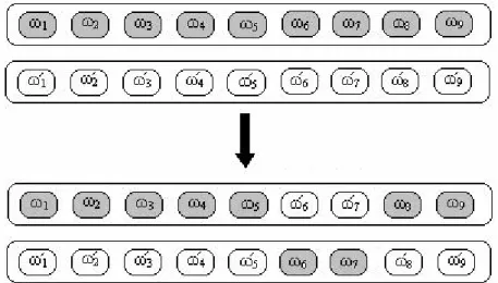
There are two kinds of reproduction in organisms. These are mitosis that is asexual reproduction and meiosis which is referred to sexual reproduction. Significant evolutionary changes can occur when genetic variability of a population is high, and this is usually the case for sexually reproducing organisms. Therefore, major mutation principles of sexual reproduction are adopted in GAs. Mutations that may occur during reproduction are the most important factors of evolution. There are two types of mutations: chromosome mutations and gene mutations. Crossover is the most important type of chromosome mutation used in GAs. In a crossover mutation two chromosomes swap their information at randomly selected corresponding points. This can be interpreted as an interchange of genes at respective points. On the other hand, gene mutations apply to a single gene of a chromosome, and it is the change of genetic information at this specific point. Figures 3 and 4 illustrate crossover and gene mutations respectively on the model’s linear information string. In fact there are more than one crossover types. However, we do not concentrate on details of crossover or other biological background of GAs. Here, the aim is to introduce the reader to basic principles.

(27)

Figure 3: A Crossover Example

Figure 4: A Gene Mutation Example

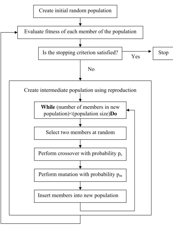
In the remaining part of this section how a GA operates will briefly be explained. It is noteworthy that we intensely make use of Chapter 2 of RJJ (1996) while explaining operation principles of GAs. Flow chart of a standard genetic algorithm is shown in Figure 5. The algorithm works as follows:

Step 1: Randomly create an initial population of chromosomes.

A GA starts by creating an initial population, which is filled with chromosomes that have randomly valued genes. Genes of an individual can be either binary or real-valued. In this thesis, they are real-valued and randomly chosen from a predefined interval. Population size, the number of chromosomes (individuals) contained in one

(28)

generation, is another parameter. Less than 50 chromosomes speed up convergence. However, this may cause a sub-optimal premature convergence. Therefore, in this thesis, the number of individuals is chosen as 50.

Create initial random population

Evaluate fitness of each member of the population

Figure 5: Flowchart of the Standard Genetic Algorithm (RJJ, 1996) Is the stopping criterion satisfied?

No

Stop

Create intermediate population using reproduction

While (number of members in new population)<(population size)Do

Select two members at random

Perform crossover with probability pc

Perform mutation with probability pm

Insert members into new population

(29)

Step 2: Compute the fitness of every member of the current population.

The fitness of every member of the current population is calculated through an evaluation (fitness) function. In this study, for each member of the population (a weight set for the neural network), a series of i for T =2000 is calculated through the network configuration, and c is obtained from equation (2). Then, the GA evaluates the outcome of the maximization problem given in equation (1), which is the fitness value of an individual. At the end of this step, GA has the fitness of each member in the current population. This step is the most time consuming part of the algorithm.

Step 3: If there is a member of the current population that satisfies the problem requirements then stop. Otherwise, continue with the next step.

The stopping requirement may be a sufficient solution to the problem or alternatively reaching a predefined number of generations.

Step 4: Create an intermediate population by extracting members from the current population using the reproduction or selection operator.

There are various selection operators. All selection operators that we utilize are designed to make their selections according to the fitness of members. Individuals with the highest fitness values have the highest probability of being selected.

Step 5: Generate a new population by applying the genetic operators, crossover and mutation, to this intermediate population.

The number of intermediate population members is smaller than the original population to create room for new members. Two random chromosomes are randomly selected from the intermediate population and are called parents. With a probability of crossover, pc, there occurs a crossover between the parents. After the

(30)

potential application of the crossover operator, each gene of the resulting chromosomes is subject to mutation with a probability of pm. After these genetic

manipulations, resulting chromosomes are inserted to the new population. If no genetic operation is applied, then the resulting chromosomes are the same with their parents. This procedure is repeated until the original population size is reached. An important point to mention is the use of elitism. Under elitism, the fittest member of the current population is directly transferred to the next generation, preventing the loss of a fittest member through genetic operations, once it is found.

(31)

CHAPTER 4 RESULTS

In this chapter, simulation results of different parameter configurations are presented. The following cases are simulated:

i. τ =δ =1, z =0 (benchmark case).

ii. τ ≠1, δ =0, z=0 (the case with different risk aversion values where no exact solution exists).

iii. Cases (i) and (ii) with positive capital adjustment costs,0<z.

Parameters of case (i) are the same with Duffy and McNelis’ (2001) benchmark parameter values providing a direct comparison opportunity. Case (ii) aims to compare our method’s performance with other methods’ presented in Taylor and Uhlig (1990). Case (iii) seeks the effects of capital adjustment costs under the same parameters with cases (i) and (ii).

For running the simulations we make use of Genesis 5.0, a free GA software package (Grefenstette, 1990). We compiled Genesis 5.0 on a Sun Microsystems Enterprise 4000 over UNIX operating system using a Telnet connection to the local area server. For each simulation we run the program once for 30000 generations with a population size of 50, a crossover probability of 0.6, and a mutation probability of 0.001. For all simulations the policy variable is approximated over T = 2000 periods.

(32)

With all these facts the simulation time is a little bit lengthy when compared to the other methods –especially the collocation methods. However, it must be considered that GA is a global search algorithm and searches a greater search space. Therefore, its results are more robust than the other methods. In fact, by picking well educated guesses of initial conditions like collocation methods do, for instance initial points very close to the steady state, GAs perform quite fast. The problem is alike fishing. While one method, GA, searches a fish flock in the whole sea, the other, for instance collocation, uses sonar and pinpoints the flock. The question is what if you do not have sonar?

4.1 Simulation Results of the Benchmark Case

This is the case where a closed-form solution of the problem in equation (1) exists. Therefore, the performance of our method is best observed in this case. The parameter values for this case are:

1 = =δ

τ , z =0, α = 0.33, ρ = 0.95, β∈

{

0.95,0.98

}

, σ ∈

{

0.01,0.05

}

.

The weight space is chosen as [-8, 8] when β = 0.95, and [-30, 30] when β = 0.98. For β = 0.95, the following pairs of initial values are fed into the neural network:

(

k0,θ0

)

= {(0.01, 0.83), (0.17, 1), (0.20, 0.9845), (0.06, 0.8560)} When β = 0.98, the following initial values are used:

(

k0,θ0

)

= {(0.1, 7.3), (0.5, 4.5), (1, 2.7), (1.5, 1), (2, 0.6), (2.5, 0.2), (3, 0.3), (3.5, 0.15)}.

β and σ values are the same with those of Duffy and McNelis’ (2001) giving an

occasion for a direct comparison of both models.

Since there is an exact solution under the benchmark case, the method’s approximation performance is evaluated most efficiently by a measure, which

(33)

compares the approximation of the optimal policy path with the exact one. Such a measure is proposed by Duffy and McNelis (2001) in the form of the following error statistic: 2 0 10

)

,

(

)

,

(

)

,

(

ˆ

1 log

)

(

∑

=

⎟

⎠

⎞

⎜

⎝

⎛

₋

=

T t k

f

k

f

k

f

N

f

e

θ

θ , (11)

where fˆ(k,θ) is the approximate consumption function and f (k,θ) is the actual

consumption function given in equation (9)4. Nk and Nθ stand for the number of grids that the policy function is evaluated over, and Nk = Nθ = 80. To generate the grid points, first, 80 equally spaced values of ε_tare picked up from the interval [-2σ, 2σ].

Then, the grid points for θ are recovered from ε_t grid points by using the long-run relation, lnθ = [1/(1-ρ)]ε , and then taking the exponent of lnθ. Next, the grid points

for k are generated by using the long-run relation between k and θ, k =

(

αβθ

)

1(1−α). There are 80 grid points for both k and θ. Thus, the error statistic is evaluated over

6400 different combinations of k and θ. e

( )

f is an easily interpretable measure of accuracy, which expresses the approximation error as a fraction of consumption. A result of -2 stands for an accuracy rate of 1 in 100, meaning that the approximation error costs 1 unit for every 100 units of consumption.

In addition, under the benchmark case, we are able to compute the correlation between the approximate and exact consumption series (correlation coefficient, corr-w-exact in Table 1). Other than those statistics, we present the volatility of the consumption series (con-vol), which is the standard deviation of the Hodrick-Prescott

4_{Although the policy function in our model is i, in order to keep correspondence with Duffy and}

McNelis’ (2001) results, in (11), we make use of the consumption path recovered from the policy function.

(34)

series, and the ratio of the variance of investment to the variance of the first difference of consumption (i-c ratio). The statistical results of benchmark simulations are given in Table 1 and the optimal network weights are given in Table 2.

Table 1: Statistics for the Benchmark Case

β = 0.95 β = 0.98

σ 0.01 0.05 0.01 0.05

Values for exact solution

con-vol 0.00684 0.03538 0.00685 0.03541

i-c ratio 2.88642 2.84652 3.16214 3.11843 Values for approximations

e( f ) -2.33 -0.62 -2.19 -1.25 Duffy&McNelis NN e( f )* _{-1.36 -0.26 -1.52 -0.24} Duffy&McNelis PA e( f ) -0.44 -0.38 -0.48 -0.39 corr-w-exact 0.99770 0.996611 0.99369 0.99784 con-vol 0.00679 0.03567 0.00674 0.03481 i-c ratio 2.23239 2.20580 12.55298 7.78099

*_{Duffy&McNelis NN stands for neural network approximation and PA stands for}

polynomial approximation

Table 2: Optimal Network Weights for the Benchmark Case

β = 0.95 β = 0.98 σ 0.01 0.05 0.01 0.05 ω1 0.618 1.275 -2.903 -1.026 ω2 -8.000 -6.123 -1.437 -2.199 ω3 2.213 -4.575 2.141 0.909 ω4 -6.217 7.844 -3.548 -2.610 ω5 2.307 -2.682 3.314 -3.490 ω6 3.918 -5.404 28.182 -4.721 ω7 7.906 4.903 4.018 -5.601 ω8 0.070 0.461 0.029 30.000 ω9 4.340 0.070 30.000 0.029

According to log10 average relative squared error, e( f ), in Table 1, our model’s

approximation accuracy is quite high and much better than the hybrid methodology of Duffy and McNelis (2001). However, accuracy decreases as σ increases.

(35)

is nearly perfect. Also, volatilities of both exact and approximate consumption paths (con-vol in Table 1) are nearly the same under all conditions. On the other hand i-c ratio is underestimated when β = 0.95, and overestimated when β = 0.98.

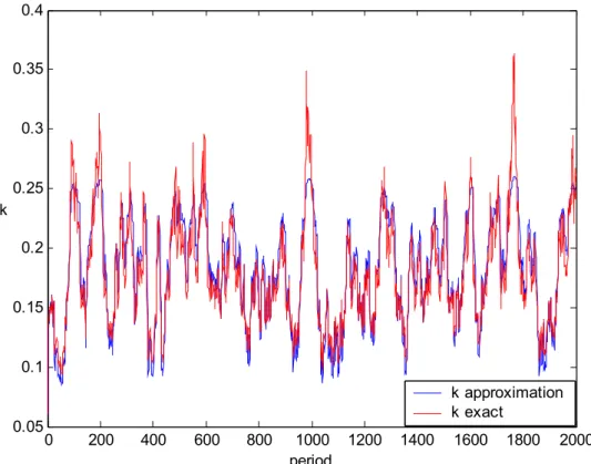
In addition to the statistical results, figures comparing the exact and approximate paths of capital and consumption series are quite explanatory in demonstrating the accuracy of our methodology. We do not present all such figures in this chapter since there are overwhelmingly many of them. Appendix A includes all figures. 0 200 400 600 800 1000 1200 1400 1600 1800 2000 0.15 0.16 0.17 0.18 0.19 0.2 period k k approximation k exact

Figure 6: Capital path for the benchmark case, σ = 0.01, β=0.95, k0=0.01

As seen by the figures, approximations to the capital and consumption paths are nearly perfect under different parameter combinations. However, with a greater sigma value approximation accuracy of the capital path, so the investment path (consider that i = kt+1 since there is full depreciation) decreases.

(36)

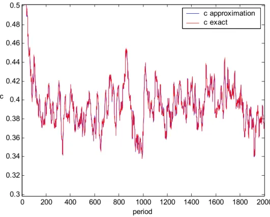
0 200 400 600 800 1000 1200 1400 1600 1800 2000 0.34 0.35 0.36 0.37 0.38 0.39 0.4 0.41 0.42 0.43 0.44 period c c approximate c exact

Figure 7: Consumption path for the benchmark case, σ = 0.01, β=0.95, k0=0.01

0 200 400 600 800 1000 1200 1400 1600 1800 2000 0.05 0.1 0.15 0.2 0.25 0.3 0.35 0.4 period k k approximation k exact

(37)

0 200 400 600 800 1000 1200 1400 1600 1800 2000 0.2 0.3 0.4 0.5 0.6 0.7 0.8 period c c approximation c exact

0 200 400 600 800 1000 1200 1400 1600 1800 2000 0.3 0.32 0.34 0.36 0.38 0.4 0.42 0.44 0.46 0.48 0.5 period c c approximation c exact

(38)

0 200 400 600 800 1000 1200 1400 1600 1800 2000 0.1 0.2 0.3 0.4 0.5 0.6 0.7 0.8 period c c approximation c exact

Figure 11: Consumption path for the benchmark case, σ = 0.05, β=0.98, k0=2

4.2 Simulation Results of Case (ii)

In this caseτ ≠1, δ =0, z=0, and there is no closed-form solution of the problem. The following parameter values are used in simulations:

{

0.5,1.5, 3

}

=

τ , α = 0.33, ρ = 0.95,β =0.95,σ =0.02.

These values are the same with the ones used in Taylor and Uhlig’s (1990) article. The weight space is [-30, 30]. The following initial values of k and θ are imposed to the neural network:

(

k0,θ0

)

= {(10, 0.82), (11, 1), (12, 1.22), (13, 0.82), (14, 1), (15, 1.22), (16, 0.82), (17, 1), (18, 1.22), (19, 0.82), (20, 1), (21, 1.22)}.

Since there is no exact solution in this case, we are not able to comment on the accuracy of our method by comparing it with the exact solution. Instead, we apply

(39)

four statistical tests. These are den Haan-Marcet statistic, the TR2 statistics, the R2 statistic, and Euler equation errors. First three of these statistics are defined by Taylor and Uhlig (1990) and the last one is proposed by Judd (1992). Also, con-vol and i-c ratio statistics are presented for this case too.

The den Haan-Marcet (1994) statistic, hereafter DM-stat, provides a test for the martingale-difference property of the Euler equation residual. It is computed in the following way: DM-stat ₌aˆ_′(x_′x)(x_′x_η2)−1(x_′x)aˆ_, 2 1 ) ( ˆ xx xη a= ′ − ′ τ α τ _αθ _δ β η − − − − − ₊ ₋ ₋ = 1 ₁ 1 1 ) ( _t _t _t t t c k c , (12)

where aˆ is the usual OLS estimator in a regression of the Euler equation residual η_t on x. Here, x is a matrix of instrumental variables consisting of 5 lags of consumption and θ, and a constant. Under the null hypothesis, which is an accurate approximation to the optimal path, the DM-stat has a Chi-square distribution with degrees of freedom equal to number of instrumental variables. In calculating the DM-stat, we use the same instruments that Taylor and Uhlig (1990) uses, so a direct comparison with other models presented in their paper is possible. Under the null hypothesis, the DM-stat has an asymptotic χ2(11) distribution with critical values [3.81, 21.92] at the 5% level, and [3.05, 24.72] at the 1% level of significance.

The TR2 statistic is obtained from a regression of the productivity shockε_ton 5 lags of consumption, capital and θ. TR2 is used to test for the martingale-difference property,E_t₋₁ε_t =0. The TR2 statistic is calculated in the following way:

[

]

, ) ˆ ˆ ( ) ( ) ˆ ˆ )( ( 2 2 2 2

∑

− − − − = t t t t t t t t T TR ε ε ε ε ε ε ε ε (13)

(40)

b x_t t = ˆ ε , t t t tx x x b_ˆ=₍ ′ ₎−1 ′ε _{, (13)} where T is the number of observations, 2000, and xt is the vector of lagged variables.

Under the null hypothesis of E_t₋₁ε_t =0, TR2 statistic has an asymptotic χ2(15) distribution. The critical bounds at the 5% significance level are [6.26, 27.49].

R2 statistic from the regression of the first difference of consumption on both lagged consumption and capital is a test for the random walk hypothesis of consumption. An R2 close to zero is accepted as an evidence for the random walk hypothesis.

Euler equation error, which is similar to e( f ), is another measure of accuracy defined by Judd (1992). Hereafter, we call this measure as Judd Criterion, JC. JC is a scale free measure of the average intertemporal error an agent would make using the approximate solution. A value of -2 means that the approximation error costs 1 unit for every 100 units consumed. It is computed in the following way:

(

)

[

]

⎭

⎬

⎫

⎩

⎨

⎧

₊

₋

−

=

−+ +₋ +− τ α τ

_αθ

_δ

β

t t t t t

c

k

c

E

JC

log

1

1 1 1 1 10 (14)

Graphical demonstration of JC results is more illustrative. In the figures, values of capital are ranging within the interval [(1−∆_k)k*;(1+∆_k)k*], where k* is the deterministic steady state and ∆k =0.2, and values of the technology shock guarantees that 95% of the distribution of ln(θt) is covered. A 20 nodes

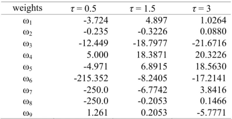
Gauss-Hermite quadrature is used to evaluate the integral involved by the expectation. Optimal network weights are in Table 3, and the statistical results are presented in Table 4.

(41)

Table 3: Optimal Network Weights for Case (ii) weights τ = 0.5 τ = 1.5 τ = 3 ω1 -3.724 4.897 1.0264 ω2 -0.235 -0.3226 0.0880 ω3 -12.449 -18.7977 -21.6716 ω4 5.000 18.3871 20.3226 ω5 -4.971 6.8915 18.5630 ω6 -215.352 -8.2405 -17.2141 ω7 -250.0 -6.7742 3.8416 ω8 -250.0 -0.2053 0.1466 ω9 1.261 0.2053 -5.7771

Table 4: Statistics for Case (ii)

τ = 0.5 τ = 1.5 τ = 3 DM-stat 49.3404 22.6080 35.9537 TR2 _16.0029 _11.5066 _12.6382 R2 0.0210 0.0034 0.0047 JC -2.1854 -2.4673 -2.7208 i-c ratio 1.0514 19.3964 8.7246 con-vol 0.0414 0.0292 0.0317

According to the results in Table 4, among all simulations only the one with τ = 1.5 satisfies the DM-stat in the 1% significance level. In contrast, at all τ values TR2 statistic is within the critical boundaries, and R2 is nearly zero, i.e. supports random walk hypothesis of consumption. Moreover, for all τ values JC is under -2 pointing a quite reasonable rate of cost. Figures of JC prove how successful the approximation accuracy is. Furthermore, consumption volatilities and i-c ratios are consistent with the fact that the volatility of consumption has to decrease so i-c ratio increase with an increasing risk aversion coefficient. However, there is an inconsistency of i-c ratios between τ =1.5and τ =3cases.

(42)

-0.2 0 0.2 12 14 16 18 20-7 -6 -5 -4 -3 -2 -1 logtheta k JC

Figure 12: JC - log10 |Euler residual| for case (ii), τ = 0.5

-0.2 0 0.2 12 14 16 18 20-6 -5 -4 -3 -2 -1 logtheta k JC

(43)

-0.2 0 0.2 12 14 16 18 20-7 -6 -5 -4 -3 -2 logtheta k JC

Figure 14: JC - log10 |Euler residual| for case (ii), τ = 3

Table 5 compares our method with the methods in Taylor and Uhlig (1990) and Duffy and McNelis (2001). In Table 5, our model is represented as GA-NN (Genetic Algorithm-Neural Network). The methods that we compare with our method are Duffy and McNelis’ (2001) parameterized expectation approach using GA-gradient descent hybrid methodology for both neural network and polynomial approximations, log-linear quadratic and linear quadratic methods of Christiano (1990) and McGratten (1990), the backward solutions of Ingram (1990) and Sims (1990), the parameterized expectations approach of den Haan and Marcet (1990) and the quadrature method of Tauchen (1990). According to Table 5, our GA-NN method performs quite well. In fact, our model is the only one that exposes random walk behavior of consumption under all configurations.

(44)

Table 5: Comparison with Other Methods A: τ = 0.5

DM-stat TR2 _R2_i-c_ratio

GA-NN 49.34 16.003 0.02 1.0514 Duffy-McNelis NN 35.46 13.69 0.02 9.75 Duffy-McNelis PA 34.38 12.63 0.07 5.77 Christiano-Loq LQ 17 10 0.43 29 Ingram 10 17 0.44 30 den Haan-Marcet 18 15 0.42 30 McGratten 96 19 0.34 24 Sims 12 24 0.44 31 Tauchen 704 11 0.50 3 B: τ = 1.5

GA-NN 22.61 11.507 0.0034 19.3964 Duffy-McNelis NN 7.98 11.09 0.03 9.92 Duffy-McNelis PA 36.12 14.09 0.07 3.24 Christiano-Loq LQ 10 10 0.05 11 Ingram 11 165 0.06 12 den Haan-Marcet 18 14 0.06 13 McGratten 22 19 0.04 9 Sims 12 24 0.07 13 Tauchen 558 9 0.38 2 C: τ = 3

GA-NN 35.95 12.638 0.0047 8.7245 Duffy-McNelis NN 2.34 11.46 0.05 13.28 Duffy-McNelis PA 25.96 15.42 0.04 1.94 Christiano-Loq LQ 18 19 0.02 8 Ingram 12 394 0.03 20 den Haan-Marcet 12 13 0.03 10 McGratten 17 19 0.02 7 Sims 12 22 0.04 11 Tauchen 502 14 0.33 2

4.3 Simulations for Case (iii): Capital Adjustment Costs

In this case, we simulate the benchmark case and case (ii) by introducing positive capital adjustment costs to the model, i.e. 0< z. This simulation helps to

(45)

understand how successful the GA-NN method is in mimicking certain economic facts. For instance, before running this case, a decrease in the volatility of physical capital investment was expected with the introduction of positive capital adjustment costs. Later, this behavior is observed in model’s solutions.

For comparison with the benchmark case the following parameter configurations are simulated:

} 1 . 0 , 05 . 0 , 025 . 0 { , 95 . 0 , 01 . 0 , 1 = = ∈ = =δ σ β z τ

All other parameters, including the initial conditions, are the same with the corresponding benchmark case’s parameters. The parameter configurations for comparison with case (ii) are:

} 1 . 0 , 05 . 0 , 025 . 0 { , 95 . 0 , 02 . 0 , 0 , 5 . 1 = = = ∈ = δ σ β z τ

with all other parameters being the same with analogous parameters of case (ii).

4.3.1 Benchmark Case with Capital Adjustment Costs

In the benchmark case, we interpret the effects of adjustment costs by three statistics. These are consumption volatility (con-vol in Table 6), variance of investment (ivar in Table 7) and i-c ratio (Table 6). Variance of investment is simply equal to the variance of the first difference of capital series. Also, we utilize the Judd Criterion (JC in Table 6) as an accuracy check for solutions. It is calculated in the following way:

(

)

[

(

)(

)

]

⎭

⎬

⎫

⎩

⎨

⎧

₊

₋

₊

−

+

=

−+ + +−₋ τ α τ

_αθ

_δ

β

t t t t t t t

c

zi

k

c

E

zi

JC

log

1

1 1 1 1 10 (15)

Consumption volatility (con-vol in Table 6) is expected to increase with the introduction of capital adjustment costs. That is because positive production shocks are expected to be balanced by changes in consumption rather than investment since

(46)

physical capital investment is costly. Therefore, the response of investment to production shocks is expected to decrease resulting in a smoother investment path. So, a decrease in the variance of investment path is expected. Moreover, i-c ratio, the ratio of the variance of investment to the variance of the first difference of consumption, is expected to decrease as a result of decreasing investment variance and increasing consumption volatility.

Table 6: Statistical Effects of Capital Adjustment Costs

z = 0 z = 0.025 z = 0.05 z = 0.1 con-vol 0.00679 0.00712 0.00710 0.00709 i-c ratio 2.23239 0.51005 0.55775 0.42186

JC NA -2.2715 -2.2718 -2.2724

Table 7: Comparison of Investment Variances ivar

z = 0 z = 0.025 z = 0.05 z = 0.1

k0 = 0.01 1.1561e-004 5.1849e-005 1.2582e-005 4.7350e-005

k0 = 0.06 1.0742e-004 3.1990e-005 3.3170e-005 2.8065e-005

k0 = 0.17 8.0052e-005 1.1709e-005 5.2058e-005 9.8383e-006

k0 = 0.20 9.2659e-005 1.7337e-005 1.8507e-005 1.4709e-005

In Table 6, consumption volatility slightly increases with the introduction of adjustment costs. In addition, i-c ratio decreases remarkably. Moreover, JC points reasonable approximation accuracy. Also, graphical demonstrations of JC bring a more explanatory viewpoint to the approximation accuracy. Furthermore, investment variances in Table 7 satisfy the expectation that the volatility of investment path decreases with positive adjustment costs. On the other hand, there is an inconsistency between different levels of adjustment costs. For instance, while higher consumption volatility was expected for higher adjustment cost, we observed slightly lower volatility. Again, i-c ratio of z = 0.05 is a little higher than z = 0.025.

(47)

0 200 400 600 800 1000 1200 1400 1600 1800 2000 0.16 0.17 0.18 0.19 0.2 0.21 0.22 period k z = 0 z = 0.025

Figure 15: Benchmark capital path with and without adjustment costs, k0=0.17

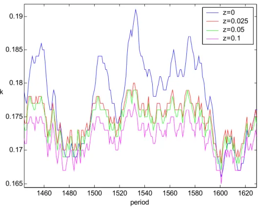
1460 1480 1500 1520 1540 1560 1580 1600 1620 0.165 0.17 0.175 0.18 0.185 0.19 period k z=0 z=0.025 z=0.05 z=0.1

(48)

Last but not the least, figures of capital path illustrates the effects of adjustment costs. Figure 15 is an evidence for the decrease of volatility in the capital path due to positive adjustment costs. In Figure 16, all paths have the same parameter values initial conditions and θ series. The figure shows that the higher the adjustment cost is the lower the investment path volatility. Figure 17 demonstrates the Judd Criterion for the benchmark case. All other figures for the benchmark case with adjustment costs are available in Appendix C.

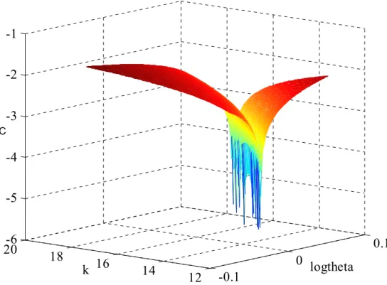
-0.1 0 0.1 12 14 16 18 20-6 -5 -4 -3 -2 -1 logtheta k JC

Figure 17: JC - log10|Euler residual| for the benchmark case with z = 0.025

4.3.2 Case (ii) with Capital Adjustment Costs

Expectations for this case is no different than the benchmark case with capital adjustment costs, i.e. a higher consumption volatility is expected while relative volatility of consumption and investment (i-c ratio) is expected to decrease. For this case we compute TR2, R2, consumption volatility (con-vol), i-c ratio and Judd

(49)

criterion (JC) statistics. The reason for computing TR2 and R2, and the calculation way of these statistics are exactly the same as in case (ii). JC is calculated as in equation (15). con-vol and i-c ratio are computed for different adjustment cost coefficients and compared with the corresponding values of case (ii). Also, figures of JC are plotted. All statistics are presented in Table 8.

Table 8: Statistics for Case (ii) with Capital Adjustment Costs

z = 0 z = 0.025 z = 0.05 z = 0.1 TR2_11.5066 _16.3639 _13.9377 _19.8971 R2_0.0034 _0.0065 _0.0099 _0.0079 con-vol 0.0292 0.0344 0.0348 0.0361 i-c ratio 19.3964 6.8881 9.9624 5.7457 JC -2.46726 -2.50933 -2.41209 -2.58274 -0.2 0 0.2 12 14 16 18 20-7 -6 -5 -4 -3 -2 -1 logtheta k JC

Figure 18: JC - log10|Euler residual| for case (ii) with z = 0.025

For all levels of adjustment cost, TR2 statistic is within the 5% significance level boundaries, [6.26, 27.49], satisfying the martingale difference property,

(50)

0

1 =

− t t

E ε . R2 values in Table 8 support the random walk hypothesis of consumption. Consumption volatility and i-c ratio are in line with the expectations, but there is, again, an inconsistency of i-c ratios among different adjustment costs. JC values represent a quite reasonable accuracy of approximation for all levels of adjustment costs. Figure 18 illustrates the JC- log10|Euler residual| for z = 0.025. Figures for other levels of adjustment costs are presented in Appendix D.

(51)

CHAPTER 5 CONCLUSION

This thesis proposed a powerful solution methodology for the one-sector non-linear stochastic optimal growth problem. The proposed method utilizes a neural network trained by a genetic algorithm. Therefore, we named it as GA-NN method. The vast global search skills of genetic algorithms combined with the great modeling ability of neural networks makes the GA-NN method quite potent in solving the problem.

The model is simulated under three different sets of parameters, i.e. three cases. Two of these cases provided a comparison with other methods, whereas the third one enlarged the space of study to a more realistic environment by adding positive capital adjustment costs to the model. The first one was the benchmark case, in which there is a closed-form solution. In this case, GA-NN method’s approximation accuracy dominated the accuracy of Duffy and McNelis’ (2001) hybrid methodology. Also, consumption volatilities are almost the same with the exact solution’s, and correlation with the exact solution is so high that in figures comparing the exact and approximate consumption paths it is hard to distinguish the two paths.

The second case was exactly the same as in Taylor and Uhlig (1990). GA-NN method performed quite well and satisfied the criteria of all statistics, except the den Haan-Marcet statistic. Furthermore, GA-NN method turned out to be the only one

(52)

that supports the random walk hypothesis of consumption. Moreover, the method produced quite reasonable levels of approximation accuracy with respect to the Judd criterion.

In the third case, we introduced capital adjustment costs to the model and simulated the benchmark case and the second case with these costs. The outcomes of these simulations were in line with the expectations. With the introduction of costs, consumption volatility increased and investment volatility decreased for both cases. Investment was observed to respond less to positive productivity shocks when adjustment costs were present. Judd criterion values point quite good approximation accuracy for both cases. By looking at these results, it can be said that GA-NN solution methodology is successful in more realistic environments too.

Unlike the existing solution methods, GA-NN method does not need to solve for the Euler equation providing a great practicality to the user. Instead of dealing with the Euler equation, GA-NN method directly deals with parameterizing the policy function with neural networks. It is a fact that the computation time for GA-NN method is longer than other methods. However, it must be considered that other methods require solving for the Euler equation by hand, and when the number of parameters entering the model increases, the required time for this process increases much more. Moreover, the existence of some derivatives is uncertain when the dimension of the search space folds, even putting doubt on the solution ability of the models using the Euler equation. Since GA-NN method is free of all these problems, it is much more robust than the so called fast methods. Also, the computer systems that were used in this thesis study were relatively slow with respect to the existing computer technologies. If speed were everything, we would have utilized the super computer technologies of today.

(53)

Future extensions to this thesis study are possible. Irreversibility of physical capital can be put as a constraint to the model. Actually, irreversibility was proposed by Sargent (1980) as another form of capital adjustment costs. Addition of debt to the model is another extension. Adding other parameters can enhance the reality of the model. Moreover, it is possible to use parallel genetic algorithms to speed up the simulation process of the method.

(54)

SELECT BIBLIOGRAPHY

Alemdar, N.M., S. Sirakaya, S.J. Turnovsky. 2006. “Feedback Approximation of the Stochastic Growth Model by Genetic Neural Networks,” Forthcoming in

Computational Economics.

Baxter, M., M.J. Crucini, and K.G. Rouwenhorst. 1990. “Solving the Stochastic Growth Model: A Discrete State Space, Euler Equation Approach,” Journal

of Business and Economic Statistics 8: (19-21)

Brock, W.A., and L. Mirman. 1972. “Optimal Economic Growth and Uncertainty: the Discounted Case,” Journal of Economic Theory 4: 479-513.

Caballero, R. 1999. ”Aggregate Investment.” In J. Taylor and M. Woodford, eds.,

Handbook of Macroeconomics. Amsterdam: North Holland

Christiano, L.J. 1990. “Solving the Stochastic Growth Model by Linear Quadratic Approximation and by Value Function Iteration,” Journal of Business and

Economic Statistics 8: 99-113.

Cooper, R.W., and J.C. Haltiwanger. 2000. “On the Nature of Capital Adjustment Costs.” NBER Working Paper No 7925.

Den Haan, W., and A. Marcet. 1990. “Solving the Stochastic Growth Model by Parameterizing Expectations,” Journal of Business and Economic Statistics 8: 31-34.

Duffy, J., and P.D. McNelis. 2001. “Approximating and Simulating the Stochastic Growth Model: Parameterized Expectations, Neural Networks, and the Genetic Algorithm,” Journal of Economic Dynamics and Control 25: 1273-1303.

Grefenstette, J.J. 1990. “A User’s Guide to GENESIS Version 5.0.” Manuscript. Holland, J.H. 1975. Adaptation in Natural Artificial Systems. Ann Arbor, MI: The

University of Michigan Press.

Hornik, K., M. Stinchcombe, and H. White. 1989. “Multilayer Feedforward Networks are Universal Approximators,” Neural Networks 2: 359-366.

(55)

Ingram, B.F. 1990. “Solving the Stochastic Growth Model by Backsolving with an Expanded Shock Space,” Journal of Business and Economic Statistics 8: (37-38)

Judd, K.L. 1992. “Projection Methods for Aggreagate Growth Models,” Journal of

Economic Theory 58: 410-452.

Judd, K.L. 1998. Numerical Methods in Economics. Cambridge MA: MIT Press. McGrattan, E.R. 1990. “Solving the Stochastic Growth Model by Linear-Quadratic

Approximation,” Journal of Business and Economic Statistics 8: 41-44

Mendoza, E.G. 1991. “Real Business Cycles in a Small Open Economy,” The

American Economic Review 81(4): 797-818.

Miranda, J.M., and P.L. Fackler. 2002. Applied Computational Economics and

Finance. Cambridge MA: MIT Press.

Rooij, A.J.F., L.C. Jain, and R.P. Johnson. 1996. Neural Network Training Using

Genetic Algorithms. Singapore: World Scientific.

Sargent, Thomas J. 1980. “Tobin’s q and the Rate of Investment in General Equilibrium.” Carnegie-Rochester Conference Series on Public Policy 12: 107-54.

Sargent, Thomas J. 1987. Dynamic Macroeconomic Theory. Cambridge MA: Harvard University Press.

Sims, C.A. 1989. “Solving Nonlinear Stochastic Optimization and Equilibrium Problems ‘Backwards’.” Discussion paper No. 15, Institute for Empirical Macroeconomics, Federal Reserve Bank of Minneapolis.

Sims, C.A. 1990. “Solving the Stochastic Growth Model by Backsolving with a Particular Nonlinear Form for the Decision Rule.” Journal of Business and

Taylor, J.B., and H. Uhlig. 1990. “Solving Nonlinear Stochastic Growth Models: A Comparison of Alternative Solution Methods,” Journal of Business and

Tauchen, G. (1990). “Solving the Stochastic Growth Model by Using Quadrature Methods and Value Function Iterations,” Journal of Business and Economic

Statistics 8: 49-51.

Zaruda, Jacek M. 1992. Introduction to Artificial Neural Systems. New York: West Publishing Company.

(56)

APPENDIX A

FIGURES FOR THE BENCHMARK CASE

0 200 400 600 800 1000 1200 1400 1600 1800 2000 0.15 0.16 0.17 0.18 0.19 0.2 period k k approximate k exact

(57)

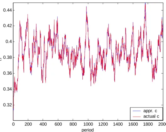
0 200 400 600 800 1000 1200 1400 1600 1800 2000 0.32 0.34 0.36 0.38 0.4 0.42 0.44 period c appr. c actual c

0 200 400 600 800 1000 1200 1400 1600 1800 2000 0.15 0.16 0.17 0.18 0.19 0.2 0.21 0.22 period k k approximate k exact

(58)

0 200 400 600 800 1000 1200 1400 1600 1800 2000 0.34 0.36 0.38 0.4 0.42 0.44 0.46 0.48 period c c approximate c exact

0 200 400 600 800 1000 1200 1400 1600 1800 2000 0.15 0.16 0.17 0.18 0.19 0.2 0.21 period k k approximate k exact

(59)

0 200 400 600 800 1000 1200 1400 1600 1800 2000 0.32 0.34 0.36 0.38 0.4 0.42 0.44 0.46 period c c approximate c exact

0 200 400 600 800 1000 1200 1400 1600 1800 2000 0.1 0.15 0.2 0.25 0.3 period k k approximate k exact

(60)

0 200 400 600 800 1000 1200 1400 1600 1800 2000 0.2 0.3 0.4 0.5 0.6 0.7 period c approximate c exact

0 200 400 600 800 1000 1200 1400 1600 1800 2000 0.05 0.1 0.15 0.2 0.25 0.3 0.35 0.4 0.45 period k k approximate k exact

(61)

0 200 400 600 800 1000 1200 1400 1600 1800 2000 0.2 0.3 0.4 0.5 0.6 0.7 0.8 0.9 1 period c c approximate c exact

0 200 400 600 800 1000 1200 1400 1600 1800 2000 0.05 0.1 0.15 0.2 0.25 0.3 0.35 0.4 period k k approximate k exact

Approximating the stochastic growth model with neural networks trained by genetic algorithms

ABSTRACT

ÖZET

ACKNOWLEDGMENTS

TABLE OF CONTENTS

LIST OF TABLES

LIST OF FIGURES

CHAPTER I

INTRODUCTION

CHAPTER 2

THE MODEL

⎥

⎦

⎤

⎢

⎣

⎡

−

∑

1

c

E

τ

β

k

i

k

k

i

z

i

c

)

1

(

2

δ

θ

−

+

=

=

+

+

θ

ρ

θ

ε

θ

(

)

[

β

αθ

δ

]

(

)

[

(

(

)(

)

)

]

zi

E

c

k

zi

c

1

+

=

β

αθ

+

1

−

δ