An Analytical Solution to the Stance Dynamics of Passive Spring-Loaded Inverted Pendulum with Damping
M. M. ANKARALI
Dept. of Electrical and Electronics Eng., Middle East Tech. University, Ankara 06531, Turkey
E-mail: [email protected] O. ARSLAN∗and U. SARANLI† ∗Dept. of Electrical and Electronics Eng.,
†Dept of Computer Engineering, Bilkent University, Bilkent Ankara 06800, Turkey E-mail:∗[email protected],†[email protected]
The Spring-Loaded Inverted Pendulum (SLIP) model has been established both as a very accurate descriptive tool as well as a good basis for the design and control of running robots. In particular, approximate analytic solutions to the otherwise nonintegrable dynamics of this model provide principled ways in which gait controllers can be built, yielding invaluable insight into their sta-bility properties. However, most existing work on the SLIP model completely disregards the effects of damping, which often cannot be neglected for physi-cal robot platforms. In this paper, we introduce a new approximate analytiphysi-cal solution to the dynamics of this system that also takes into account viscous damping in the leg. We compare both the predictive performance of our ap-proximation as well as the tracking performance of an associated deadbeat gait controller to similar existing methods in the literature and show that it significantly outperforms them in the presence of damping in the leg. Keywords: SLIP, damping, legged locomotion, running robots, deadbeat con-trol, analytical return maps
1. Introduction
Legged robot morphologies offer clear advantages on rough, outdoor terrain both in terms of the robustness and the diversity of their feasible locomotory behaviors. However, in light of complexities and inefficiency associated with slow, purely kinematic morphologies, it is fairly clear that legged systems can simultaneously achieve speed, agility and efficiency only by adopting dynamic modes of operation such as running and leaping. In this context,
the Spring-Loaded Inverted Pendulum (SLIP) model is widely accepted in the literature as a very successful descriptive dynamical model for such behaviors.1–3 Not surprisingly, the same model has also been used as the basis of numerous robots capable of dynamic locomotion.4–8
Nevertheless, despite the apparent simplicity of this model, its dynamics during stance are nonintegrable, motivating a number of analytical approxi-mations to support the analysis of its behaviors and the design of associated controllers.3,8–11In this paper, we introduce a new analytical approximation method which takes into account damping in the leg, a dominant element for any physical legged robot often completely ignored by existing methods. We show that when the effects of damping are not neglected, our method sig-nificantly outperforms existing approximations in the literature3,10,12both in its prediction of the stance map as well as its performance as a feed forward model within locomotion controllers.
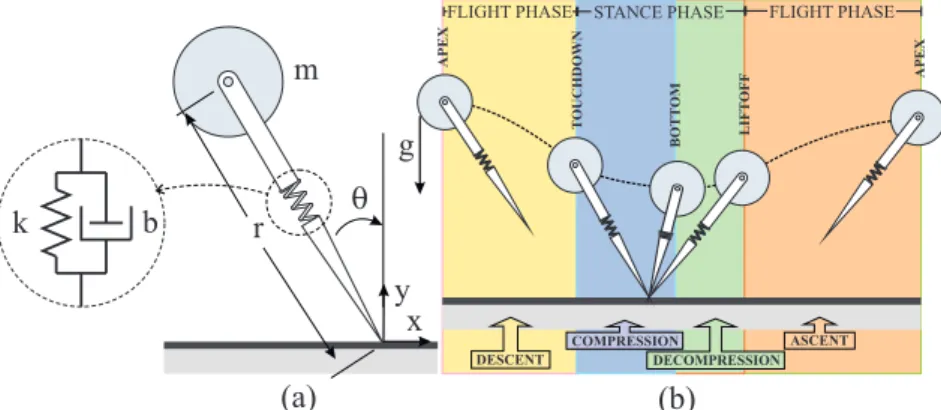
Fig. 1. The SLIP Model. (a) Coordinates and model parameters. (b) Locomotion phases (shaded regions) and transition events (boundaries).
2. The SLIP Model and Dynamics
Fig. 1 illustrates SLIP model we use, consisting of a point mass attached to a compliant, massless leg with viscous damping. Throughout locomotion, the model alternates as usual between stance and flight phases, which are further divided into compression, decompression and ascent, descent sub-phases respectively. Four important events define transitions between these subphases: touchdown, as the leg comes into contact with the ground, bot-tom, as the leg reaches its maximum compression, liftoff, as the toe takes off from the ground and finally apex, as the body reaches its maximum height during flight. Table 1 details the notation used throughout the paper.
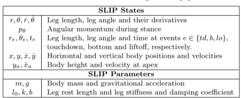
Table 1. Notation used throughout the paper SLIP States
r, θ,˙r, ˙θ Leg length, leg angle and their derivatives pθ Angular momentum during stance
re, θe, te Leg length, leg angle and time at events e ∈ {td, b, lo}, touchdown, bottom and liftoff, respectively.
x, y,˙x, ˙y Horizontal and vertical body positions and velocities ya,˙xa Body height and velocity at apex
SLIP Parameters
m, g Body mass and gravitational acceleration
l0, k, b Leg rest length and leg stiffness and damping coefficient
During flight, the body follows a ballistic trajectory, whereas during stance, the toe remains stationary on the ground with no torque applied to the leg. The stance dynamics of this model in polar leg coordinates are
m¨r = mr ˙θ2+ k(l0− r) − mg cos(θ) − b ˙r , (1) 0 = d
dt(mr
2˙θ) + mgr sin θ . (2)
Subsequent sections present our analytical approximations to these dynam-ics as well as an associated deadbeat controller for SLIP running.
3. An Approximate Stance Map for SLIP with Damping
In deriving our analytical approximation to the stance dynamics of the SLIP model, we make the commonly used assumption that the leg remains close to the vertical throughout the entire stance phase. Consequently, the effects of gravity can be linearized around θ = 0. The resulting conservation of the angular momentum pθ:= mr2˙θ reduces the radial dynamics to
¨
r + b ˙r/m + kr/m − p2
θ/(m2r3) = −g + kl0/m . (3) Unfortunately, even these reduced dynamics do not admit an analytical solution. However, inspired by the method proposed by Geyer,10we further assume that the relative spring compression, defined as l0−r
l0 ≪ 1, remains
sufficiently small that the term 1/r3can be approximated by a Taylor series expansion around l0, resulting in
1/r3¯¯
r=l0 ≈ 1/l
3
0− 3/l40(r − l0) + O((r − l0)2) . (4) Under this approximation, (3) is reduced to
¨
r + (b/m) ˙r + (ω02+ 3ω2)r = −g + l0ω20+ 4l0ω2, (5) where we define ω := (pθ)/(ml02) and ω0:=pk/m. In order to solve (5) in a more compact form, we define ˆω0:=
√
ζ := b/(2mˆω0) and ωd:= ˆω0p1 − ζ2. Assuming ζ < 1, we then have r = e−ζ ˆω0t
(A cos(ωdt) + B sin(ωdt)) + F/ˆω02, (6) with A and B determined by touchdown states, rtd and ˙rtd, as
A = rtd− F/ˆω20, B = ( ˙rtd+ ζ ˆω0A)/ωd. Simple differentiation yields the radial velocity as
˙r = −M e−ζ ˆω0t
(ζ ˆω0cos(ωdt + φ) + ωdsin(ωdt + φ)) , (7) where M := √A2+ B2 and φ := arctan(−B/A). Defining a new phase value, φ2 := arctan(−p1 − ζ2/ζ), the simplest form of the radial motion can be obtained as
r(t) = M e−ζ ˆω0t
cos(ωdt + φ) + F/ˆω02, (8) ˙r(t) = −M ˆω0e−ζ ˆω0tcos(ωdt + φ + φ2) . (9) Now that an analytical approximation to the radial trajectory is avail-able, the angular trajectory can be determined using the constant angular momentum ˙θ = pθ/(mr2). To this end, we linearize the term 1/r2 around the rest length of the leg spring as
1/r2¯ ¯r=l
0 = 1/l
2
0+ 2/l30(r − l0) + O((r − l0)2) , (10) and obtain an analytical solution for the rate of change of the leg angle as ˙θ(t) = 3ω − 2ωF/(l0ωˆ20) − 2ωMe−ζ ˆω0tcos(ωdt + φ)/l0, (11) whose integral can then be used to determine the angular trajectory
θ(t) = θtd+ X t + Y (e−ζ ˆω0t cos(ωdt + φ + φ3) − cos(φ + φ3)) , (12) where X := 3ω − 2ωFl0ωˆ02, Y :=
2ωM
l0ωˆ0 and φ3 := arctan(p1 − ζ
2/ζ). These approximations yield a sufficiently simple analytic solution to the stance dynamics of the SLIP model with damping, leaving only the determination of times at which the critical bottom and liftoff events occur during stance. 4. Times for Critical Events: Bottom and Liftoff
The bottom event is defined as the time at which the leg reaches its maxi-mum compression with ˙r(tb) = 0. Using (9), this yields the solution
tb = (π/2 − φ − φ2)/ωd. (13)
In contrast, the liftoff event occurs when the toe loses contact with the ground. Normally, when no damping is present in the leg with ζ = 0, (6)
becomes r = M cos(ˆω0 + φ) + F/ˆω02, and an analytical solution for the liftoff time can easily be obtained. However, when damping is present in the system, the calculation of the liftoff time is considerably more difficult. This is because, regardless of the leg length, the SLIP toe leaves the ground when the ground reaction force induced by the leg crosses zero and starts to become negative. As a result, the liftoff time is computed as
k(l0− r(tc1lo)) − b ˙r(tc1lo) = 0 . (14) On the other hand, there are also cases where liftoff may be caused by explicit constraints imposed by the morphology of particular robots such as the BowLeg hopper.8 In this paper, we also allow explicit choice of the liftoff length, rloby a high-level gait controller. In this case, the liftoff time is determined by the solution to the equation
r(tc2lo) = rlo. (15)
The actual liftoff time can then be found as tlo = min(tc1lo, tc2lo). Un-fortunately, exact analytical solution of these equations is not possible and numerical methods, which are feasible due to the simple, one dimensional nature of these equations, need to be adopted.
Nevertheless, in order to preserve the fully analytic nature of the SLIP return map, we use a sufficiently accurate analytical approxima-tion to compute both liftoff times. Since the exponential term multiply-ing the radial solution of (8) is the main source of the problem, we ap-proximate it with its value at a specific instant during decompression as e−ζ ˆω0t
≈ e−ζ ˆω0γtb, where γ ≥ 1 is a tunable parameter. A reasonable choice
is γ = 1+(rlo−rb)/(l0−rb), which incorporates the relative ratios of touch-down and liftoff lengths to estimate the liftoff time. Under this assumption, we have tc1lo ≈ (2π − arccos(k(l0− F/ˆω20)/(M M e−ζ ˆω 0γtb)) − φ − φ 4)/ωd, (16) tc2lo ≈ (2π − arccos((l0− F/ˆω20)/(M e−ζ ˆω 0γtb)) − φ)/ω d, (17)
where M := p(bˆω0)2+ k2− 2kbˆω0cos(φ2) & φ4 := arctan(bˆωb0ωˆ0cos(φsin(φ2)−k2) ).
Finally, we perform a small correction on the liftoff angular velocity to ac-count for the energy difference erroneously indiced by our approximations. While it is also possible to use gravity corrections on the angular momen-tum,11the effect of this linearization is minimal compared to damping losses and this simple correction proved to be more than adequate.
5. Simulation Results
5.1. Predictive Performance
In order to assess the performance of our method, we simulated a single stride of the SLIP model using a range of different initial conditions and damping coefficients, and compared its predictions to Geyer’s10analytic ap-proximations. All simulations were done with m = 1 and rtd= rl0= l0= 1, together with initial conditions and remaining parameters accordingly scaled to be representative of natural runners, yielding 94248 simulations covering ˙x ∈ [1, 5](m/s), y ∈ [1.15, 1.75](m), k ∈ [250, 2000](N/m), θtdrel ∈
[−0.150.25](rad.) and ζ0 := b/(2 √
mk) ∈ [0, 0.5], where θtdrel denotes the
deviation of the touchdown angle from its value that would result in a neu-tral stride. For each simulation, we evaluated the performance of each ap-proximation method using the percentage error P E = 100||xtrue−xapprox||2
||xtrue||2
associated with each relevant variable.
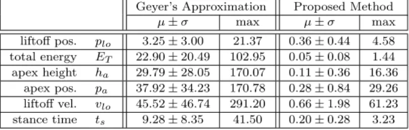
Table 2. Average percentage prediction errors for both Geyer’s and our methods in predicting various elements of the SLIP state.
Geyer’s Approximation Proposed Method
µ± σ max µ± σ max
liftoff pos. plo 3.25 ± 3.00 21.37 0.36 ± 0.44 4.58 total energy ET 22.90 ± 20.49 102.95 0.05 ± 0.08 1.44 apex height ha 29.79 ± 28.05 170.07 0.11 ± 0.36 16.36
apex pos. pa 37.92 ± 34.23 170.78 0.28 ± 0.84 29.26 liftoff vel. vlo 45.52 ± 46.74 291.20 0.66 ± 1.98 61.23 stance time ts 9.28 ± 8.35 41.50 0.20 ± 0.28 3.23 0 0.1 0.2 0.3 0.4 0.5 0 20 40 60 80 100 120 140 Damping Ratio - ζ0 -% Error
Mean Apex Position Percentage Error vs. Damping Ratio Geyer’s Solution Proposed Solution 0 0.1 0.2 0.3 0.4 0.5 0 10 20 30 40 50 60 70 80 Damping Ratio - ζ0 -% Error
Mean Total Mechanical Energy Percentage Error vs. Damping Ratio Geyer’s Solution
Proposed Solution
Fig. 2. Left: Average apex position prediction performance as a function of damping. Right: Average total mechanical energy prediction performance as a function of damping. The vertical bars represent the corresponding standard deviation.
As shown in Table 2, the average predictive performance of our algo-rithm across the entire range of simulations is significantly better than that of Geyer’s method.10Similarly, Fig. 2 illustrates the consistency of our ap-proximations as a function of damping. Interestingly, our apap-proximations perform better on the average with increased damping, which is due to the decreased amount of time spent in the stance phase when the radial velocity is decreased with higher damping in the leg.
5.2. Tracking Performance under Gait Control
0 0.05 0.1 0.15 0.2 0.25 0.3 0 1 2 3 4 5 6 7 Damping Ratio − ζ0 − % Error
Mean Steady State Apex Speed Percentage Error vs. Damping Ratio Geyer’s Solution Proposed Solution 0 0.05 0.1 0.15 0.2 0.25 0.3 0 5 10 15 20 25 Damping Ratio − ζ0 − % Error
Mean Steady State Apex Height Percentage Error vs. Damping Ratio Geyer’s Solution
Proposed Solution
Fig. 3. Comparison of apex forward speed (left) and height (right) mean tracking errors at steady-state for a spring-mass runner with different damping coefficients in the leg.
In order to characterize the utility of our approximation method for the design of locomotion controllers, we compared the tracking performance of a deadbeat gait controller9 based on Geyer’s approximations and our new method. Simulations were done with m = 1 and l0= 1, covering ˙xa∈ [1, 4],
˙x∗
a ∈ [1, 4], ya ∈ [1.5, 1.8], ya∗∈ [1.5, 1.8], k ∈ [1000, 2000] and ζ0 ∈ [0, 0.3], where ˙x∗
a and y∗a denote the desired goal state.
Fig. 3 shows average steady state tracking errors for gait controllers based on Geyer’s approximations and our method in trying to stabilize lo-comotion around the desired apex speed and height. Our results show that in both apex states of the SLIP, the tracking performance of the controller based on our algorithm outperforms existing alternatives in the presence of damping. Even though the accuracy‘ of both controllers decreases with increased damping, Geyer’s map is much more sensitive to this parame-ter. The real difference between the controllers is seen in the apex height performance, which indicates the dominant effect of damping in the verti-cal dynamics. Overall, these results show that our analytic approximation provides a very accurate characterization of the SLIP stance dynamics for
physical robot platforms where the effects of damping cannot be ignored. 6. Conclusion
In this paper, we proposed an analytical approximation to the stance dy-namics of the Spring-Loaded Inverted Pendulum model that also takes into account non-negligible damping in the leg. Our simulation studies showed that both the predictive performance of our fully analytic approximations as well as the tracking performance of the resulting deadbeat controller significantly outperform existing approximation methods. We believe that such an accurate analytical stance map to the dynamics of the SLIP model will be invaluable in the design and analysis of physically realizable and effective controllers for dynamic legged locomotion.
References
1. R. M. Alexander, Three uses for springs in legged locomotion., International
Journal of Robotics Research 9, 53 (1990).
2. R. Blickhan and R. J. Full, Similarity in multilegged locomotion: Bouncing like a monopode, J. of Comp. Physiology A: Neuroethology, Sensory, Neural,
and Behavioral Phys. 173, 509(November 1993).
3. W. J. Schwind, Spring loaded inverted pendulum running: a plant model, PhD thesis, University of Michigan, (Ann Arbor, MI, USA, 1998).
4. M. H. Raibert, Legged robots that balance (MIT Pr., Cambridge, MA, 1986). 5. P. Gregorio, M. Ahmadi and M. Buehler, Design, Control, and Energetics of an Electrically Actuated Legged Robot, Transactions on Systems, Man, and
Cybernetics 27, 626(August 1997).
6. S. G. Carver, Control of a spring-mass hopper, PhD thesis, Cornell University, (Ithaca, NY, USA, 2003).
7. J. W. Hurst, J. Chestnutt and A. Rizzi, Design and philosophy of the Bi-MASC, a highly dynamic biped, in Proc. of the Int. Conf. On Robotics and
Automation, (Pittsburgh, PA, 2007).
8. G. Zeglin, The Bow Leg Hopping Robot, PhD thesis, Carnegie Mellon Uni-versity, (Pittsburgh, PA, USA, 1999).
9. U. Saranli, Dynamic locomotion with a hexapod robot, PhD thesis, Univer-sity of Michigan, (Ann Arbor, MI, USA, 2002).
10. H. Geyer, A. Seyfarth and R. Blickhan, Spring-mass running: simple approxi-mate solution and application to gait stability, Journal of Theoretical Biology
232, 315(Feb 2005).
11. O. Arslan, U. Saranlı and O. Morg¨ul, An aproximate stance map of the spring
mass hopper with gravity correction for nonsymmetric locomotions, in Proc.
of the Int. Conf. on Robotics and Automation, (Kobe, Japan, 2009). 12. W. J. Schwind and D. E. Koditschek, Approximating the Stance Map of a 2
DOF Monoped Runner, Journal of Nonlinear Science 10, 533 (2000).
View publication stats View publication stats