Sm®tLïTY.Or HOPFIfLS^
ASSOC
'^lORY ■ Α· υ і и в м ..l 'T t O . V O . Т Н £ ; 0 £ :Ρ Λ η Τ Μ £ Ν Τ ' V \V K V "'IE L 5 C T Ş 0 j\İİC 3 £ îV 3 jr \ 'J J 'j JO.j 0.^DESIGN AND STABILITY OF HOPFIELD
ASSOCIATIVE MEMORY
A THESIS
SUBMITTED TO THE DEPARTMENT OF ELECTRICAL AND ELECTRONICS ENGINEERING
AND THE INSTITUTE OF ENGINEERING AND SCIENCES OF BILKENT UNIVERSITY
IN PARTIAL FULFILLMENT OF THE REQUIREMENTS FOR THE DEGREE OF
MASTER OF SCIENCE
By
M. Erkan Savran
Ч :Т SZ S-
-?
11
I certify that I have read this thesis and that in my opinion it is fully adequate, in scope and in quality, as a thesis for the degree of Master of Science.
M - r f i / i ___ r MoTffiilfPrii
Assist. Prof. Dr. Ömer Motgiil(Principal Advisor)
I certify that I ha,ve read this thesis and that in my opinion it is fully adf^quate, in scope and in quality, as a thesis for the degree of Master of Science.
kkoX'^/Y\AJ)\
.Assoc. Prof. Dr. Mehmet ,A.li Tc i
I certify that I have read this thesis and that in my opinion it is fully adequate, in scope and in quality, as a thesis for the degree of Master of Science.
Assist. Prof. Dr. Kemal Oflazer
Approved for the Institute of Engineering and Sciences:
Prof. Dr. Mehmet
ABSTRACT
DESIGN AND STABILITY OF HOPFIELD ASSOCIATIVE
MEMORY
M. Erkan Savraii
M.S. in Electrical and Electronics Engineering
Supervisor: Assist. Prof. Dr. Ömer Morgiil
September 1991
This thesis is concerned with the selection of connection weights of Hopfielcl neural network model so that the network functions as a content addressable memory (CAM). We deal with both the discrete and the continuous-time ver sions of the model using hard-limiter and sigmoid type nonlinearities in the neuron outputs. The analysis can be emplo3^ed if any other invertible nonlinear ity is used. The general characterization of connection weights for fixed-point programming and a condition for asymptotic stability of these fixed points are presented. The general form of connection weights is then inserted in the con dition to obtain a design rule. The characterization procedure is also emploj'ed for discrete-time cellular neural networks.
Keywords: Hopfield neural network, content addressable memory, fixed- point programming, cellular neural networks.
ÖZET
HOPFIELD ÇAĞRIŞIMSAL BELLEK TASARIMI VE
KARARLILIĞI
M. Erkan Savran
Elektrik ve Elektronik Mühendisliği Bölümü Yüksek Lisans
Tez Yöneticisi: Yard. Doç. Dr. Ömer Morgül
Eylül 1991
Bu tez Hopfield sinirsel ağ modelinin içerik adreslenebilir bellek olarak çalı şabilmesi için bağlantı ağırlıklarının seçimi ile ilgilidir. Sinir çıktılarında sigmo id ve signum türü fonksiyonlar kullanılarak, modelin eşzamanlı yenileme kuralı ile çalışcin ayrık ve sürekli zaman halleri incelenmiştir. Analiz herhangi tersi o- lan bir fonksiyon kullanıldığında da uygulanabilir. Sabit nokta programlaması için bağlantı ağırlıklarının genel yapısı ve bir asimtotik kararlılık şartı verilmiş tir. Genel yapı daha sonra bu şarta konarak bir tasarım kuralı elde edilmiştir. Genel yapı prosedürü ayrık zamanlı hücresel sinir ağlarında da kullanılmıştır.
Anahtar Sözcükler: Hopfield sinirsel· ağı, içerik adreslenebilir bellek, sabit nokta programlaması, lıücresel sinir ağları.
To m y family,
ACKNOWLEDG.MENT
I am grateful to Assist. Prof. Ömer Morgül, for his supervision, guidance, encouragement ai. d patience during the development of this thesis. I am in debted to the members of the thesis committee: Assoc. Prof. Mehmet Ali Tan and Assist. Prof. Kemal Oilazer.
I want to thank to my family for their constant support and to all my friends, especially B. Fırat Kılıç, Atilla Malaş and Taner Oğuzer for their many valuable discussions.
C o n te n ts
1 Inti'ccluction 1
2 M athem atical Prelim inaries 3
2.1 Singular Value D ecom position... 3
2.2 Induced Matrix Norms and Jacobian of a Function 5 3 P ast Work on Hopfield M odel 8 4 A ssociative M em ory Design for a Class of N eural N ets 15 4.1 Content Addressable Memory and Hopfield M o d e l... 15
4.1.1 Content Addressable Memory (C A M )... 15
4.1.2 Hopfield M o d e l... 16
4.2 M otivation... 17
4.3 Discrete-Time C a s e ... 18
4.3.1 Outer Product Rule 27 4.4 Continuous-Time C a s e ... 28
4.5 Cellular Neural Networks... 33
5 Conclusion 37
L ist o f F ig u r e s
4.1 Hard-Limiter and Sigmoid functions... 17 4.2 Safe region for the eigenvalues of T G ... 31 4.3 Topology of a cellular neural n e tw o rk ... 33
C h a p te r 1
I n tr o d u c tio n
In recent years, the neural network model proposed by Hopfield has attracted a great deal of interest among researchers from various fields. This is due to a number of attractive features of these networks such as collective com putation capabilities, massively parallel processing, etc., and these properties could be used in areas like control & robotics, pattern recognition and content addressable memory (CAM) design.
The Hopfield model consists of neurons, which are multi-input, single output, nonlinear processing units, and a large number of interconnections between them. The model has a feedback structure so that each neuron can have information about the outputs of the other neurons. It is this high degree of connectivity that makes the neural networks computationally attractive. Hopfield has showed that with a proper choice of connection weights, the net work can perform well as a CAM or can be used in solving difficult optimization problems such as traveling salesman problem (TSP) [1], [3].
Many researchers have argued certain aspects of Hopfield neural network and proposed methods of cidjusting the connection weights lor specific tasks. For the associative memory design, still most of these methods suffer from sig nificant drawbacks, such as the existence of a large number of spurious memory vectors, or some conditions that should be posed on memory vectors so that they can be stored by those methods. In [2], Hopfield has used outer product rule, which is one of the most widely used methods, to store a given set of memory vectors. In [12] and [15], memory vectors have been chosen linearly independent and successfully stored. McEliece in [14], has proposed memory vectors to be eigenvectors of connection matrix with positive eigenvalues and Michel in [5], has synthesized the connection matrix so that the memory vec tors become the eigenvectors of that matrix with a single degenerate positive
CHAPTER 1. INTRODUCTION
eigenvalue (see also [8]). In [9], [10] and [11], Bruck and Goles have investigated the convergence properties of the network depending on the topology and the mode of operation (either serial or parallel). The work done by these people will be explained in detail in Chapter 3.
The subject of this thesis is to make a general characterization of all possible connection weights so that the network performs as an associative memory. A stability analysis is also done for a large class of Hopfield neural networks that contain functions having continuous first derivatives in their neuron outputs. The characterization process is then carried out to cellular neural networks proposed by Chua and Yang [20], which have important applications in areas such as image processing and pattern recognition. In cellular neural networks memory patterns are matrices rather than vectors and the topology is different since a certain node can communicate with a predefined neighborhood onl}^
In this study, we consider both discrete and continuous-time Hopfield neu ral networks with synchronous update rule and discrete-time cellular neural networks. We give a general characterization of all possible connection weights which store a given set of patterns into the neural net (i.e. each pattern becomes a fixed point of the network). We use several class of functions in the neurons and investigate the stability properties of the memory vectors for which the functions used in the neurons have continuous first derivatives. The analysis is supported by examples and some widely used methods are also discussed.
The thesis is organized as follows. In Chapter 2, we present the mathe matical tools employed in the study such as singular value decomposition and matrix norms. In Chapter 3, we summarize the past work on Hopfield model and present the material which have been most important for us. In Chapter 4, we define our design problem (together with the motivation for it) for the discrete-time case first and give solutions to the problem for the cases depend ing on the nonlinearity used in the neuron outputs. We then give some results about the stability of the equilibria when sigmoid type nonlinearity is used. We redefine the design problem for the continuous-time case, give solutions to the problem depending on the nonlinearity and provide results concerning the stability of the equilibria. Finally, the design process is used for cellular neural networks. In Chapter 5, we give concluding remarks.
C h a p te r 2
M a th e r a a tic a l P r e lim in a r ie s
2.1
Singular V alue D ec o m p o sitio n
This chapter will serve as an auxiliary one in which we are going to make defini tions and present some mathematical tools that will be used in the subsequent chapters.
Let A G since A ^A is a symmetric positive semidefinite matrix, it has n non-negative eigenvalues, cr^,. . . ,o·^, with n corresponding orthonormal eigenvectors, v i , . . . , v„. Assume that cr\ > ct2 > . . ■ > <Tr > 0] crj = 0, j =
r + 1 , .. . ,n. Obvious!}' r = rank{A) and we have
A^Av,· = erf Vi, i = 1, . . . , n (2.1) Note that, Vr+i,. . . , v„, belong to the nullspace of A, they are orthonormal and arbitrary otherwise. We define the vectors u, as follows:
Av,- = (T,u,·, f =
It is easy to see that the vectors u,· are orthonormal:
(2.2)
ufu} = ——(A v,yA v} = — v f y j : = 1, . . . ,r
0" i 0 j 01 (2.3)
Let u,-,i = r -f denote an arbitrary orthonormal complement of the vectors Uj-,f = 1,...,? ·, defined by (2.3). Define U = [ u i...u „ ,] ,S =
)
, with D = diag(ai,. . . , cr,.), and V = [ v i... v,,]. Then, it is easy to see that we have the following decomposition
CHAPTER 2. MATHEMATICAL PRELIMINARIES
A = U E V ^ (2.4)
To summarize, we have the following theorem; square brackets denote the complex case [23].
Theorem 1: Let A G Then there exist orthogonal [unitary] matrices U G 3?™^^ [Cmxmj y ^ gj.nxn
A = USV^' [U SV ^] (2.5)
where and denote the transpose and conjugate transpose of V, respec tively, and
S =
V
D 0
0 0
J
D = diag(ai, . . . , cr^) with cti > 0-2 > ... > cr,· > 0, where r = rank{A)
Proof: See [23].
The numbers a i , . .. ,ar together with <7^+1 = 0 , . . . , (7„ = 0 are called the singular values of A and they are the positive square roots of the eigenvalues (which are non-negative) of A ^A [A-^^A], The columns of U are called the left singular vectors of A (the orthonormal eigenvectors of AA^" [AA^^]) while the columns of V are called the right singular vectors of A (the orthonormal eigenvectors of A ^A [A^A]). The matrix A^' [A^] has m singular values, the positive square roots of the eigenvalues of AA^ [AA·^^]. The r (=rank (A)) nonzero singular values of A and A^ [A·^] are, of course, the same. The choice of A ^A [A-^^A] rather than A A ^ [AA^^] in the definition of singular values is arbitrary.
It is not generally a good idea to compute the singular viilues of A by first finding the eigenvalues of A^A. As in the case of linear least squares problems, the computation of A^ A involves unnecessary numerical inaccuracy. For example, let
A =
/1 l \
¡1 0 VO
CHAPTER 2. MATHEMATICAL PRELIMINARIES then / J A = 1 + 13^ 1 1 l +/?2 so that c 7ı(A ) = (2 + ^ ^ ) ^ a,{A ) = \^\.
If < 6o, the machine precision, the computed A ^A hcis the form and one obtains from diagonalization d'i(A) = \/2, <J2(A) = 0.
1 1
1 1
Fortunately, Golub and Reinsch [22] have developed an extremel}'^ efficient and stable algorithm for computing the SVD which does not suffer from the above defect. Golub and Reinsch employs Householder transformations to reduce A to bidiagonal form, and then the QR algorithm to find the singular values of the bidiagonal matrix. These two phases properly combined produce the singular value decomposition of A.
B}'· using Householder transformations, the mcitrix A is first transformed into a matrix having the same singular values as A, i.e. if the SVD of A is A = U S V ^ , that of is matrix, which is in bidiagonal form, is then iteratively diagonalized using a variant of QR algorithm so that
For details, see [22].
2.2
In d u ced M atrix N orm s and Jacobian o f a F u nction
Definition: Let ||.|| be a given norm on G”. Then for each matrix A € 6'"^", the quantity ||A||· defined by
||A||,. = sup = sup IIAxil = sup ||Ax|| (2.6)
xyio,xeC’"X’> ll^ ll ||x||=i l|x||<i
is called the induced (matrix) norm of A corresponding to the vector norm ||.| (17)·
CHAPTER 2. MATHEMATICAL PRELIMINARIES
It should be noted that there are two distinct functions involved in definition (2.6): One is the norm function ||.|| mapping C ” into and the other is the norm function ||.||j· mapping (7"^" into
The induced norm of a matrix A (or the induced norm of a linear mapping A) can be given a simple geometric interpretation. Equation (2.6) shows that ||A|||· is the least upper bound of the ratio ||A x ||/||x || as x varies over C^. In this sense, ||A||j· can be thought of as the maximum ’’gain” of the mapping A.
The induced norms have the special feature that they are submultiplicative; i.e.
ЦАВ11, < ||A ||.||B ||. V A .B e C “ ” Another useful identity is
(2.7)
IIA + B||.. < ||A||,. + ||B||, VA,B € (2.8) The induced matrix norms corresponding to the vector norms ||.||^ , ||.|li, and
гПз respectively, are known and are displa.yed below.
0 Halloo = ll-^llico = l«<il {max.rowswn)
it) ||x||j = llAllii = m a x 5 ^ | a ij I (m ax. col и m nsu m )
>») ||x||, = (У ^ ||A ||„ = (A „.,(A "A )|^ = <7,„ ,(A ) i
where Xmax{A.^^·^) =maximum eigenvalue of A ^A . Similarly ||A “’ |
1/
^min(A).¡2
Lastly, we define the Jacobian of a vector function. Let f(x) : 3?” —> 3?”^ be a differentiable vector function.
/ . q \
X = >f(x) =
V "■“ /
/
M^) \
CHAPTER 2. MATHEMATICAL PRELIMINARIES
The Jacobian dijd'x.: —i· is defined as:
d i
( 2Ad x i 2 L · \
dxn d x ~
C h a p te r 3
P a s t W ork o n H o p fie ld M o d e l
In 1982, Hopfield proposed a system, based on biological nervous systems, which performs as an associative memory. He has called the processing devices ’’neurons” and each neuron i had two states: either V, = 0 (’’not firing”) or Vi = 1 (’’firing at maximum rate”).
In Hopfield model, each neuron i has a connection made to it from neuron j, the strength of connection is defined as Tij. The instantaneous state of the system is specified by listing the N values of so it is represented by a binaiy word of N bits. In general, the next state of the network is computed from the current states at a subset of the nodes of the network, to be denoted by S [9]. The modes of operation are determined by the method by which the set S is selected in each tim.e interval. If the computation is performed at a single node in any time interval that is, ji'l = 1 (|S'| denoting the number of nodes in the set S) then the network is operating in full}'^ as5mchronous mode or serial mode and if the computation is performed in all nodes in the same that is, l^l = N (N is the total number of nodes in the netw ork), then the network is said to be operating in sjmchronous mode or fully parallel mode. All the other cases, that is, 1 < I*?! < N, will be called asynchronous or parallel modes of operation. The set S can be chosen randomly or according to some deterministic rule.
In Hopfield model, each neui'on i readjusts its state randomly in time, set ting
CHAPTER 3. PAST WORK ON HOPFIELD MODEL
Vi -> 0 if ^ TijVj < 0
Thus each neuron randomly and asynchronously evaluates whether it is above or below 0 and readjusts accordingly.
Associative memory problem is to store a given set of states to the network, i.e. states should be fixed points of the network. For the associative memory problem, Hopfield has suggested the rule to store the set of states F®, s =
Tii = J ^ ( 2 V ; · - m v ; - 1) (3.1) but with Tii = 0. This model has stable limit points. Hopfield considers the special case Tij = Tji, and defines
(3.2)
A E due to AVi is given by
A E = - A V i Y ^ T i j V (3.3) j¥=i
Thus, the algorithm for altering V causes E to be monotonically decreasing function. State changes will continue until a minimum (local) E is reached.
Apart from the discrete stochastic model above, Hopfield has also proposed a continuous deterministic model for the associative memory problem based on continuous variables yet keeping all the significant beha\'iour of the original discrete model. He has constructed an electronic model using Ccipacitors, re sistors and amplifiers each of which represented a certciin element of the nerve system.
The equation governing the electronic circuit is nonlinear and is given as follows
CHAPTER 3. PAST WORK ON HOPFIELD MODEL 10
where u,· is the input to nonlinear amplifier, gi{uj) represents the input-output characteristics of the nonlinear amplifier, C',·, Ri represent the capacitor and resistor respectively, and /,· is any other fixed input current.
Hopfield again employs a Lyapunov (or energy) function approach to in vestigate the stability properties of the network. He chooses the Lyapunov function as
® = f ' s7'{V)dV
t j i i
Its time derivative for a symmetric T is
dE idt = - J 2 d V i/d t(Y ^ TijVj - Ui/Ri -j- /,·)
i j
The parenthesis is the right-hand side of (3.4), so
(3.6)
dE/dt = ~ Y Ci(d(g-'(Vi))JdV,)(dVi/dtf (3.7)
Since g- ^{Vi) is a monotone increasing function and Ci is positive, each term in this sum is nonnegative. Therefore dE/dt < 0, and by LaSalle’s theorem
dE/dt = 0 ^ dVi/dt = 0 for all i.
Together with the boundedness of E, equation above shows that the time evo lution of the system is a motion in state-space that seeks out miirima in E and comes to a stop at such points. However, there is no guarantee that the network will find the best minimum.
In [l], Hopfield has also investigated the relation between the stable states of his two models. He has concluded that the only stable points of the extremely high gain continuous deterministic system corresponds to the stable points of the stochastic system.
Manj7 scientists have made research on diflerent aspects and appliccitions of Hopfield model such as content addressable memory (CAM), some optimization problems, and capacity of the model. Here, a few of them will be explained but according to me, they are the most suitable ones to mention here.
CHAPTER 3. PAST WORK ON HOPFIELD MODEL 11
A. Michel in his several papers has analyzed a certain class of nonlinear, autonomous, differential and difference equations containing the models of Hop- field. He deals with differential equations of the form (see [6])
clyi
— = F(x) = A x -f TS(x) -I-1
at
(3.8)
where x = (a)i,. . . , G F : is a measurable function, A = diag{—pi, . . . , —pn) is an n x n constant matrix with p, > 0, T = [Tij] is an n X n constant matrix, I = ( / i , . . . , 7,-,)^ is a constant vector and S :
is a measurable function defined by S(x) = ·. g{,^) beir.g a monotonically nondecreasing, continuously differentiable functicm with p(0) 0 and |p(a;)| < 1 . His difference equations are in the form of (see [7])
u(7 + 1) = Tg(u(A·)) + Au(yt) + I (3.9)
where T = [Tij] G A = diagiA,:,) G I = [/,■] G 3?”, and g =
[pi,. . . ,p„]^ : Pi’s being monotonically nondecreasing, continuously differentiable function with gi{0) = 0 and |pi:(a;)| < 1.
For both of the differential and difference equations, some conditions are imposed on T and A matrices so that an appropriate analysis can be done. In the analysis, Michel develops the solutions of the systems, makes the concept of equilibrium point precise, gives bounds on the number of asymptotically sta ble equilibrium points and discusses the distribution of the equilibrium points in the state-space. He also constructs an energy function to investigate the stability properties of the equilibrium points.
For the synthesis procedure, he defines the set as = {x G — 1 < a;,· < 1, f = 1, . . . , ?7.}. Given m vectors in .B”, say Qq,. . . , am, it is desired to design T , I (for the system (3.8) or (3.9)) such that
1) a i , . . . , am are stable output vectors of the system. 2) The system has no periodic output sequences.
3) The total number of stable output vectors of the system in the set /7" — {q i, . . . , a'm} is as small as possible.
4) The domain of attraction of each Oj is as large as possible.
Here as an example, we give Michel’s synthesis procedure, which fulfills the design objectives stated above, for the continuous-time system
CHAPTER 3. PAST WORK ON HOPFIELD MODEL 12
Ч
^ = - x + T S (x )+ I (3.10)
where S is the function defined in (3.8). Suppose we are given m vectors Q'l,. . . , dm in jB" which are to be stored as stable otuput vectors for (3.10).
We proceed as follows:
1) Compute the n x (m — 1) matrix
Y = [o-i - cKin,.. ., a'm-l - o;m]
2) Perform a singular value decomposition of Y and obtain the matrices U, V and S such that Y = U S V ^ , where U and V are unitary matrice.s and where S is a diagonal matrix with the singular values of Y on its diagonal (this can be accomplished by standard computer routines). Let Y = [ y i,. . . , ym -i], U = [ u i ,. . . , Un] and k ^dimension of S p an (y i,. . . , ym -i)· From the proper ties of singular value decomposition, we know that k =rank of S , { u i, . . . , u^} is an orthonormal basis of S p a n (y i,... ,ym _i) and { u i , . . . , Uu} is an orthonor mal basis of
3) Compute
= 1^.71 = E “ ‘“ t
¿=1 I=A:H-1
4) Choose a value for the parameter r > — 1 cind compute
T t = T"*" — tT , It = cvin ~ FrCi'in
In particular, the optinicil pair {Top,!^^} is given by
-op T"*” TopX , Xp — Cim ~
where Top — 7nin{T^^/T^i , ! < « < « } .
Michel’s work is essentially on analysis and design of Hopfield t}q3e systems. Bruck and Coles deal with rather a different aspect of Hopfield model using energy (Lyapunov) functions and a graph theoretic approach. They show that the known convergence properties of the Hopfield model can be reduced to a very simple case and the fully parallel mode of operation is a special case of the
CHAPTER 3. PAST WORK ON HOPFIELD MODEL 13
serial mode of operation. We begin presenting their work by some definitions and notation.
The order of the Hopfield network is the number of nodes in the correspond ing weighted graph (by a weighted graph, we mean a set of nodes together with a set of weighted branches with the condition that each branch terminates at each end into a node). Let N be a neural network of order n; then N is uniquely defined by (T,i*) where:
•T is an n X n matrix, with element t{j equal to the weight attached to
edge (i, j).
•i^ is a vector of dimension n, where element i^· denotes the threshold at tached to node i.
Every node (neuron) can be in one of two possible states, either 1 or -1. The state of node i at time t is denoted by The state of the neural network at time t is the vector V (i) = (yi(i)) · · · )^’n(^))· The state of a node at time (i + 1) is computed by
•ji{t + 1) = Sign{Hi{t)) = S i ( j n { ^ - i\) =
i=l
1 i f i i , ( i ) > 0 — 1 otherwise A set of distinct states { V i,. . . , Vk} is a cycle of length k if a sequence of eval uations results in the sequence of states: V i , . . . , Vr-, V i , ... repeating forever.
The main contribution of Bruck and Goles [9] is the following theorem. Theorem 2: Let N = (T,!*") be a neural network. Then the following hold: i) If N is operating in a serial mode and T is a symmetric matrix with zero diagonal, then the network will alwaj'^s converge to a stable state.
ii) If N is operating in a serial mode and T is a symmetric matrix with nonnegative elements on the diagonal, then the network will always converge to a stable state.
iii) If N is operating in a fully parallel mode then, for an arbitrary symmetric matrix T , the network will always converge to a stable state or a cycle of length 2; that is, the cycles in the state-space are length < 2.
iv) If N is operating in a fully parallel mode then, for an antisymmetric matrix T with zero diagonal, with i*” = 0, the network will always converge to a cycle of length 4.
CHAPTER 3. PAST WORK ON HOPFIELD MODEL 14
Other subjects about content addressabilitj^ and Hopfield model that are studied by Abu-Mostafa [13], McEliece [14], Venkatesh [12] and Dembo [15] are the capacity of Hopfield model and alternative construction schemes of connection weight matrices for content addressabilitj'.
Venkatesh and Dembo [15] have chosen the memory vectors linearly in dependent in order to store them successfully by their construction scheme. McEliece [14] has proposed memory vectors be eigenvectors of connection weight matrix with positive eigenvalues. These schemes guarantee the stor age of memory vectors as fixed points.
Although different definitions exist for the capacity of a neural network, generally we may define the capacity as the maximum number K such that any K vectors of N entries can be made stable in a network of N neurons by the proper choice of connection weight matrix and the threshold vector attached to the neurons.
For the above definition, Abu-Mostafa [13] has shown that the capacity of Hopfield model (using hard-limiter functions in the neurons) is n for an n neuron network.
Using an alternative approach to capacity, McEliece [14] has shown that the capacity of a Hopfield neural associative memory of n neurons with sum- of-outer product interconnections is m = nf 2logn if we are willing to give up being able to remember a small fraction of the m memories, and m = n/A log n if all memories must be remembered.
C h a p te r 4
A s s o c ia tiv e M e m o r y D e s ig n for a C la ss o f
N e u r a l N e t s
4.1
C on ten t A d d ressab le M em ory and H opfield M o d el
In this section, we give brief information about content addressable memories and Hopfield neural networks.
4.1.1
C on ten t A d d ressa b le M em ory (C A M )
Human brain has an associative proiDerty that when a reasonable partial in formation of a vast set of incidents is supplied, the huge set of information is automatically invoked or synthesized. It has been observed that highly in terconnected neural networks have this collective property known as CAM in literature [19]. This property arises from the fact that the motion of a sys tem has stcible points in state-space which can be thought of as a kind of memory. From an initial state which contains partial information cibout a par ticular memory (i.e. a stable state), the system asymptotically converges to that memory. The memory is reached b}^ knowing its partial content rather than its address, hence called CAM.
Convergent flow to stored memory vectors (i.e. stable states) is the essential feciture of this CAM operation. For normal operation of CAM, the memory items should have reasonable regions of attraction, sq beginning from any initial
point within the region of attraction of a particular item, we should be able to reach that item. Therefore, while designing a content addressable memory, one should take into account the asymptotic stabilities of memory items. The items
CHAPTER 4. ASSOCIATIVE MEMORY DESIGN FOR A CLASS OF NEURAL NETS16
which are much alike, like the photographs of twins, may cause problems in the separation of regions of attraction, i.e. their stable storage in the memory. The existence of spurious items is another fact that should be eliminated as much as possible. Sometimes, the CAM operation converges to a memory which does not belong to the set of memory patterns stored beforehand. These spurious patterns are generally the linear combinations and complements of stored patterns.
The main approach of Hopfield and many others for the convergence prop erties to stable states is to define a so called energy function and to show that this energy function is nondecreasing when the state of the network changes. Since the energy function is bounded from above, it follows that it will con verge to some value. In other words, memory vectors or the states to which the network converges are local minima of this energy function. This means that the networks are performing optimization of a well defined fuirction. Un fortunately, there is no guarantee that the network will find the best minimum. Initial states, which are queries to memory vectors, contain only partial or erro neous information about memory vectors. And the network through iteration simply finds the minimum that best fits the query.
In this thesis, 'we will not employ a Lyapunov or energy function approach to investigate the design and stability properties of Hopfield neural networks but rather use more direct methods.
4.1.2
H opfield M od el
Hopfield network is constructed by connecting a large number of simple pro cessing units to each other by links having fixed weights. These weights are modeled cifter the synaptic connections between the real neurons. The pro cessing units stand for the real neurons where each one of them is a nonlinear function chosen to be a monotonously increasing and usually continuous func tion of its arguments.
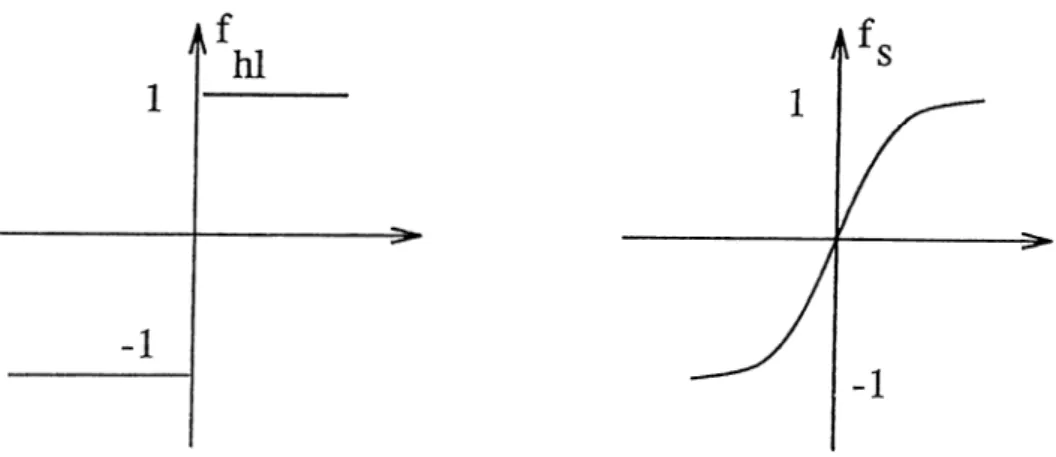
Each neuron has a current state (or input) and an output. It has feedback connections from the outputs of all the other neurons as well as itself and its current state is a weighted sum of all the outputs of the previous instant. This current state is processed by the neuron i.e. mathematically, undergoes a nonlinear function and the value of the function is simply the output of the neuron. The function in the neuron is usually the hard-limiter function or a sigmoid type nonlinearity as shown in Fig. 4.1.
CHAPTER 4. ASSOCIATIVE MEMORY DESIGN FOR A CLASS OF NEURAL NETSll
Figure 4.1: Hard-Limiter and Sigmoid functions
The output of the neuron is fed to the input of the neuron by a connection weight Uj. Therefore the output of the neuron is first multiplied by tij and then fed back to the input of the P’’· one and the total input of the neuron is the summation over all feedbacks from the other neurons including itself. In addition each neuron has an offset bias of fed to its input.
Hopfield model has two versions: i) Discrete-time
ii) Continuous-time
In discrete-time version, the outputs of the neurons are updated at discrete time instants whereas in continuous-time, they are updated continuously. We use synchronous update rule for both of the versions in this paper.
4.2
M o tiv a tio n
Although Hopfield model and its content addressability have been studied be fore, the main motivation for this study has been the lack of e.x:istence of a general associative memory design and the conditions to check the quality of the design.
We begin with asking some questioirs:
1) What are the necessar}'^ and sufficient conditions on T such that for the discrete-time model (using hard-limiter functions in neurons), all possible 2 ^ binary vectors of dimension N are the fixed points of T?
CHAPTER 4. ASSOCIATIVE MEMORY DESIGN FOR A CLASS OF NE URAL NETS18
T matrices which store this set. For a specific T, what can be said about the stability of memory vectors?
3) Apply the second question to the continuous-time case.
4) In discrete-time model, instead of hard-limiter function, use sigmoid type nonlinearities and apply the questions 1 and 2.
Above questions will be the subject of the subsequent sections.
4.3 D iscr ete-T im e Case
Let’s denote the outputs of the neurons by the vector x, the connection weights by the m atrix T , cind the offset biases by the vector i*", i.e. for an N neuron
network T is an TVx A'^ matrix with real comiDonents tij {tij being the connection weight from the output of neuron to the input of neuron), x is a real n.vector with components Xi (.Ti. being the output of neuron) and i*“ is a real n.vector with components i*’ (z,· being the offset bias of neuron). Let /( .) : be a function and let v € 3?"· be a vector. By f(v), it is meant that f is applied to all of the entries of v.
Then the dynamics of the discrete-time network is described by the follow ing difference equation
Xn+i = /(T x „ -t- i*”) (4.1)
where f(.) is a sigmoid type nonlinearity or signum function. The aim is to determine T and for the particular choice of appliccition.
Here we deal with discrete-time synchronous Hopfield model without the threshold vector i.e.
Xn+i = /(T x „ ) (4.2) where x G 3?·^, T € (i.e. the number of the neurons in the network is N). Before defining the design problem, the first question, in the previous section, is solved.
Theorem 3: All 2^ binary vectors of dimension N are the fixed points of (4.2), where / is the hard-limiter (signum) function, if and only if T (connection
CHAPTER 4. ASSOCIATWE MEMORY DESIGN FOR A CLASS OF NEURAL NETS19
weight matrix) satisfies the following row dominancy condition:
N
Li > ^ ] I^ijI ) 2 — 1, . . . , yV
i=l
Proof: To be a fixed point, a binary vector must stay in the same quad rant after it is multiplied by T. For row of T (i — the max imum of (where Xj is 1 or -1) is |iij| (since all 2^ binary vectors are considered, this maximum is achieved for each row) and Xi = sign(Y^^_^ Xjtij) iff the above row dominancy condition is satisfied. So. to store all 2^ binary vectors, T should satisfy
N
tii ^ ^ ^ \^ij \ ■) * — 1, . . . ,
i=lo¥«'
If /(.) : is a sigmoid type nonlinearit}'·, it is defined as
1 —
e~^~
= T T ^
where ^ > 0, /? € 5P. VVe consider the following problem.
(4.3)
Design problem: Given a set of vectors M. — { n ii,. . . , niA/}, m , G (—1,1)^'^, i = 1, . . . , M, find, if possible, all matrices T which store M into the network (i.e. for i — 1 ,... ,M ; m,· becomes a fixed point of (4.2) where / is given in (4.3)).
This problem is referred to as fixed-point programming and has been in vestigated for similar nonlinearities by several researchers, see [2], [4], [5], [12], [15]. The most famous one of these schemes is the outer product rule
M
T = m u n f (4.4)
1=1
which poses some conditions on the memory vectors to be stored. We’ll analyze the outer product rule and derive these conditions in section 3.
The solutions found in the literature to the design problem posed above are special solutions, and a characterization of all matrices T solving the problem stated above has not yet been given.
CHAPTER 4. ASSOCIATH^E MEMORY DESIGN FORA CLASS OF NEURAL NETS20
Let the number of the neurons in the network be N and let A4 = { n ii,. . . , itim}
be the set of vectors we want to store as fixed points. Placing them in columns of a matrix, it is obtained A = [niim 2 . . . ni^i] where A G Then the T matrix should satisfy the following equation
TA = f - \ A ) where / “ ^(A) G is defined as:
(4.5)
1/ '(A.)],·, = / ‘(aij) = 1 , . . . , M
( i.e. /~^(·) : (—1,1) —> is applied to all of the entries of the matrix A). Since f is given by (4.3), f~^ is defined as
Applying a singular value decomposition to A as follows
(4.6)
A = U S V ^ (4.7)
where U G S G , Y G U and V are unitary matrices and S is a block-diagonal matrix containing the singular values of A. Partitioning U, S and as
(4.8)
D = diag{ai,... ,cr,.), cxi > ct2 > · · · > cr,. > 0, ct,:’s are the singular
values of A.
Then, combining (4.7) & (4.8) and putting in (4.5) will yield
T U a = / - '( A ) V i D - i (4.9)
In order to find the rncitrices T which satisfy (4.9), Ui is conccitenated with U 2, which results in the following equation:
^ D 0 ^ v f ^
U = [U iU 2] ,S =
U V y v r j
b(A), Ui G U 2 G D G V
CHAPTER 4. ASSOCIATIVE MEMORY DESIGN FOR A CLASS OF NEURAL NETS21
Here U ' is any real N x (A^ — r) matrix. Hence it is obtained
T = /- ^ ( A ) V iD - ^ u f + u 'u : (4.11) The Eq. (4.11) characterizes all possible solutions of the design problem stated in this section. It is obvious that, with this choice of T , the vectors m,·,
1 = 1 , . . . , M, become fixed points of (4.2), but the stability of these equilibria
is not guaranteed a priori.
Stability: For the Hopfield model to function as a CAM, obviously it must be able to recover an original memory vector when ¡^resented with a probe vector close to it (usually in terms of Hamming distance). If the probe vector is considered as a corrupted version of the original memorj'^ vector, then it is possible to view the network’s operation as a form of error correction. There fore, each memory vector should be an asymptotically stable equilibrium point of (4.2). Hence each of these memory vectors will have a certain region of attraction, so that any probe vector in that region of attraction will converge to the memory vector.
To determine the stability of the fixed points, we make use of the following theorem.
Theorem 4: Consider the following system
X„+1 = f(x„) (4.12)
where f : 3?^ is a differentiable function. Let Xg be an equilibrium of this system (i.e. f(xe) = Xe)· If all the eigenvalues of dijdyi at x = Xg are inside the unit disc (i.e. less than 1 in norm), then the equilibrium point Xg of (4.12) is asymptotically stable.
Proof: See [16].
The following corollary easily follows from Theorem 1: Corollary 1: Let Xg be an equilibrium of (4.2). Let
F = 5//5x|x_y_i(x^) , where d f f d x is the Jacobian given by d f f d x = diag{df j d x i , .. . , d f Idx^ ).
If all the eigenvalues of F T are inside the unit disc, then Xg is an asymp totically stable equilibrium point.
CHAPTER 4. ASSOCIATIVE MEMORY DESIGN FOR A CLASS OF NEURAL NETS22
Proof: See Theorem 4 and (4.2).
To make use of the corollary 1 in the stability analysis, we need the following theorem:
Theorem 5: For an}/^ N x comple.x matrix M, we have the following interlacing property
o-mm(M) < |A,„,„(M)| < |A„,ax(M)| < (4.13) where amux the minimum and maxiiiium singular values of M, re spectively, and X-min, Xmax ^I'e the minimum and maximum eigenvalues of M , in absolute value, respectively. We note that amin = -yA„itn(M^M), ^max ^J~xm ax ( M . T M ) .
Proof: See [18].
As a result,we can write
|A^ax(FT)| <
a r r ^ a x i F T )= ||FT
||2< IIFII
2IITII
2= A„,„,(F)cr,„„,(T) (4.14)
where ||A ||2 denotes induced 2-norm of the matrix A, and ||A ||2 = cTmariA). (see [17]).
If we choose
.(T )<
1(4.15)
Amax(F)
then the as3m'iptotic stability of the equilibrium Xg is guaranteed. Of course, this condition is only a sufEcient condition which guarantees the asymptotic stability.
The above condition holds for a single memory vector. Thus, we should generalize for a set of memory vectors. For M. = { m i , . . . , mA/}, let F,· =
i = 1, · · ·, and
A/nax(F) — max A„,(12,(Fi)
(4.16)
CHAPTER 4. ASSOCIATIVE MEMORY DESIGN FOR A CLASS OF NEURAL NETS23
.(T )< (4.17)
■^max(F)
Since T = [/- i( A ) V iD - i U']U^, cr„,,(T ) < ||[/-i(A )V :D -^ is unitary, thus ||U ^||2 = 1. Also
cr„^ax(T) < ||[/-^ (A )V iD -i U ']||2 < ||/ - '( A ) ViD -^||2 + ||U '||2 (4.18) Hence if we can choose U' as
liu'lb < 1 ||/- ■ ( A ) V ,D - İ 2 (4.19) '^max(F)
then we guarantee the asymptotic stability of the memory vectors. For the ex istence of U', the right side of the above inequality should be non-negative. As the relationship between l/\m ax{F) and | | / “ ^(A )V iD “^||2 is highlj^ nonlinear, it needs further investigation.
Remark 1: To increase the bound on (Tmox(T), one should decrease A„iai(F), which in turn means one should choose equilibrium points where the slope is small on the sigmoid, i.e. near the asymptotes 1 & -1 (provided a U' exists for (4.19)).
We note that the same design procedure can be applied if the nonlinearity used in (4.2) is different than the sigmoid type. For example, consider the design problem for the following system:
x„,+i = sign{Txn) (4.20)
where x G 3?^, T € and the signum function is defined as:
sign{u) : u > 0
— 1 u < 0 (4.21)
Let { m i,. . . , niyv/} be a set of binary vectors to be stored in the neural network given by (4.20). As before, we set A = [m ini2... niM·]. Then the T matrix should satisfy:
TA = P Here P G and should satisfy
1) sign(aij) = sign(pij) i = 1 ,... ,N ■, j - I , ... ,M 2) Row space of A spans the row space of P.
Applying the singular value decomposition to A
A = U S V ^ (4.23)
where U € S G G U and V are unitary matrices and
S is a block-diagonal miitrix containing the singular values of A. Partitioning U, S and as
CHAPTER 4. ASSOCIATIVE MEMORY DESIGN FOR A CLASS OF NEURAL NETS24
/ D
0\
U = [ U i U 2] ,S =
V
0 0J
(4.24)
where r = ra7ik{A), Ui G U 2 G D G 3^’'^", V f G
Y2 € >:■'''·'', D = diag{ai,... ,ar). ai > a2 > ■ ■ ■ > CTr > 0, a^s are the
singular values of A. Applying the same steps in the preceding analj'^sis, it is obtained
T = P V iD - 'U f + U 'U (4.25)
where U' is any real N x (yV — r) matrix. The Eq. (4.25) characterizes all possible solutions of the design problem for the signum type nonlinearity. Note that
P
should satisfy the above conditions and U' is arbitrary. A particular choice isP
— TiA and U ' = —T2U 2, where ti and r2 are arbitrary positive constants. This choice yieldsT = riU iU ^ — T2U2U2
which is the form ofT
given in [5]. Observe thatP
= tiA means all the memory vectors areeigenvectors of
T
with a single positive eigenvalue ti (see Eq. (4.22)).In the analysis above, the threshold vector i*" is not used. Now, i*" will be inserted into the model to see whether it can be used as a control to reduce the number of spurious memory vectors. With i^, the model becomes
x„+i = sign{Txn + i'’) (4.26)
Now the question is: given
T,
the memory vectors j\4 = { n ij,. . . , iTiyv/} and the spurious memory vectors S = { s i,.. ..S5}, can i*" used to reduce the number of spurious memory vectors without disturbing the memory vectors?CHAPTER 4. ASSOCIATIVE MEMORY DESIGN FOR A CLASS OF NEURAL NETS25
We have a simple routine for the solution of this problem: memory vectors are put in columns of a matrix A, and spurious memory vectors in columns of a matrix B. Then A = [ m i m j .. . niA/], B = [siS2... ss] T[A|B] P n P l 2 P21 P22 P l M P 2M rxi T21 r\s T2S \ Pm PN2 ■ ■ · Pnm .. ■ VMS
The basic idea of the routine is to give the maximum sign change to the entries of the rows of T B by using i*" without changing the signs of the entries of T A .
For each row do the following:
i) Find the minimum absolute valued one of the positive elements of Pty’s
ii) Find the minimum absolute valued one of the negative elements of p,y’s
iii) For the positive elements of {j = 1, . . . , ,5’), find the number of ones which are smaller in absolute value than the minimum found in part i.
iv) For the negative elements of rif's {j — 1 . . . . , find the number of ones which are smaller in absolute value than the minimum found in part ii.
v) Take the maximum of the numbers found in part iii and part iv:
vl. if part iii is larger than part iv, choose i'· < 0 and choose it so that \Pim+\ > btl > b’u'il · · · > whei'e pimJr is the minimum absolute valued of positive p.j’s and r ,j i,... , are the positive ones of r,j’s which are smaller in absolute value than pim+ ·
v2. if part iv is larger than part iii, choose i\ > 0 and choose it so that
\ p i m - \ > lb'I > h’l'iil · · · > where is the minimum absolute valued of negative pij's and are the negative ones of ?-j-/s which are smaller in absolute value than pim- ■
CHAPTER 4. ASSOCIATIVE MEMORYDESIGN FOR A CLASS OF NEURAL NETS26 m i = Si / l \ 1 1
V I /
i \ 1 - 1 1/
/ l \ 1 1 V - 1 / , m 2 = , S2 = , S3 = 1 \ - 1 1 1/
(
1 \
1 - 1 V - 1 /be the memory vectors and
S4 —
/ - 1 \
1
1
v - 1 /
be the spurious ones.
Using the singular value decomposition techniques, T is chosen as
/
T = 0.8 -0.35 -0 .3 \ -0.225 Without the threshold vector i^:0.5 0.0167 0.45 \ 1.45 0.0167 0.25 -0.25 1.3167 - 0.2
0.1 -0.35 1.625 )
ri = (—1 1 1 1)^ is converging to Si, and r 2 = (1 — 1 1 — 1)^ is converging to - m i . Now A = 1 - 1 - 1 1 , B = / 1 1 1 - 1 \ 1 1 . 1 1 1 1 - 1 1 V I 1 / { 1 - 1 - 1 - i j T(A|B) 1.73 0.76 1.76 0.86 0.83 -0.73 \ 1.33 -1.53 1.36 0.86 0.83 1.56 -2.06 1.06 0.56 0.96 - 1.66 1.56 1.85 0.95 1.15 - 2.1 -1.4 -1.65 /
1) For the first row, minimum is 0.76, all the positive elements are greater than 0.76 on the right. So = 0.
2) For 1.33, 0.86 k 0.83 are smaller. For -1.53, there are no negative elements on the right. So choose ¿2 < 0 and 1.33 > > 0.86 > 0.83.
3) For the third row -2.06 is greater in absolute value than -1. 1.06 is greater than 0.56 L· 0.96. Thus choose 4 < 0 and 1.06 > |4 | > 0.96 > 0.56. 4 = —1.
4) For the fourth row, minimum is 0.95, but the only positive element 1.15 on the right is greater than 0.95. So 4 = 0. i*’ becomes = (0 - 1 - 1 0)^.
With the threshold vector i*", the network becomes
Xn+i = Sign{T:Kn + 4)
ri = (—1 1 1 1)^ and Si = (1 1 1 1)^ is now converging to m j. As a result, with the insertion of a proper i*, it is achieved to reduce the number of spurious memory vectors and also enlarge the region of attraction of memory vectors.
CHAPTER 4. ASSOCIATIVE MEMORY DESIGN FOR A CLASS OF NEURAL NETS27
4.3.1
O uter P ro d u ct R u le
In this subsection, in view of the analysis given above, we analyze the perfor mance of the outer product rule, and give a sufhcient condition for this method to work as a design method.
Let the neural net be given by (4.20). Let M = { m i,. . . , be a set of binary vectors to be stored in the neural net. According to outer product rule, one chooses the following connection weight matrix:
M
(4.27) ¿=1
Note that, with this choice, the storage of m ,’s in the neurcil network as memoiy vectors is not guaranteed a priori. Our aim is to give sufficient conditions which guarantees this j^roperty.
Forming the matrix A as A = [niim 2 ... miv/] where A € we obtain
M
T = ^ m ,m f = AA^ (4.28)
¿=1
If nil, ni'i, · ·., m ^ orthogonal to each other then A^A is diagonal with the single eigenvalue N on the dicigonal. Then
which means, the memory vectors are successfully stored. But the orthogonal ity condition is a very stringent condition posed on the memory vectors.
Comparing the Equations (4.29) and (4.22), it is seen that P = A A ^A in the outer product rule. Hence for the method to work, one needs to check the following:
i) Row space of A spans the row space of P.
ii) sign(aij) = sign{pij) i = 1, . . . , A = 1, . . . , M
The first of the above conditions is readily satisfied with this choice of P . To check the second condition, the following observation is made:
CHAPTER 4. ASSOCIATIVE MEMORY DESIGN FOR A CLASS OF NEURAL NETS28
m jn ij = N — 2h{j (4.30) where hij is the Hamming distance between the memory vectors m; and nij. Hence for f = 1, . . . , M; ;■ = 1, . . . , M, we have:
[A^A].. = N г = j (4.31)
N - 2 h i j i ^ j
For the second condition stated above to be satisfied, T A and A should be in the same quadrant of columnwise. A sufficient condition which guarantees this is the following
M
y \ N - 2 h k i \ < N , z = (4.32) k=l,k:^i
Note that for two orthogonal vectors, the Hamming distance between them is N /2. Thus for a set of orthogonal memory vectors, the above inequality is readily satisfied. The above analysis then implies that, for the outer product rule to be used as a design method, the memory vectors should have pairwise Hamming distances close to N /2, that is they should be nearly orthogonal.
4.4 C on tin u ou s-T im e C ase
Hopfield [1] has also constructed a model that has been based on continuous variables and responses but retciined all the significant behaviour of the original discrete model. He has realized an analog electronic counterpart of the nerve
CHAPTER 4. ASSOCIATIVE MEMORY DESIGN FOR A CLASS OF NEURAL NETS29
system using capacitors, resistors and amplifiers. The equation governing the electronic circuit is nonlinear and is given as follows
Ci{dui/dt) = ^ tijg{uj) — Ui/Ri + /,■ (4.33)
where u,· is the input to nonlinear amplifier modeled after the real neuron or more explicitly for neurons exhibiting action potentials, Ui could be thought of as the mean soma potential of a neuron from the total effect of its excitatory and inhibitory inputs. /,· is any other (fixed) input current to neuron i which can be regarded as the offset bias of the neurons. Ci and i?,· stand for the input capacitance of the cell membranes and the transmembrane resistance, respectively. is again the connection weight from output of neuron to the input of one , i.e. a finite impedance in the electronic model.
Collectively denoting the inputs by the vector u, and using the same time constant for all neurons, the d5mamics of the network is described b}'· the fol lowing differential equation
u = - t - u + T</(u) + i* (4.34) where g[.) : 9? —^ is a sigmoid t}'pe nonlinearity or signum function. For the continuous-time model, we deal with the synchronous update rule, without the threshold vector i.e.
u - - - U + T i r ( u ) (4.35)
Let’s consider the same design problem in the previous section. For the equi librium condition, the differential equation is set to 0.
u = —- u + T(7(u) = 0 (4.36)
Let A again be A = [m im 2. . . him] , where m,· G i = 1, . . . , A, are the
memory vectors to be stored in the network as equilibrium points.Then
: A - f T 5(A ) - 0 (4.37)
or equivalent!}', T^( A) = ( l/r ) A . Applying the singular value decomposition to g(A), we obtain:
CHAPTER 4. ASSOCIATIVE MEMORY DESIGN FOR A CLASS OF NEURAL NETSSO
g{A) = U E V ^ (4.38)
where U G S G G U and V are unitary matrices and
S is a block-diagonal matrix containing the singular values of g(A). Partition ing U, S and as before
U = [Ui U2],S =
f D o\
0 0 ,V ^ = / / v f \ \ y i j (4.39) where r = ran/c(A), Ui € U , € D € V f € X'^", V 2 € D = d iag (a i,... ,<Jr), (Ti > ct2 > ... > cr^ > 0, cTj’s are the singular values of g(A). Hence, using the methods emploj^ed in the ¡previous sections, it is obtained:T = ^ A V iD -^ U f + U 'U ^ (4.40)
Here, again U ' is any real N x (A^—r) matrix. The above equation characterizes all possible solutions of the design problem for continuous-time model.
To investigate the asymptotic stability of the equilibrium points, we make use of the following theorem:
Theorem 6: Let
u = g(u) (4.41)
where g : ^ is a differentiable function. Let Ug be an equilibrium of this system (i.e. g(ug) = 0). If all the eigenvalues of clg/<9u at u = Ug have negative real parts, then the equilibrium point Ug of (4.41) is asymptotically stable.
Proof: See [16].
The following corollary easily follows from the Theorem 6:
Corollary 2: Let Ug be an equilibrium of the system (4.35), where g is a sigmoid type nonlinearity. Then if all the eigenvalues of (—l / r j l + T S g /
have negative real parts, then Ug is asymptotically stable. Here dg/du is the Jacobian given by dg/Su = diag{dg/dui, . . . , dg/duj^).
CHAPTER 4. ASSOCIATIVE MEMORY DESIGN FOR A CLASS OF NEURAL NETS31
R e ( A )
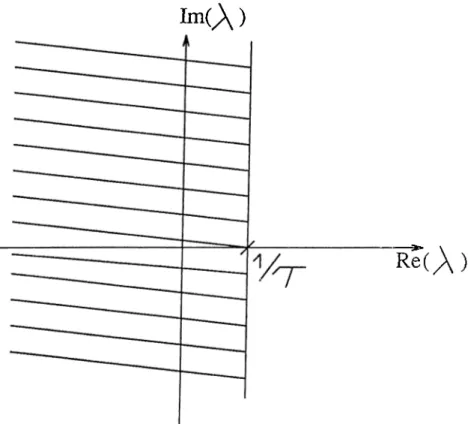
Figure 4.2; Safe region for the eigenvalues of T G
Let G = Then the eigenvalues of ((—l / r ) I + TG ) should be in the left-half of the complex plane. Since the eigenvalues of ((—l / r ) I -f T G ) are the eigenvalues of T G shifted to the left 1/ r , the eigenvalues of T G should be to the left of the line Re{X) = 1/ r , as shown in Fig. 4.2.
Plence, the smaller the r is, the greater degree of freedom one has in choosing the connection weight matrix T without altering asjnnptotic stability.
Using the Theorem 5, it is obtained:
|A „ „(T G )| < <T„„(XG) = lITGII, < IITII2IIGII2 = o„,„,(T)A „„(G ) (4.42) If one chooses
^max (T)A max ( G ) < 1 'max..(T) <
1
(4,43) T Xniaxi^^G^
then the asymptotic stability of the equilibrium Ue is guarcinteed. In .fact, with this choice, the eigenvalues of T G will be confined in the disc whose center is at the origin and whose radius is 1/ r .
CHAPTER 4. ASSOCIATIVE MEMORY DESIGN FOR A CLASS OF NEURAL NETS32 G,· = dg/du\^^j^., z = 1 , . . . , M; and
Amaa.-(G) = maxATOox(G,)
(4.44) Then>(T)<
(4.45) ’^Anгαa;(G)Since
T =
[(l/r)A V x D -i U ']U ^, < \\[(l/r)AV,D-^ ^']h\\C^\\2. is unitary, thus ||U^||2 = 1· Alsocrma.iT) < ||[iA V iD -i U ']||2 < \\^A)ViT>-^\\2 + \\V% (4.46) As a result, if one can choose U' as
l|U'||2 <
-AViD "M
(4.47)‘^Af7joj.(G) T
the memory vectors are guaranteed to be asymptotically stable. For the exis tence of U', the right side of the above inequality should be non-negative which needs further investigation.
Remark 2: Decreasing Xmax(G) will increase the degree of freedom one has in choosing r w’ithout endangering asymptotic stability. To decrease A„,a3,(G), one should choose the equilibrium points on the sigmoid where the slope is small, i.e. close to the asymptotes 1 and -1 (provided a U' exists for (4.47)).
As before, note that the condition given above is only a sufficient condi tion which guarantees the asymptotic stabilit}^. One interesting thing about the conditions for stability is that thej^ are almost the same for continuous and discrete-time models. The bound on the norm of connection matrix
T
is inversely proportional to the maximum eigenvalue of the Jacobian of the nonlinearity (evaluated at the equilibrium points) for both ol the models.Example: Let ^ = 1 in (4), t = 1 in (4.37) and
Xei = 0.9
0.95 , Xe2 =
0.95 -0 .9 so
CHAPTER 4. ASSOCIATIVE MEMORY DESIGN FOR A CLASS OF NEURAL NETSSS
c n y -
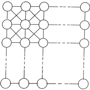
-Figure 4.3: Topology of a cellular neural network
A = 0.9 0.95 0.95 -0 .9 i/(A) 0.4219 0.4422 0.4422 -0.4219 T = 2.1411 -0.0076 0.0076 2.1411 Eigenvalues of T G i and T G 2 come out to be 0.8617, 0.8795 which are to the left of the line Re[X) = 1/ r = 1. Hence, the above condition is satisfied. With initial condition Xqi = (0.925 0.925)^ for Xej and X02 = (0.9
simulations have showed convergence.
0.95)^ for x „ .
4,5
C ellular N eu ral N etw orks
In cellular neural networks [20], each unit is called a. cell and the structure is similar to that found in cellular automata (see Fig. 4.3). Aziy cell in the network is connected only to its neighbor cells and they can intei'cict direct 1\· with each other. Cells which are not neighbors can affect each other indirectly because of the propagation effects of the network. To make neighborhood clear, r-neighborhood of a cell C(i,j), in a cellular neural network is defined Izy ■^^r(bi) = {C(/:, 1) I m ax\k — f|, ]/ — ij < r, 1 < A: < M, 1 < / < A'} where r is a positive integer number.
Our concern with celluhir neural networks is fixed-point programming [21], as in the case of Hopfield model. The design tcisk in this case is finding the connection weights for a certain neighborhood-so that a given set of binar}· patterns U i, U 2, · ■ ·, U^- are fixed points of the net.
CHAPTER 4. ASSOCIATIVE MEMORY DESIGN FOR A CLASS OF NEURAL NETS34
We use discrete time-model with synchronous update rule. At time t, each cell takes feedback from its neighbor cells and total feedback is passed from a signum function, the output of the function becoming the output of that cell. The feedback coming from a neighbor cell is simply the multiplication of the weight connecting the two cells by the output of that neighbor cell at time (i — 1). Here, the case r = 1 is considered.
For cellular neural network structures, ¡patterns are in the form of M x N matrices (see Fig. 4.3). To be able to do the same analysis as we have done in the liopfield case, we bring M x N matrices into vectors of M N x 1 as below:
Uv = U ' = [u,-iUi2 . . . U,w] Ui2
J
(4.48) (4.49)Now the problem resembles to that of Hopfield but because of the. restriction of communicating with only neighbors, T has the specig,! form given below:
T =
Tn T12
0 0 0T21 T22 T23
0 0 0T32 T33 T34
0 0 0 T(A/-l)(A<i-2) T(A/_i)(A/_i) 0 (4.50)where each nonzero block above is in the form of:
CHAPTER 4. ASSOCIATIVE MEMORY DESIGN FOR A CLASS OF NEURAL NETSS5
\
T-· —Bi
C l 0 0 0 A2B
2 C2 0 0 0Bs
C3 0 0 0 Am- 1B
m
.
0 0A
m
(451)(T,j is one of the nonzero blocks given in Eq. (4.50)). An example is provided here to illustrate a specific choice of T. The parameters of each nonzero block T ij are chosen as:
If M is even B\ = B2 = ... = Bm = Cl = C-3 = ... = Cm-1 = A2 — A4 = ... = Am and C 2
=
C 4= . . . —
C m - 2— A3 — A5 — ... —
A m - 1 =0
If M is odd B\ = B2 = ... =■ Bm- 1 = Cl = C3 = ... — Cm-2 = A2 = A4 = . . . = Am- 1 andC, = C4 = ... =
C m ± i= A3 = A
s
= ... =
A m=
B m= 0
U' = / u „ ^ U,-2 (4.52) \ UiA-J
For each vector U( above, partition each subblock into smaller blocks each one containing 2 elements as below (if M is odd, there will be a block containing only one element at the bottom).
CHAPTER 4. ASSOCIATIVE MEMORY DESIGN FOR A CLASS OF NEURAL NETSZ6 = * \ * * (4.53)
V * /
Choose these 2 elements opposite in sign, i.e., 1 and -1. Though this seems to be posing a condition on memory vectors that are to be stored, this is not very serious because there are vectors which satisf}'^ the above condition( [.] denoting the greatest integer function).
C h a p te r 5
C o n c lu sio n
For the CAM design problem, we have presented a characterization of connec tion weights for the continuous and discrete Hopfield neural networks, using hyperbolic tangent and signum functions at the neuron outputs.Similar anal ysis can be used if any other (invertible) nonlinearitj'^ is used at the neuron outputs. Our analysis showed that the choice of connection weights depends on an arbitrary matrix when hyperbolic tangent type nonlinearity is used at the neuron outputs (see (4.11) and (4.40)), and depends on two arbitrary matrices when the signum function is used (see (4.25)). The choice of these matrices affects the performance of the neural network. For that purpose, we presented some sufficient conditions (see Corollaries 1, 2 and Equations (4.17), (4.45)) which guarantee the asjmiptotic stability of the ecpiilibria of the neural network. These conditions pose an upper bound on the norm of the connection weight matrix. For cellular neural networks because of neighborhood constraint, the weight matrix has a special form (see (4.50)) and it brings a restriction on the patterns to be stored.
The choice of the arbitrary matrices mentioned above will affect the stability of the neural network. An interesting problem would be the selection of these matrices so that all the stored memory vectors become asymptotically stable equilibria of the neural network. Another research problem is to incorporate the design methodology presented here with a learning algorithm.