ENVIRONMENTS
a thesis
submitted to the department of computer engineering
and the institute of engineering and science
of b
˙Ilkent university
in partial fulfillment of the requirements
for the degree of
master of science
By
Duygu Ceylan
August, 2009
Asst. Prof. Dr. Tolga K. C¸ apın (Supervisor)
I certify that I have read this thesis and that in my opinion it is fully adequate, in scope and in quality, as a thesis for the degree of Master of Science.
Prof. Dr. B¨ulent ¨Ozg¨u¸c
I certify that I have read this thesis and that in my opinion it is fully adequate, in scope and in quality, as a thesis for the degree of Master of Science.
Assoc. Prof. Dr. Veysi ˙I¸sler
Approved for the Institute of Engineering and Science:
Prof. Dr. Mehmet Baray
Director of the Institute Engineering and Science
MULTI-TOUCH ENVIRONMENTS
Duygu CeylanM.S. in Computer Engineering Supervisor: Asst. Prof. Dr. Tolga K. C¸ apın
August, 2009
Fast developments in computer technology have given rise to different applica-tion areas such as multimedia, computer games, and Virtual Reality. All these application areas are based on animation of 3D models of real world objects. For this purpose, many tools have been developed to enable computer modeling and animation. Yet, most of these tools require a certain amount of experience about geometric modeling and animation principles, which creates a handicap for inex-perienced users. This thesis introduces a solution to this problem by presenting a mesh animation system targeted specially for novice users. The main approach is based on one of the fundamental model representation concepts, Laplacian framework, which is successfully used in model editing applications. The solu-tion presented perceives a model as a combinasolu-tion of smaller salient parts and uses the Laplacian framework to allow these parts to be manipulated simultaneously to produce a sense of movement. The interaction techniques developed enable users to carry manipulation and global transformation actions at the same time to create more pleasing results. Furthermore, the approach utilizes the multi-touch screen technology and direct manipulation principles to increase the usability of the system. The methods described are experimented by creating simple anima-tions with several 3D models; which demonstrates the advantages of the proposed solution.
Keywords: Laplacian mesh editing, mesh segmentation, volume preserving mesh
editing, mesh animation, direct manipulation, multi-touch interaction.
BOYUTLU MODEL CANLANDIRMASI
Duygu CeylanBilgisayar M¨uhendisli˘gi, Y¨uksek Lisans Tez Y¨oneticisi: Yard. Do¸c. Dr. Tolga K. C¸ apın
A˘gustos, 2009
Bilgisayar bilimindeki hızlı geli¸smeler ¸coklu ortam, bilgisayar oyunları, sanal ger¸ceklik gibi ¸ce¸sitli uygulama alanlarının do˘gmasını sa˘glamı¸stır. B¨ut¨un bu uygu-lama alanları 3 boyutlu geometrik modellerin bi¸cimlendirilip canlandırılması pren-sibiyle ¸calı¸smaktadır. Bu nedenle, bilgisayar modellemesini ve canlandırmasını sa˘glayan ¸ce¸sitli ara¸clar geli¸stirilmi¸stir. Fakat, bu ara¸cların ¸co˘gu modelleme ve canlandırma konularıyla ilgili belli bir seviyede deneyim gerektirmektedir. Bu durum, deneyimsiz kullanıcılar a¸cısından bir engel olu¸sturmaktadır. Bu ¸calı¸smada, bu probleme ¸o¨oz¨um olu¸sturmak amacıyla, ¨ozellikle amat¨or kul-lanıcılar i¸cin tasarlanmı¸s bir canlandırma sistemi sunulmaktadır. Benimsenen ana yakla¸sım model bi¸cimlendirme uygulamalarında olduk¸ca ¨onemli kabul edilen Laplace y¨ontemini kullanmaktır. Sunulan ¸c¨oz¨um, bir modelin g¨oze ¸carpan daha k¨u¸c¨uk par¸calardan olu¸stu˘gunu kabul ederek bu par¸caların Laplace y¨ontemiyle aynı anda bi¸cimlendirilmesini sa˘glamaktadır. B¨oylece, modele hareket ediyor hissi kazandırılmaktadır. Hem yerel d¨uzenlemeleri hem de modelin toplu hareke-tini sa˘glayacak etkile¸sim teknikleri geli¸stirilerek daha memnun edici sonu¸clar elde edilmektedir. Son olarak, belirtilen yakla¸sım, ¸coklu dokunmatik ekran teknolo-jisini ve direkt manipulasyon tekniklerini kullanarak sistemin kullanılabilirli˘gini arttırmayı ama¸clamaktadır. Belirtilen metodlar, ¨onerilen ¸c¨oz¨um¨un faydalarını g¨ostermek amacıyla farklı modeller i¸cin basit canladırmalar yaratılarak test edilmi¸stir.
Anahtar s¨ozc¨ukler : Laplace model bi¸cimlendirmesi, hacim korumalı model bi¸cimlendirmesi, model animasyonu, direkt manip¨ulasyon, ¸coklu dokunmatik etkile¸sim.
First and foremost, I would like to thank my advisor Asst. Prof. Dr. Tolga K. C¸ apın for his endless support during my whole Master’s education. He did not only guided me to choose an interesting research topic, but also provided me with all the equipment I needed to accomplish this work. Besides helping me to overcome the problems I encountered in my work, he always encouraged me at the times I felt desperate. Finally, his valuable advice about academic life and assistance in graduate study applications helped me to acquire a chance of pursuing my academic studies in Switzerland.
Many thanks to my other thesis committee members, Prof. Dr. B¨ulent ¨Ozg¨u¸c and Assoc. Prof. Dr. Veysi ˙I¸sler for reading and reviewing this thesis. They also gave me the opportunity to study different applications of Computer Graphics in the courses they had taught and supported my graduate study applications.
I would also like to thank my friend Sezen Erdem for helping me to solve various problems, such as setting up the working environment, fixing certain code debugs, and formatting this thesis. My other friends, Ertay Kaya and Yusuf Saran were mental supporters for me, especially towards the end of my studies. Thanks to Ertay, I did not feel lonely at all during the tough working period and Yusuf always found a way to cheer me up so that I can work with more enthusiasm.
Finally, I am grateful to my parents and my sister, who always believed in me. They always showed respect for my decisions and motivated me throughout my education life.
1 Introduction 1
1.1 Contributions . . . 4
1.2 Organization of the Thesis . . . 5
2 Background 6 2.1 Differential Representations for Editing Operations . . . 6
2.1.1 Overview of Differential Representations . . . 7
2.1.2 Using Discrete Forms in Editing . . . 7
2.1.3 Gradient Field Based Editing . . . 8
2.1.4 Laplacian Surface Editing . . . 9
2.2 Mesh Segmentation . . . 14
2.3 Volume Preserving Shape Deformations . . . 16
2.4 User Interface Design . . . 17
2.4.1 3D Interaction Design . . . 17
2.4.2 Multi-touch Environments . . . 19
3 Approach 20 3.1 Overview of the System . . . 20
3.2 Mesh Processing Component . . . 22
3.2.1 Model Loading . . . 22 3.2.2 Mesh Partitioning . . . 23 3.3 Animation Component . . . 30 3.3.1 Laplacian Framework . . . 32 3.3.2 Volume Preservation . . . 42 3.4 User Interface . . . 46 3.4.1 Multi-touch Environment . . . 47 3.4.2 Interaction Techniques . . . 48
3.4.3 Direct Manipulation Principle . . . 53
4 Results and Discussion 55 4.1 Mesh Partitioning . . . 55
4.2 Laplacian Framework . . . 59
4.3 Volume Preservation . . . 61
4.4 Usability Evaluation . . . 64
1.1 A jump action can be represented with a series of drawings of the individual states of the action. Displaying these drawings one after
another creates an illusion of movement. [40]. . . 1
2.1 A simple mesh. . . 10
3.1 Components of the system. . . 21
3.2 Flow of processes from the users’ point of view. . . 22
3.3 A sample mesh and its data structure. . . 23
3.4 Mesh data structure. . . 23
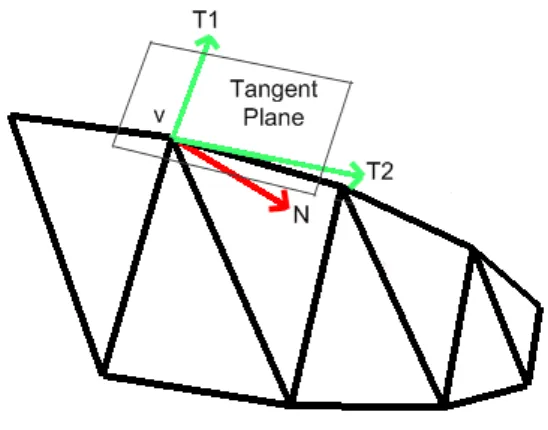
3.5 Principle curvature directions, T1 and T2, of vertex v of a simple mesh is shown. The normal vector of the vertex is denoted by N. . 29
3.6 Mesh partitioning process illustrated for a sample model (a) Nodes obtained after pre-partitioning process, each circle contains the node number and the sign of the average mean curvature. (b) Nodes 0,5,16,10, and 13 are merged to nodes 1,6,9,12, and 15 as a result of Rule-1. (c) Nodes 1,6,9,12, and 15 are merged to nodes 2,7,8,11, and 14 as a result of Rule-1. (d) Nodes obtained after the merging process (e) Model partitioned without merging step (f) Model partitioned with merging step . . . 31
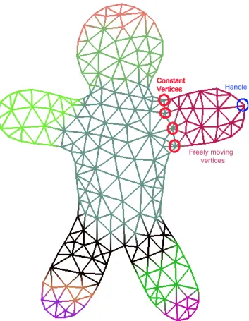
3.7 ROI Specification - Blue vertex is the handle selected by the user. Red vertices constitute the boundary and the in between part is the freely moving part. . . 39
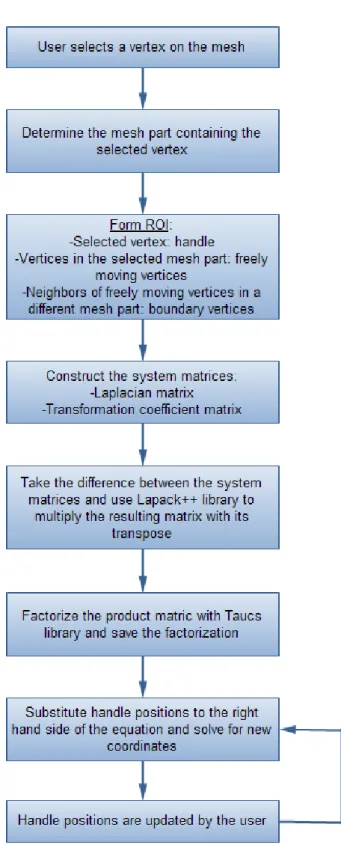
3.8 Flowchart explaining ROI determination and computation of new vertex positions. . . 40
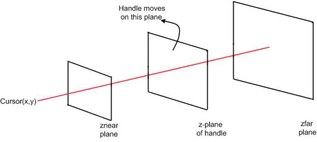
3.9 Cursor positions are projected to the z-plane on which the selected handle lies. . . 41
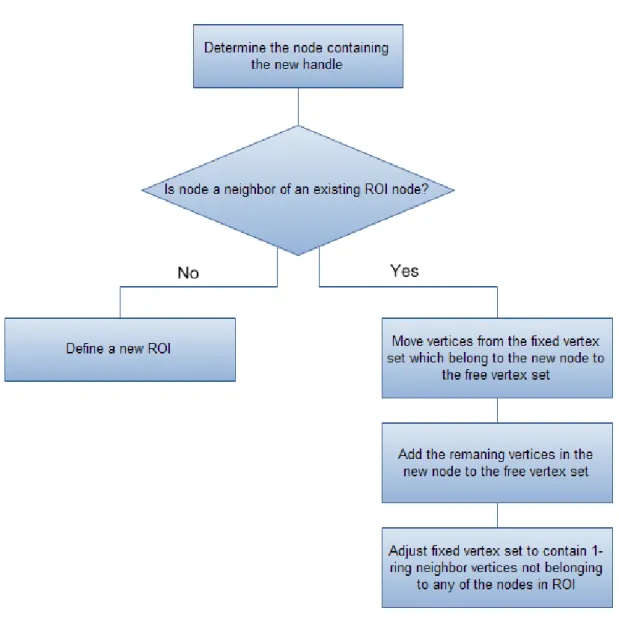
3.10 Flowchart explaining ROI determination with more than one handle. 42
3.11 Vector field is defined from the vertices of a mesh part to the closest points on the bounding box. . . 45
3.12 Laplacian framework uses the result of the previous Laplace oper-ations, whereas the volume preservation component compares the final mesh with the initial mesh. . . 46
3.13 Flowchart of the distinguish operation between single and double clicks. . . 49
3.14 An improved Arcball widget. . . 50
3.15 An example arc between two cursor points, P0 being the cursor
down point and Pi being the cursor up point. . . 51
3.16 Translation vector obtained from cursor points. (a)Cursor moves from the inner region to outer region. (b)First contact with the widget is in the outer region. . . 52
3.17 Non-responsive region in the widget and different translation vec-tors are shown. . . 53
4.1 Mesh partitioning results for a dragon model ((a) and (b)) with different choices of the interval number, k (c) k=5 (d) k=6 (e) k=7 (f) k=8 . . . 57
4.2 Mesh partitioning results for a camel model ((a) and (b)) with different choices of the interval number, k (c) k=6 (d) k=7 (e) k=8 (f) k=9 . . . 58
4.3 A plane model with many details produces a large number of mesh parts. . . 59
4.4 Tail of the fish is manipulated with a single handle shown by the circle. (a) Original model (b) Manipulated model . . . 61
4.5 Arms of the starfish are manipulated with appropriate handles shown by the circles. (a) Original model (b) Manipulated model . 62
4.6 Each wing of the dragon is manipulated with double handles shown by the circles. (a) Original model (b) Manipulated model . . . 62
4.7 Models manipulated by disabling ((a) and (c)) and enabling ((b) and (d)) volume preservation component. Red circles denote the handle positions. . . 63
4.8 User interface of our system . . . 64
4.9 Animation of a dragon model. Transformation widget is visible. . 68
4.10 Animation of a starfish model. Transformation widget is visible in (b), (c), (d), and (e). . . 69
5.1 Prototype design of the extended transformation widget. Orien-tation of the z translation component is adjusted according to the orientation of the index finger shown by an arrow inside the circles. 72
4.1 Partitioning time for different size of meshes . . . 56
4.2 Computation times for matrix multiplication, factorization, and back substitution processes of Laplacian framework, given in seconds. 60
Introduction
Human beings have always had the tendency to make representations of the things they see around them [35]. Man-made drawings found in the caves were the results of this tendency. Yet, single drawings or sculptures were capable of representing only a particular moment in life [35]. Therefore, the search for a means of representing objects or living things in a particular time interval continued. Finally, the invention of motion picture camera and roll film have met this request. By projecting photographs of an action onto a screen, the two instruments have given rise to a new art form. This new art form was called animation [35].
Figure 1.1: A jump action can be represented with a series of drawings of the in-dividual states of the action. Displaying these drawings one after another creates an illusion of movement. [40].
Animation was considered as a very powerful form of art; because it gave the opportunity to represent emotions and thoughts without being limited to a certain set of actions [35]. With the development of color technology, the
effect of animation was increased further. Finally, with the use of computers as modeling and animation tools, the applications of animation art continued to extend, making it a powerful tool for expressing motion, thoughts, and feelings.
Today computer animation is used in many applications, such as computer games, animated web content, and simulators [24]. The variety of these applica-tions give rise to research areas such as realistic object modeling and real-time computer animation. As an illustration, commercial geometric modeling tools have been developed such as 3Ds Max [3] and Blender [8]. These tools focus on creation of 3D objects as well as manipulation of these objects. However, most of these tools require an advanced knowledge or training about the concept, and they are hard to use for inexperienced users. Frequent use of object modeling and animation in computer applications makes the topic of shape modeling and animation an active research area. The deficiency of the commercial animation tools in providing an easy-to-use interface necessitates further research.
Related work to our system can be classified as object creation and object manipulation systems. A number of object creation systems are based on a sketching interface. As an example, Teddy [14] is one of the leading freeform modeling systems, where users are able to model 3D objects within a short amount of time by drawing 2D sketches. Similar easy-to-use object modeling systems have triggered the study of object manipulation. The approaches presented for this purpose fall into a variety of categories. Free form deformation (FFD) is one of the popular categories. In FFD applications, an object is surrounded by a lattice, and editing actions that are applied to the lattice manipulate the object in response. Another important category of modeling solutions is the differential representation. Differential solutions aim to encode shape features of a model and preserve them during manipulation. Obviously, this property of differential approaches makes them popular for realistic and shape preserving editing operations. Because of this, several systems have been developed based on this approach. Some of these system are also sketch-based, in which users define editing commands either by silhouette sketching as in the work of Nealen et al. [23] or gesture sketching as in FiberMesh [22]. There are also systems that involve a direct manipulation interface, where users interact directly with
the object being edited. Examples of this kind include the work of Sorkine et al. [33] and Lipman et al. [19].
The majority of the examples given above focus on building easy-to-use tools for object modeling and local deformations of 3D models. The problem of build-ing animation systems for novice users still exists as an active research area. Traditional methods in computer animation production, such as key-frame ani-mation or motion capture, are not applicable for novice users. These methods either require profound experience about drawing, or complicated and expensive setups. On the other hand, tools designed for inexperienced users should be easy-to-use and should have simple interfaces. In this thesis, we aim to develop a solution for this problem, by building an animation system via enhancing current manipulation techniques. We present a tool which allows intuitive creation of animations.
Our main approach in this work is based on improving differential methods used for model editing operations. We accomplish this improvement by auto-matically defining editing regions on a model and adding a volume preservation mechanism. Both of these improvements have an obvious effect on creating realis-tic animations. We also explore the use of the emerging technology of multi-touch screens. This new technology not only presents a more appealing environment for current desktop interfaces, but also triggers the development of new widgets and gestures. The reasons for using a multi-touch screen in our case are easing animation production and providing a more involving interface. Using multiple fingers instead of only a single mouse cursor enables the object of interest to be edited at several regions simultaneously, thus creating a more realistic anima-tion. Moreover, the multi-touch screen gives the users the feeling of manipulating objects by hand.
1.1
Contributions
In this work we present a novel 3D mesh animation system. We can list our main contributions as follows:
• An automatic scheme for definition of animated model parts. In our system, each 3D model is segmented into semantically meaningful parts, before any editing operation takes place. When the user selects a few ver-tices of the mesh to manipulate, the corresponding parts of the mesh are automatically defined as the animating parts. Therefore, the user does not have to specify which parts of the model are to be affected from the manipu-lation. The segmentation process is based on the fact that humans perceive objects as a collection of smaller parts. As a result, the parts marked as animating coincide with the users’ expectations from the animation of the object of interest.
• Volume preserving mechanism. When physical constraints in 3D an-imation are considered, one of the most important facts that arise is con-servation of mass. When the density of an object remains constant during animation, this implies preservation of volume. For this reason, in our system we combine this physical constraint with our interactive and direct editing framework. Volume preservation is especially important for creating stretch and squash effects that result in a more expressive animation.
• An interface that enables editing operations with direct control. The interface that we are presenting benefits from the growing technology of multi-touch interaction. We combine direct manipulation principles with this technology to give the users direct control over the system. Being able to manipulate models as if holding in hand increases the feeling of immersion.
1.2
Organization of the Thesis
This thesis is organized as follows. Chapter 2 presents related work about the important concepts for our work. These concepts include differential representa-tions for mesh editing operarepresenta-tions, mesh segmentation techniques, 3D user inter-face design, and multi-touch environments. In addition, fundamental notations about these concepts are introduced to enable a better understanding of our work. Chapter 3 describes our approach for designing a mesh animation system targeted for multi-touch environments. This chapter first gives a brief overview of our sys-tem; then details the mesh processing, animation, and user interaction methods that we have applied. Chapter 4 provides the results of our system and discusses both advantages and disadvantages of our work. Finally, Chapter 5 concludes the thesis by summarizing what has been done and what can be considered as a future extension of our work.
Background
In this chapter, we briefly review primary mesh editing techniques based on dif-ferential representations and introduce the fundamentals of Laplacian surface editing. Furthermore, we examine approaches regarding mesh segmentation, vol-ume preserving shape deformations, and user interface design, other dominant notions for our work.
2.1
Differential Representations for Editing
Operations
Meshes are widely used to represent models in computer graphics. A mesh is a collection of vertices, edges, and faces that define the shape of the model being represented. Several different surface representation schemes exist, each exhibit-ing different features of a mesh model. To illustrate, simple triangular representa-tions based on global cartesian coordinates are best for examining the topological structure of the model [31]. However, these simple representations are not ad-equate to carry modeling operations such as mesh editing, coating, resampling etc. Lately, differential representations of surfaces have gained popularity due to their advantages in modeling operations. These representations encode the shape
features of a surface and enable these features to be preserved in a modeling op-eration. In the following sections, we give a more detailed overview of the use of differential representations in one of the most frequent modeling operations, mesh editing. Mesh editing operations are also at the core of our system. We specifi-cally focus on the Laplacian framework, a popular differential representation that we have based our work on.
2.1.1
Overview of Differential Representations
Preserving the shape and geometric details of a model is vital for editing oper-ations. For this purpose, local surface modeling representation approaches have been proposed. Preserving geometric details means minimizing the difference be-tween the deformations of local features of a model. These local features can be encoded via differential representation techniques such as (i) discrete forms, (ii) gradient fields, and (iii) Laplacian coordinates. These encodings are defined by considering each vertex of a mesh with its neighboring vertices. Since differential methods represent local features of a model, minimizing the difference between local features before and after a deformation operation means minimizing the difference between the differential coordinates.
In differential mesh deformation systems, users control the editing process by updating the positions of a few vertices called handles. The new positions of the remaining vertices are derived by considering the handle positions as constraints. The core of this process is to recover global Cartesian coordinates from the de-formed differential coordinates, which requires solving a sparse linear system [33].
2.1.2
Using Discrete Forms in Editing
Discrete form based approaches in mesh editing define a local frame at each vertex, and represent the transition between the adjacent frames in terms of discrete forms. To define a local frame at a vertex, the one-ring neighborhood of the vertex is examined. Each edge connecting the vertex with a neighbor
is projected onto the tangent plane of the mesh at the given vertex. The first discrete form is used to encode the lengths of the projected edges and the angles between the adjacent projected edges, whereas the second discrete form encodes the normal directions. In other words, these two forms represent the geometry of a vertex and its one-ring neighborhood up to a rigid transformation [20]. During manipulation operations, local frames at each vertex are reconstructed from the discrete forms. This problem is expressed as a sparse linear system of equations. Once the local frames are reconstructed, global coordinates are also reestablished by integration of the local frames. This is also expressed as a linear system of equations.
In editing operations, users define a handle vertex to move freely and some boundary vertices which remain fixed to limit the deformation. The positions of these vertices are added to the system of equations to make it over determined. Finally, the over determined system of equations is solved in a least squares manner. The details of the approach are out of scope of this thesis. Readers can refer to the work of Lipman et al. for further information [20].
2.1.3
Gradient Field Based Editing
Gradient field based mesh editing is based on the Poisson equation. The Pois-son equation is an alternative to the least squares problem. To apply PoisPois-son equation to mesh editing, the coordinates of the target mesh are represented as scalar fields on the input mesh. These scalar fields are used to form the gradient field component of the Poisson equation [42]. In editing operations, the gradi-ent fields are transformed by means of transforming triangles. Resulting vector fields are no longer gradients of a scalar function. Therefore, they are considered as guidance vector fields of the Poisson equation and the equation is solved to reconstruct the desired mesh coordinates. Finally, a boundary condition for a mesh is defined by considering the set of connected vertices on the mesh, the set of vertex positions, the set of frames that define local orientations of the vertices, the set of scaling factors, and a strength field. Strength field represents how much a vertex is affected by the boundary conditions and is computed based on
the distance between the initial and final vertex positions. During editing, scale and local frame changes of the constrained vertices in the boundary condition are propagated to the rest of the mesh. For detailed examples of applying this scheme to mesh editing operations, the work of Yu et al. can be examined [42].
2.1.4
Laplacian Surface Editing
Laplacian coordinates are a form of differential representation used widely in mesh editing. Conversion from Cartesian coordinates to Laplacian coordinates requires only a linear operation, whereas the reconstruction of Cartesian coordinates is accomplished by solving a linear system. This linearity of the approach makes it very efficient and it is the main reason why we have also used Laplacian editing in our work. In this section, we look at how these coordinates are defined and used in editing operations.
2.1.4.1 Laplacian Representation
Laplacian coordinates focus on the difference between a vertex and its neigh-borhood. An overview report by Sorkine about the subject describes Laplacian representation in detail [31].
Let global Cartesian coordinates of a vertex i of the connected mesh M be denoted by vi. The Laplacian coordinate (δ-coordinate) of this vertex is defined
as the difference between vi and the average of its neighbors [33]:
δi = vi− 1 di X j∈N (i) vj (2.1)
where N(i) is the set of neighbors of vertex i, and diis the number of neighbors.
Here the δ-coordinate is defined with uniform weights. As stated in the work of Sorkine, uniform weights work sufficiently well in most editing scenarios [33]. However, cotangent weights can be used as well, especially when the considered
mesh is not sufficiently regular [32].
The operation of transforming Cartesian coordinates to δ-coordinates can also be represented with matrices. Let A be the adjacency matrix of the mesh where
Aij is 1 if (i, j) represents an edge, 0 otherwise. Similarly, let D be the
diago-nal matrix such that Dii = di. Then, the Laplacian matrix, L, which converts
cartesian Coordinates to δ-coordinates, is defined as follows:
L = I − D−1A (2.2)
Usually, the symmetric of the Laplacian matrix is used in computations. This matrix can be called as Ls:
Ls= D − A (2.3)
Ls should be normalized before being used to define the transformation of
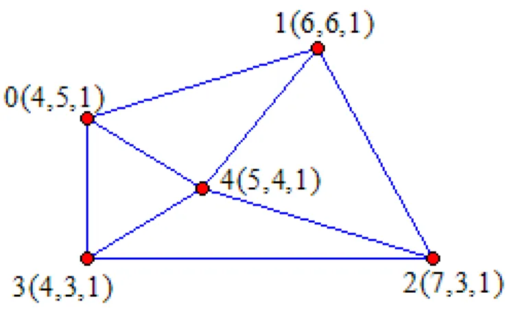
coordinates. We can illustrate this process with a simple example. Assume that we have the simple mesh given in Figure 2.1.
Figure 2.1: A simple mesh.
Ls = 3 −1 0 −1 −1 −1 3 −1 0 −1 0 −1 3 −1 −1 −1 0 −1 3 −1 −1 −1 −1 −1 4
This matrix can be formed by just examining each vertex and its neighbors. For example, the first row of this matrix corresponds to v0 and is computed as
follows. Since v0 has 3 neighboring vertices, the diagonal element becomes 3.
Then, the column elements corresponding to the neighbors of v0 are assigned the
value −1. Rest of the column elements are given the value 0.
Once this matrix is computed, it is normalized by setting the diagonal elements in each row to 1. Then it is substituted into the transformation equation as shown below. (This example uses x coordinates, transformations of y and z coordinates are similar.): Ls∗ v = δ 1 −0.33 0 −0.33 −0.33 −0.33 1 −0.33 0 −0.33 0 −0.33 1 −0.33 −0.33 −0.33 0 −0.33 1 −0.33 −0.25 −0.25 −0.25 −0.25 1 ∗ 4.0 6.0 7.0 4.0 5.0 = −1.0 0.666 2.0 −1.333 −0.25
In conclusion, constructing δ-coordinates from Cartesian coordinates is a straightforward process which requires only a linear operation.
2.1.4.2 Laplacian Editing
The basic idea behind using Laplacian coordinates in mesh editing operations is to perform manipulations on the mesh represented by these coordinates and
reconstruct the global Cartesian coordinates afterwards.
As explained in the previous section, definition of Laplacian coordinates of a mesh is not difficult. However, reconstructing cartesian coordinates from δ-coordinates is more complicated. The immediate reaction to take is to invert the
Ls matrix defined previously. However, this matrix is singular. The singularity
can be shown as follows. The sum of the elements in each row sum up to zero and since this matrix is symmetric, sum of the elements in each column is also zero. In other words, when row vectors of the matrix are added, a zero vector is obtained. Therefore, the last row of the matrix is in fact the sum of the other rows negated. This means, the last row is dependent on the other rows and the matrix rank is less than the matrix size. Since a matrix of size n x n and rank of
r, r < n is singular, the expression x = L−1
s δ is not defined. Therefore, Cartesian
coordinates can be recovered by defining at least one vertex as a constraint and then solving the linear system. We can define this set of vertices as C. These constraints are added to the previously defined system of equations. To illustrate, we assume v0 is a constraint vertex for our mesh and compute the new Lsmatrix:
e L = 1 −0.33 0 −0.33 −0.33 −0.33 1 −0.33 0 −0.33 0 −0.33 1 −0.33 −0.33 −0.33 0 −0.33 1 −0.33 −0.25 −0.25 −0.25 −0.25 1 1 0 0 0 0
This new matrix is named as eL. Each constraint added to the system may
have a different weight, wi. In our example we have used the weight of 1.0.
Adding constraints to the system makes it over-determined, which means it may not have an exact solution. However, the system can be solved in a least-squares sense. Therefore, an error metric is defined for this purpose:
E(v0) = n X i=1 kδi− L(v0i)k 2 −X i∈C wikvi0− cik2 (2.4)
The solution to this least squares problem can be expressed as matrix opera-tions. eL is an (n + m) x n matrix, where n is the number of the vertices in the
mesh, and m is the number of constrained vertices.
v0 = (eLTL)e −1LeTb
(eLTL)ve 0 = eLTb (2.5)
In the above equation, b denotes the right-hand side of the linear system. It is a (n + m) x 1 vector where the first n elements are the δ-coordinates of the mesh vertices, and the remaining m elements are the Cartesian coordinates of the constrained vertices. If we return back to our example, the above equation becomes: (eLTL)ve 0 = eLT ³ −1.0 0.666 2.0 −1.333 −0.25 4.0 ´T 2.2847 −0.6042 0.2847 −0.6042 −0.3611 −0.6042 1.2847 −0.6042 0.2847 −0.3611 0.2847 −0.6042 1.2847 −0.6042 −0.3611 −0.6042 0.2847 −0.6042 1.2847 −0.3611 −0.3611 −0.3611 −0.3611 −0.3611 1.4444 v0 = 3.2847 0.3959 2.2847 −1.6041 −0.3611
The product of a matrix and its transpose is a positive, semi-definite matrix and can be factorized via Cholesky factorization. Therefore, the product (eLTL)e
can also be written as the product of an upper triangular matrix and its transpose,
M = (eLTL) = ( ee RTR). This factorization is used to solve the above equation.e
Remember that an appropriate linear system should be formed for each x,y, and z coordinate to obtain the full solution.
(eLTL)ve 0 = eLTb Mv0 = eLTb ( eRTR)ve 0 = eLTb e Rv0 = x e RTx = eLTb (2.6)
In editing operations, users choose some vertices on the mesh as handles and manipulate them to achieve desired deformations. The manipulations of the handles are propagated to the rest of the mesh until a boundary region is reached. In other words, there is also a set of boundary vertices which remain fixed during manipulation. In order to correctly reconstruct Cartesian coordinates, both the handles and the boundary vertices are defined as constraints to form the above over-determined system. The system matrix is factorized once at the beginning of the editing session and the above equation is solved repeatedly as the movement of the handle vertices change the right hand side vector.
2.2
Mesh Segmentation
As discussed in the previous section, developing different representation schemes of mesh models has been an ongoing research area. Just like differential repre-sentations are useful for encoding shape features, examining a model as a combi-nation of simpler components is an attitude close to human perception [1]. This is the main reason why we have developed the approach of applying mesh editing operations to smaller parts of a model.
Mesh segmentation approaches can be analyzed in two main groups. The first group of approaches concentrate on partitioning a mesh based on some sort of geometric property such as curvature, whereas the second group of algorithms focus on the features of the model to obtain meaningful parts [2].
Among the approaches proposed for the second group of mesh segmentation, the work of Katz. et al. can be listed [17]. This approach follows a two-step algo-rithm. The first step decomposes the mesh into meaningful components keeping the boundaries fuzzy via a clustering algorithm. The second step finds the exact boundaries in accordance with the features of the model such as curvature and the angle between the normals of the adjacent faces of the mesh. Another solution presented by Katz et al. examines all models in a pose-insensitive representation using Multi-Dimensional Scaling (MDS) [16]. Feature points of the model used in segmentation are extracted in this representation. Another approach is Antini et al.’s work, which is based on the visual saliency of the mesh parts [1]. The first step of this algorithm is to compute, for each vertex, the sum of the geodesic dis-tances between the given vertex and the remaining vertices. The sums computed are normalized to a certain range and divided into a constant number of levels, called nodes. The authors comment on the choice of this constant according to experimental results. The second step of the algorithm examines the nodes with respect to adjacency, curvature, and boundary information, and merges some of the nodes with similar properties. To state briefly, the merging step aims to com-bine adjacent nodes with the same sign of average curvature. Each node obtained in the final stage represents a meaningful part of the mesh.
As stated before, in our work, we are interested in applying mesh editing operations into smaller parts of a model. Since the human visual system perceives a model as a combination of visual features, the smaller parts used in our system should be the meaningful parts of the model. Therefore, the second group of mesh segmentation solutions is more suitable for our system. Among the existing solutions given above, our system is based on the approach presented by Antini et al. [1] because it is based on visual saliency. The details of this approach and how we have made use of it are given in the following chapter.
2.3
Volume Preserving Shape Deformations
Animation of an object can be considered as a sequence of manipulation actions applied to it, such as bending, stretching, and compressing. To obtain plausible results, physical constraints should be taken into account during these manipu-lations. Preservation of volume is one of these important animation constraints, which follows from the conservation of mass principle. If the density of an object remains constant during animation, volume is also preserved. For this reason, applications that preserve volume are more advantageous in creating realistic animations.Zhou et al. [43] present a 3D mesh deformation system, which focus on pre-serving volume during large deformations. Their solution is based on building a volumetric graph from a 3D mesh, which contains both the original mesh vertices and the points of a lattice constructed inside the mesh [43]. Volumetric features are represented by the Laplacian coordinates of the nodes of this graph. Volume is preserved by defining an energy function and minimizing it. Work of Hirota et al. [12] is another example system which tries to preserve volume during free form deformations. This approach also defines an energy function similar to potential energy functions for elastic solids and tries to minimize it. This energy function is defined so as to measure deformation and volume preservation constrains the minimization process [12].
In contrast to the examples mentioned above, Funck et al. [38] present a more straightforward mechanism to preserve volume. Even though, this work focuses on mesh skinning applications, authors claim that the volume of a model in an arbitrary deformation can be preserved similarly. This solution first defines a displacement vector field and applies a volume correction step after each defor-mation. The correction step adds the displacement field to the deformed mesh coordinates with appropriate scaling factors in order to preserve the volume be-fore and after deformation.
We base the volume preservation component of our work on the approach presented by Funck et al. [38] because this approach does not require additional
volumetric structures or control components. Therefore, it can easily be adapted to triangular meshes. It is also sufficient to add a volume correction step after Laplacian editing computations so that the overall complexity of the system is not increased.
2.4
User Interface Design
Many graphics applications involve 3D scenes and require users to interact with the scene. Most of these applications work on desktop environments with tradi-tional input devices such as a 2D mouse, whereas some work with devices with more degrees of freedom (DOF). Cubic Mouse [9], ShapeTape [10], and Control Action Table [11] are some of the interesting examples of high DOF devices. Another input device that is gaining high popularity is the multi-touch screen. Different interaction techniques have been developed for these different input in-struments. In this section we review two important examples of these techniques, namely widget-based methods and direct manipulation based techniques. We also discuss recent work on multi-touch environments, which is of our interest in this work.
2.4.1
3D Interaction Design
Interaction design for a 3D application is more challenging compared to the 2D case, because manipulating 3D objects on a computer is a less familiar experience for novice users [13]. Moreover, most of the commonly used input devices supply only 2D information. Therefore, techniques to map 2D input to 3D manipulation tasks should be developed. Another user need related to 3D interaction is that the interaction with the scene should be intuitive. The direct manipulation mode of interaction best suits this second need, because it allows users to directly select objects and apply actions on them. Meanwhile, the display immediately shows the results of the user actions. This is especially important in model design and editing systems. In conclusion, the challenges in 3D graphics applications have
given rise to the design of more effective user interfaces which adopt direct ma-nipulation approach, and the use of gestures and widgets to enhance interaction with the objects in the scene.
Common 3D manipulation tasks include rotation, translation, and scale. Per-forming these operations simultaneously is a challenging task with only a 2D input device, since these operations have more than 2 DOF. Forcing the user to constantly switch between different operation modes makes the interface dis-tracting. The importance of gestures and widgets arises at this point because they are a powerful tool for mapping the 2D input to 3D. Therefore, they are fre-quently used in different applications. As an illustration, the work presented by Draper et al. shows how gestures can be used in Free Form Deformation (FFD), a common model editing scheme [7] . In traditional FFD interfaces, users have to manipulate control points on the lattice of the object, which is a challenging task because it is hard to foresee the result. To overcome this difficulty, Draper et al. [7] present gestures for common operations such as bending, twisting, stretch, and squash. Commands are given by drawing strokes directly on the model itself instead of interacting with the lattice. Similarly, the work of Nealen et al. intro-duces sketch-based gestures for mesh editing via differential representation [23]. The user sketches a stroke to define the silhouette of the mesh part to be edited and performs the editing action by sketching the new shape of the silhouette. This system also enables direct interaction with the object.
3D widgets are as important as gestures in describing 3D editing tasks. They are used to place controls directly in a 3D scene with the objects. Generally each widget connected to an object is responsible for a small set of manipulation operations [5]. As an illustration, a common widget called Virtual Sphere enables the users to rotate an object about an arbitrary 3D axis [6]. The object is assumed to be surrounded by a virtual sphere ball and the user rotates this ball instead of directly rotating the object. Similarly, the technique presented by Houde et al. surrounds an object with a bounding box in the shape of a rectangular prism and places handles at specific positions of the box to perform transformation operations [13]. For example, rotation handles are placed at the corners of the box where as lifting handle is found on the top face of the box.
In conclusion, in the examples given above, users deal directly with the objects in a scene via either a gesture or a widget. This feature enables them to feel more involved in the actions they are taking; making the interface more easy-to-learn.
2.4.2
Multi-touch Environments
As discussed in the previous section, the ability to manipulate objects directly on a screen is appealing for many users, because they feel more involved in the task. Touch screens, especially multi-touch screens, enhance this ability by en-abling users to touch objects on a screen so that they feel like controlling objects directly. For this purpose, these instruments are increasingly used in graphical applications.
The multi-point input feature of multi-touch environments makes them suit-able for gestural interfaces. Therefore, a variety of related work focuses on build-ing gestures and more efficient interaction styles for these environments. As an illustration, Wu et al. presents different gestures for single finger, multi-finger, single hand, and multi-hand usage especially for tabletop displays [41]. The work of Benko et al. is another example which introduces new widgets and interaction methods to enhance clicking and selection operations [4]. Similarly, Rekimoto presents both a multi-touch sensor architecture and new interaction techniques that are hard to implement with a traditional mouse [27].
The nature of multi-touch environments is also well suited for direct manip-ulation interfaces. One of the best examples to illustrate this is the mesh editing system presented by Igarashi et el. [14], which works both in traditional desk-top environments and multiple-point input device SmartSkin [27]. In this system, users are able to directly manipulate 2D meshes displayed on a multi-touch screen by touching and moving them.
On the whole, we can expect multi-touch environments to provide a good means to improve the previously presented approaches in effective interface design with their primary feature of providing multi-point input.
Approach
In this chapter, we present our approach to the problem of interactive mesh animation. Our aim is to develop not only an editing but a simple 3D mesh animation system. The system is designed for multi-touch environments and targeted especially for novice users. The method we have adopted for mesh editing, the additional work done to enable animation, and the principles we have followed in user interface design are discussed in further detail.
3.1
Overview of the System
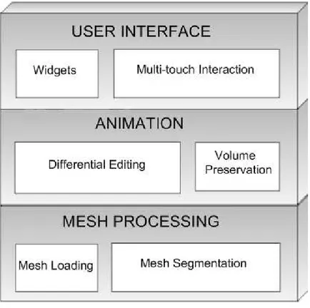
Our mesh animation system is composed of different components: mesh process-ing, animation, and user interface components. To briefly explain, the mesh pro-cessing component loads a model into the system and partitions it into meaningful parts. The animation component is responsible of mesh manipulation operations. Finally, the user interface component includes user interaction techniques. This architecture is summarized in Figure 3.1 and each component is described in detail in further sections.
Our mesh animation system is targeted for a multi-touch screen, but it can work just as well on a traditional desktop computer. The flow of the processes in
Figure 3.1: Components of the system.
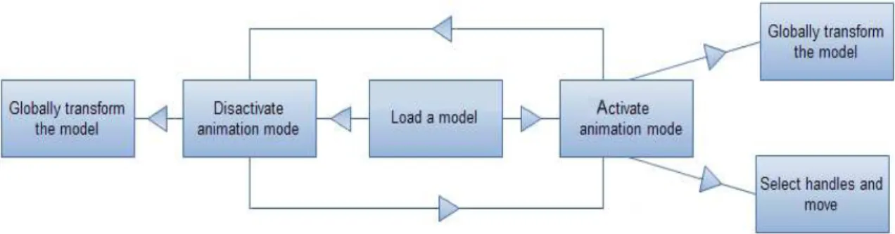
this system from the users’ point of view is as follows. Once a 3D model is loaded to the system, users can start animating it by first switching to the “Animation” mode. Otherwise, the model can only be globally translated, rotated, or scaled. When the “Animation” mode is active, users select a handle by just touching (clicking) the desired location of the model. In the background, the part of the model that will be affected from the editing operation is calculated automatically. The manipulation is based on the “drag-and-drop” principle, which means users move their fingers (or the mouse) which in turn move the handle. Meanwhile, the rest of the affected part is deformed accordingly. By taking advantage of the multi-point feature of the multi-touch screen, users can select as many handles at different locations of the model as they want and deform different parts of the model simultaneously. During the deformation process, the model can also be globally transformed. Users select this command by double touching (clicking) the model which enables a transformation widget. With this widget, users can translate or rotate a model while deforming certain parts of it. This scenario is summarized in the flow chart given in Figure 3.2.
Figure 3.2: Flow of processes from the users’ point of view.
3.2
Mesh Processing Component
In this section, we focus on mesh processing component of our system, which forms the base of the architecture. This component includes two smaller parts, which are responsible for model loading and mesh partitioning. These two parts are described in the coming sections.
3.2.1
Model Loading
The first action to take in order to use our system is to load a 3D model. 3D models loaded should be triangular meshes since further processing operates on triangles. The system currently supports 3D file formats, in which the coordinates of vertices and indices of the vertices forming a face are included. In addition, if the model includes textures, or special material and lighting effects, related information is also read from the model file.
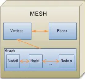
When a model is loaded, the system forms a mesh data structure. The main components of this data structure are vertices and faces. The neighboring rela-tions between these sets are also stored. For each vertex, lists of neighbor vertices and neighbor faces are defined. A face is considered as a neighbor to a vertex, if it contains that vertex. Similarly, for each face, lists of vertices forming the face and neighbor faces are defined. A sample mesh and the corresponding data structure is given in Figure 3.3.
Figure 3.3: A sample mesh and its data structure.
The mesh data structure also contains a graph of nodes that represent the partitioned parts of the model. This graph is completed as a result of the parti-tioning process. Each node mainly contains the vertex indices that are found in the part of the mesh represented by the node. Details of the mesh partitioning process are discussed in the next section.
Figure 3.4: Mesh data structure.
3.2.2
Mesh Partitioning
One of our goals in this work is to extend current mesh editing approaches to enable simple animations. Our main observation is that users tend to animate salient parts of a model. This can be the tail of a fish, the ear of a dog, or the arm of a character. This is due to the fact that the human visual system perceives a
model as a combination of smaller parts. Therefore, a model partitioning scheme should be close to human perception. Based on this observation, in our system, a 3D model is partitioned into meaningful parts. The approach we follow is the method described by Antini et al. [1], which is based on the visual saliency of the parts of a model. This approach can be summarized in two steps. The first step identifies different regions of vertices on a mesh based on distances between them. The second step analyzes these regions and merges some regions according to their adjacency and curvature features. The details of the algorithm are discussed below.
3.2.2.1 Mesh Pre-partitioning
The mesh partitioning algorithm first defines a function on a mesh M with vertices
v based on geodesic distance:
g(vi) =
X
vj∈M
ψ(vi, vj) (3.1)
The above function computes a geodesic distance value for each vertex by summing the geodesic distances between the given vertex and any other vertex denoted by ψ(vi, vj). Dijkstra’s shortest path algorithm is used to compute the
geodesic distance between two vertices [39]. On a mesh, this distance represents the minimum length between the vertices connecting them through the edges of the mesh.
After all the g(vi) values are computed, smallest (gmin) and largest (gmax) of
these values are used to normalize all the values to the range [0,1]:
gnormalized(vi) =
g(vi) − gmin
gmax− gmin if gmin 6= gmax
0 otherwise
(3.2)
The normalized values of g(vi) are divided into a certain number of intervals.
[(k − 1)/n, k/n). This number of intervals affects the number of regions obtained as a result of partitioning and can be fixed or determined with a heuristic. Antini et al. [1] discuss that n = 7 is a reasonable choice according to the experimental results. In our system, users can optionally change this number with a slider. The possible values are chosen as 5,6,7,8, and 9.
Once the intervals are determined, adjacent vertices falling into the same interval are grouped. Each group formed this way is called a node. These nodes form a graph, where two nodes are connected if there exists an edge between two vertices, one from each node. The number of node neighbors of each node can be denoted as ei.
3.2.2.2 Mean Curvature Computation
Several properties are defined for each node in the graph. First of all, boundary vertices of each node are determined. These are the vertices that have no neighbor or have a neighbor in another node. Secondly, the average value of the mean curvature is calculated for each node. For this purpose, the mean curvature for each vertex should be computed. The approach described by Taubin [34] is used for this computation, because it is linear in time and includes simple and direct operations. The details of this algorithm are as follows.
The faces of the triangular mesh M defined before can be called f . For each vertex vi of this mesh, the set of neighboring vertices Ni and incident faces Ii are
defined. Further, the number of neighboring vertices and the number of incident faces at vi are denoted by di and bi.
The curvature computation begins with the estimation of the normals for each vertex as the weighted average of the normals of the incident faces. The weights are proportional to the surface area of the faces.
nvi = X fj²Ii |fj|nfj kX fj²Ii |fj|nfjk (3.3)
In the above equation, nvi and nfj denote the normals of vi and fj whereas
|fj| is the surface area of the face.
Next, for each vertex, a 3 x 3 matrix is formed which has nvi as an eigenvector corresponding to the eigenvalue 0. The formulation of this matrix is as follows:
˜
Mvi = X
vj∈Ni
wijκijTijTijT (3.4)
In the above expression, Tij is defined as the projection of the vector vj − vi
onto the tangent plane hnviTi:
Tij = (I − nvin T vi)(vi− vj) k(I − nvin T vi)(vi− vj)k . (3.5)
κij is the directional curvature in the direction of Tij and is computed as:
κij =
2nT
vi(vj− vi)
kvj− vik2
. (3.6)
Finally, the weight wij is chosen proportional to the sum of the areas of the
triangles that are neighbors of both vi and vj. The number of such triangles is 1
if one of the vertices lies on the boundary of the mesh, 2 otherwise. In addition, for each vertex vi sum of these weights is set to 1.
X
vj∈Ni
As mentioned before, nvi is an eigenvector of the constructed matrix corre-sponding to the eigenvalue of 0. Other eigenpairs should be computed to estimate the principle curvature directions. Taubin advises to form a Householder matrix for this purpose [34]:
Qvi = I − 2WviW
T
vi (3.8)
The steps for computing Wvi given in the above expression are not compli-cated. To begin with, a first coordinate vector E1 = (1, 0, 0)T is defined. If
kE1− nvik < kE1+ nvik, Wvi is equal to the difference between the first coordi-nate vector and the normal vector. Otherwise, it is equal to the sum of the two vectors. Wvi = E1− nvi kE1− nvik if kE1− nvik < kE1+ nvik E1+ nvi kE1+ nvik otherwise (3.9)
The first column of the Householder matrix is equal to either positive or negative nvi. The other two columns called ˜T1 and ˜T2 are used to estimate the principal curvature directions. Since nvi is an eigenvector of ˜Mvi with the eigenvalue 0, the following equality can be written:
QT viM˜viQvi = 0 0 0 0 M˜11 vi M˜ 12 vi 0 M˜21 vi M˜ 22 vi (3.10)
When the 0-row and 0-column are discarded from the above matrix, a 2 x 2 matrix remains. This matrix is diagonalized with Given’s rotation to obtain an angle θ [26]. θ = M˜ 22 vi − ˜M 11 vi 2 ˜M12 vi (3.11)
The angle obtained is used together with the second and third columns of the Householder matrix Qvi, ˜T1 and ˜T2, to find the other two eigenvectors of ˜Mvi.
T1 = cos(θ) ˜T1− sin(θ) ˜T2
T2 = sin(θ) ˜T1+ cos(θ) ˜T2 (3.12)
These two eigenvectors are the principle curvature directions, the curvature values are computed from the corresponding eigenvalues, e1 and e2.
e1 = T1TMviT1
e2 = T2TMviT2
κ1 = 3e1− e2
κ2 = 3e2 − e1 (3.13)
Once the principal curvatures are computed, the mean curvature is simply the average.
κmean= (κ1+ κ2)/2.0 (3.14)
Figure 3.5 illustrates this process by demonstrating the normal vector and the principle curvature directions at a vertex of a simple mesh. The tangent plane,
hNvi
Ti is also shown.
3.2.2.3 Merging of Nodes
After the mean curvature for each vertex is computed as described, the average mean curvature for each node is easily calculated. This property together with the boundary properties is used to join adjacent nodes because the mesh could be over-segmented at this stage. In other words, after all of the nodes and their
Figure 3.5: Principle curvature directions, T1 and T2, of vertex v of a simple mesh is shown. The normal vector of the vertex is denoted by N.
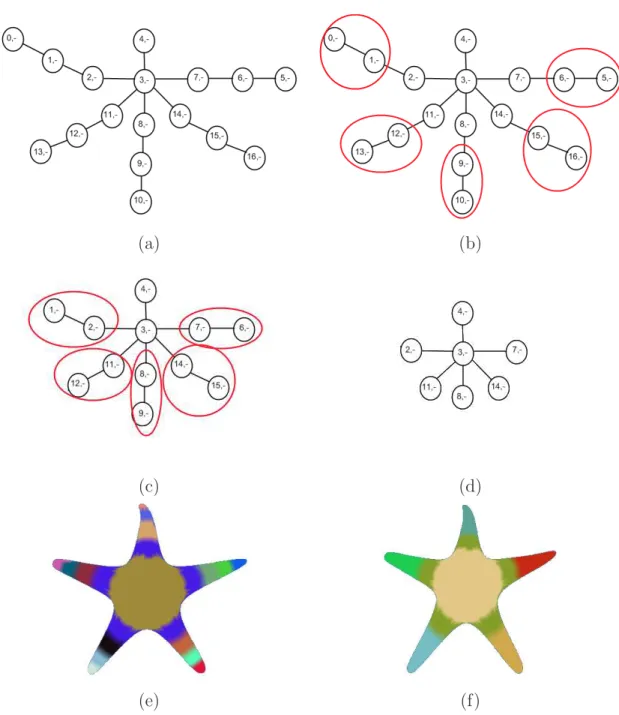
properties are defined, the second stage of the segmentation algorithm begins, in which some nodes are merged together. Anitini et al. [1] have defined some rules to carry out this process. These rules that should be applied in order are listed below.
• As long as there is a node, i, with only one neighbor, that single neighbor, called node j, should be examined. If the number of neighbors of node j is less than or equal to 2 and the sign of the average mean curvature of both node i and node j are the same, the two nodes are merged.
• As long as there is a node, i, with two neighbors, both of the neighbors should be examined. If for a neighbor, called node j, the number of neigh-bors is less than or equal to 2 and the sign of the average mean curvature of both node i and node j are the same, the two nodes are merged.
• As long as there is a node, i, with more than or equal to two neighbors, each of the neighbors are examined. If for a neighbor, called node j, the number of neighbors is greater than or equal to 2 and the sign of the average mean curvature of both node i and node j are the same, the two nodes are merged.
After the second phase of the algorithm is completed, a reasonable amount of mesh parts are obtained. This algorithm is summarized in Figure 3.6. As a final note, the segmentation task explained takes a reasonable amount of time especially when the mesh size grows. For this reason, the partitioning is done as a preprocessing step, and the results are stored as a file in our system so that when the same model is to be segmented with the same choice of interval number, the result can be loaded automatically from the file.
3.3
Animation Component
In this section, we primarily focus on how the meaningful parts of a model ob-tained as described in the previous section are used in animation production. Our main objective in this work is to provide users with the opportunity to cre-ate simple realistic animations by enhancing mesh editing techniques. As stcre-ated previously, users tend to animate salient parts of a model. For this reason, our system allows editing operations to be applied to the meaningful parts of the mod-els. In addition, we provide both an editing and global transformation interface to enable users to translate and rotate a model while deforming. This results in more realistic animations. Finally, the use of a multi-touch screen has an evident effect in animation, since being able to deform different parts of a model simul-taneously creates more expressive results. Even though all the stated features have a positive effect on building an animation tool, the mesh editing technique used has a special importance since it directly affects the results. Therefore, the core of the animation component is the mesh editing process. As discussed in the previous chapter, the method we have adopted for this purpose is based on differential representations that have gained a high popularity lately. The logic behind this choice is to be able to benefit from the advantages of differential meth-ods. These methods are best for encoding shape features of a model and thus suitable for detail-preserving mesh deformations [31]. We particulary focus on Laplacian framework because conversion from absolute Cartesian coordinates to Laplacian coordinates is a straightforward operation, whereas the reconstruction of the Cartesian coordinates can be achieved by solving a sparse linear system
(a) (b)
(c) (d)
(e) (f)
Figure 3.6: Mesh partitioning process illustrated for a sample model (a) Nodes obtained after pre-partitioning process, each circle contains the node number and the sign of the average mean curvature. (b) Nodes 0,5,16,10, and 13 are merged to nodes 1,6,9,12, and 15 as a result of Rule-1. (c) Nodes 1,6,9,12, and 15 are merged to nodes 2,7,8,11, and 14 as a result of Rule-1. (d) Nodes obtained after the merging process (e) Model partitioned without merging step (f) Model partitioned with merging step
[33]. The linearity of this approach makes it appealing for real-time use and the ability to preserve geometric properties in the reconstruction step is a necessity for many modeling operations. On the other hand, Laplacian surface editing does not focus on volume preservation, which is an equally important concept for realistic animations. Thus, our animation component also includes a volume preservation unit. The following sections detail both of these parts and underline the improvements accomplished.
3.3.1
Laplacian Framework
Laplacian framework is best suited for encoding the shape features of a model be-cause each vertex of a mesh is considered within its neighborhood. This property of the framework enables reconstruction of Cartesian coordinates as outlined in Chapter 2, while preserving geometric details of the model. On the other hand, the main practical problem with Laplacian coordinates is their variance to scal-ing and rotation operations. This leads to the fact that reconstructed Cartesian coordinates once a mesh undergoes a linear transformation are erroneous. For this reason, some sort of a scheme should be developed to compensate for this deficiency. Different solutions have been proposed for this problem. In Lipman et al.’s work [19], explicit rotations are estimated by defining a local frame for each vertex. The system is solved again considering these estimations. The pro-cess is repeated until a smooth result is obtained. Yu et al.’s work [42] also uses explicit assignment of rotations, but the rotations of the handles are defined by the user and propagated to the other vertices proportional to geodesic distance. In contrast to explicit methods, Sorkine et al.’s work [33] presents an approach where the transformation of each vertex is computed implicitly. This approach has been applied to 2D mesh editing in the system presented by Igarashi et al. [14].
Yet, not all the example solutions given above are applicable in our case. To illustrate, the rotation estimation method discussed by Lipman et al. [19] requires many iterations to achieve smooth results for complex models [31]. Similarly, the approach of Yu et al. [42] requires users to define explicit rotations which can be
considered as a very challenging task for novices, the target group of our system. Regarding these facts, the solution based on implicit computation of rotations presented by Sorkine et al. [33] is more suitable for our work.
Recall that editing operations are applied to a mesh M with vertices v. The main idea of computing implicit rotations is to define a similarity transformation matrix, Ti, and to represent this matrix as a function of the unknown vertex
co-ordinates. In other words, the least squares formulation to reconstruct Cartesian coordinates provided in the previous chapter becomes:
E(v0) = n X i=1 kTi(v0)δi− L(v0i)k 2 −X i∈C kv0 i− cik2 (3.15)
Although both Ti and v0 are unknown in the above function, when Ti is
rep-resented as a linear combination of v0 there is only one unknown left. The logic
for defining Ti also lies in considering each vertex within its neighborhood. The
corresponding formulation is given in the work of Sorkine et al. [33] as follows:
E(v0) = min Ti (kTivi− v0ik2+ X j∈Ni kTivj − vj0k2) (3.16)
Here each Ti transforms the 1-ring neighborhood of a vertex to its new
loca-tion. Sorkine et al. [33] claim that each transformation should be constrained to allow free rotation and isotropic scaling in order to avoid shearing. True 3D rota-tions cannot be expressed linearly in 3D; a linear approximation can be developed, however. The approximation proposed by Sorkine et al. [33] is as follows:
Ti = si −hi3 hi2 hi3 si −hi1 −hi2 hi1 si (3.17)
As shown with this matrix, finding Ti means finding the unknown coefficients
which can be represented by the vector (si, hi)T. The transformation Tivi can
Pi = vx 0 vz −vy vy −vz 0 vx vz vy −vx 0 (3.18) Tivi = Pi(si, hi)T (3.19)
The minimizer function for Ti given above can be rewritten as
E(v0) = min kA
i(si, hi)T − bik2 (3.20)
where the 3m x 4 matrix Ai (where m is the number of neighbors of vi plus 1)
is formed by writing the P matrices for the corresponding vertex and its neighbors one below the other. Similarly, bi is the vector formed by writing the x,y, and z
coordinates of v0
i and its neighbors. An example of these variables corresponding
to the vertex v0 in Figure 2.1 is given below:
A0 = 4.0 0 1.0 −5.0 5.0 −1.0 0 4.0 1.0 5.0 −4.0 0 6.0 0 1.0 −6.0 6.0 −1.0 0 6.0 1.0 6.0 −6.0 0 4.0 0 1.0 −3.0 3.0 −1.0 0 4.0 1.0 3.0 −4.0 0 5.0 0 1.0 −4.0 4.0 −1.0 0 5.0 1.0 4.0 −5.0 0
(si, hi)T = (ATi Ai)−1ATi bi (3.21)
In the general least squares problem given in Equation 3.15, there is an ex-pression of Ti(v0)δi. Just like defining Tivi as the multiplication Pi(si, hi)T, this
expression can also be redefined. Letting Fi be the matrix
Fi = δx 0 δz −δy δy −δz 0 δx δz δy −δx 0 (3.22)
which contains Laplacian coordinates, δ-coordinates, of vi, Ti(v0)δi can be
rewritten as Fi(si, hi)T. Moreover, the expression for (si, hi)T can be replaced
with the equality given in Equation 3.21. (Since bi contains the positions of vi0
and its neighbors, it is replaced with v0.)
Fi(ATi Ai)−1ATi v0 (3.23)
The expression Fi(ATiAi)−1ATi represents a 3 x 3m matrix, where m is the
number of neighbors of vertex vi plus 1(for itself). The first three columns of
this matrix corresponds to the vertex itself, while rest of the columns correspond to the neighboring vertices. This matrix is multiplied by bi which contains the
positions of v0
i and its neighbors. The positions are placed in the same order of
the columns of the matrix. If the positions of all v0
i are written one below the
other, a 3n x 1 vector is obtained. This vector can be multiplied with a 3n x 3n matrix formed by writing the 3 x 3m matrices one below the other. However, in order to obtain a matrix with 3n columns, for each vertex matrix, the columns corresponding to the vertices that are not a neighbor should be filled with a 0. This process is illustrated for the example mesh given in Figure 2.1. In the example given below, cij represents the 3 x 1 vector corresponding to the columns
F0(AT0A0)−1AT0v0 = ³ cx 00 cy00 cz00 cx01 cy01 cz01 cx03 cy03 cz03 cx04 cy04 czc04 ´ ∗ ³ v0 0x v0y0 v0z0 v1x0 v01y v1z0 v3x0 v03y v3z0 v4x0 v04y v04z ´0 T ⇓ overall equation à cx 00 cy00 cz00 c01x cy01 cz01 0 0 0 cx03 cy03 cz03 cx04 cy04 czc04 ... ! ∗ ³ v0 0x v0y0 v0z0 v1x0 v1y0 v1z0 0 0 0 v3x0 v3y0 v3z0 v4x0 v4y0 v4z0 ´T (3.24)
The 3n x 3n transformation coefficients matrix shown above can be repre-sented as M. After substituting M into the general least squares equation, only one unknown, v0, is left.
E(v0) = n X i=1 kTi(v0)δi− L(v0i)k 2−X i∈C kv0 i− cik2 = n X i=1 kMv0− L(v0)k2−X i∈C kv0 i− cik2 = n X i=1 k(M − L)v0k2−X i∈C kv0 i− cik2 (3.25)
As shown above, in order to compensate for the general linear transformations, the Laplacian matrix found in the least squares problem is replaced with M − L, called A. From this point on, the solution is just like the problem in the case that ignores linear transformations. The difference is that, instead of solving 3 (n x n) matrix systems corresponding to x,y, and z coordinates, a single (3n x 3n) system is solved.