Regional Technical Inefficiencies in Agriculture
Nazmi Demir and Syed F. Mahmud
Assistant and visiting associate professors, Bilkent University, 06533 Bilkent, Ankara ,Turkey
(phone: 90-312-2901640; fax: 90-312-2904383; e-mails: [email protected]; [email protected]).
Received January 2002, accepted August 2002
A survey of applications of the Technical Inefficiency Effects (TIE) model suggests that agro-climatic and other environment variables are customarily omitted in the model specifications. The justification for such an omission is the assumption that these variables are beyond the control of the farmers and therefore should be treated as random variables. In this paper, we argue that in applications dealing with regional agricultural data, agro-climatic variables should not be treated as pure random terms. Historical differences in agro-climatic conditions are known with a reasonable degree of certainty across a larger region. Therefore, omission of such variables from the analysis may lead to inaccurate interregional technical inefficiency comparisons. In order to demonstrate the importance of agro-cli-matic variables in such analyses, we estimate the TIE model for Turkey. A translog stochastic frontier production function with agro-climatic variables such as rainfall and land quality is estimated, and it is shown not only that the agro-climatic variables are statistically significant but also that their omis-sion substantially affects mean output elasticities and relative technical efficiencies.
Une étude sur les applications du modèle de l’effet d’inefficacité technique (EIT) laisse à supposer que les variables agro-climatiques et les autres variables environnementales sont comme d’habitude omis-es dans lomis-es spécifications du modèle. Une telle omission omis-est justifiée par l’hypothèse selon laquelle comis-es variables sont en dehors du contrôle des fermiers et devraient être considérées comme des variables aléatoires. Dans ce communiqué, nous affirmons que dans les applications concernant les données agricoles régionales, ces variables agro-climatiques ne doivent pas être traitées comme de simples ter-mes aléatoires. Les différences historiques dans les conditions agro-climatiques sont connues avec un degré raisonnable de certitudes pour une grande région. Aussi l’omission de telles variables dans l’analyse peut-elle donner lieu à de fausses comparaisons interrégionales d’inefficacité technique. Afin de démontrer l’importance des variables agro-climatiques dans de telles analyses, nous considérons le modèle de l’effet d’inefficacité techniques de la Turquie. Il s’agit d’une fonction de production frontal-ière translogue et stochastique avec des variables agro-climatiques telles que la pluviosité, la qualité de sol et d’autres variables. Nous démontrons que les variables agro-climatiques sont non seulement importantes statistiquement, mais que leur omission influence essentiellement les élasticités moyennes de production ainsi que les efficacités techniques relatives.
Canadian Journal of Agricultural Economics 50 (2002) 269–280
INTRODUCTION
The standard parametric approach to the measurement of technical efficiency (TE) in agricul-ture entails an estimation of a stochastic frontier production function, with a composite error term (Aigner, Lovell and Schmidt 1977; Meeusen and van den Broeck 1977).1The composite
term involves an unobservable random variable related to the technical inefficiency of the farms and a random error in a typical regression model. The latter is assumed to capture random vari-ations in agricultural output due to measurement errors and varivari-ations in other factors that are beyond the control of the farmers. Various distributional forms have been employed for the error term associated to technical inefficiency.2For example agro-climatic conditions such as
land quality and rainfall could be considered as one of the sources of such random variations. Agro-climatic and other environmental variables are normally ignored in the empiri-cal specification of agricultural stochastic production function models, on the assumption that they are beyond the control of the farmers. In this paper, we argue that the differences in agro-climatic conditions are historically known across various agricultural zones and therefore should not be treated as random.3The exclusion of these variables may
incor-rectly attribute the impact, on TE levels, of agro-climatic conditions to the farms and/or agro-regions. Moreover, the uncontrollable agro-climatic factors interact with land, labor and capital inputs and so the use of inputs is likely to depend on factors such as rainfall. If we decide to include agro-climatic conditions, the concept of model specification also becomes an important issue. Different specifications of the technical inefficiency effect (TIE) are proposed in literature (for example, Battese and Coelli 1995; Battese and Broca 1997). In this paper, we attempt to account for the effects of agro-climatic variables on TE with different model specifications using aggregate provincial data. We expect more mean-ingful estimates of TE measures for the provinces by disentangling the possible effects of the location-specific environmental variables. A translog stochastic TIE model is applied to represent data from 67 provinces of Turkish agriculture for the period 1993–95. Model interactions of uncontrollable factors with level of input usage are also incorporated through a nonneutral specification of the TIE. We think that interregional comparisons of TE measures in agricultural production may become more useful for agricultural policy decision making when the uncontrollable environmental effects are incorporated in the analysis.
Review of the studies of agricultural production frontiers employing provincial or regional data suggests that these models primarily focus on farm-specific characteristics while estimating technical efficiencies and show no concern to the broader environmental factors, such as soil quality and climatic conditions.4Ali and Chaudhry (1990) employed
Punjab data in Pakistan, Brada and King (1994) analyzed data on different agricultural regions of Poland, Kalirajan, Obwona and Zhao (1996) worked with data from Chinese provincial-level agriculture, and Battese, Malik and Gill (1996) analyzed data on four dis-tricts of Pakistan. All these studies, which employed provincial and/or regional data, ignored environmental variables in their analysis.5
THE MODEL
We follow Huang and Liu’s (1994) work on the Taiwanese electronic industry. Huang and Liu introduced the assumption of nonneutral effects in their model in which interaction terms between firm-specific factors and production inputs were incorporated. Battese and Broca (1997) also used these interactions to further explain technical inefficiency. This nonneutral model is useful in agricultural applications where one would expect that farm-specific vari-ables such as the education of the farmer would have a different effect on technical ineffi-ciency at different levels of inputs. In this paper, we incorporate this framework using
aggre-gate provincial level agricultural data as opposed to farm level data. We also assume that agro-climatic variables may affect the productivity and therefore we include these variables in the production function as well as in the inefficiency model.
The model specification is:
(1) where:
subscripts i and t = the ith province (i = 1, 2, . . ., 67) and the tth year of observation
j, m = A, L, K, Q, R
VAit= the agricultural value-added in province i
X variables = land, A, labor, L, capital, K, land quality, Q, and precipitation, R.
The Vit’s are assumed to be independent and identically distributed as normal random
variables with zero mean and constant variance σv2, and are also assumed to be independent
of the Uit. The Uit’s are assumed to be nonnegative and independently distributed random
terms, which are obtained by truncation (at zero) of a normal distribution with variance σ2 and mean µit, where µitis defined as:
(2) The Z variables include, land ownership distribution (measured by Gini coefficient G), land quality (measured by a land quality index Q), general cropping pattern (a dummy vari-able taking 1 for intensive cultivation, 0 for cereals and traditional livestock C) and rainfall (a dummy variable taking 1 for precipitation above the national average R), and δ’s are the parameters to be estimated. Maximum likelihood estimates of all the parameters of Eqs. 1 and 2 were obtained simultaneously using the program FRONTIER 4.1 (Coelli 1996). The spe-cific forms of these likelihood functions, which are to be maximized, are reported in Battese and Coelli (1993) and Huang and Liu (1994).
DATA AND DISCUSSION OF RESULTS
Data from 67 provinces, aggregated at provincial level, covering the years 1993, 1994 and 1995 have been employed in this paper. A summary of variables is provided in Table 1.
The value-added from agriculture (crop and animal husbandry) averaged TL206 billion (TL is the Turkish currency unit) in 1987 prices. The standard deviations show there is con-siderable variation among provinces. The size of the standard deviations indicates large interprovincial differences in agricultural land, labor and capital. Capital is a linear combi-nation, based on the principal-component approach, of various agricultural capital stocks including agricultural machinery.6The dummy for general crop pattern is 1 if a province
derives more than 50% of its agricultural output, in value, from intensive cultivation (gen-erally industrial crops, fruits and vegetables). Land quality is the percentage of areas in top quality 4 classes in all agricultural land (8 classes). Land quality in each class is a combina-tion of topography, soil fertility, soil texture and other factors (KHGM). Land ownership distribution is measured by Gini coefficients estimated for provinces from the Agricultural Census data for the year 1991 (DIE 1994) and assumed to be constant for the period 1993–95. lnVAit jlnXjit jmlnXjitlnX V U m j j mit it it =β0+
∑
β +∑
∑
β + − µit δ δj jit δ j jk jit k j kit Z Z X = 0+∑
+∑
∑
4 4 3 lnTable 1. Descriptive statistics for variables in the stochastic frontier model for provinces, Turkish agriculture, 1993–95 Agricultural Agricultural Land Land Sample Value-added land labor Capital index ownership quality index Crop pattern Precipitation (million TL (ha) (person-years) (dummy =1 (dummy =1 if in 1987 prices) for noncereal above national base) average) Mean 206230 347223 342482 100 0.518 0.734 0.239 0.403 Standard deviation 178784 303518 178965 59 0.068 0.201 0.427 0.492 Minimum 15505 59135 66627 7 0.355 0.140 0 0 Maximum 906617 2160370 949851 271 0.714 0.980 1 1
Source: Value-added, agricultural land, agricultural labor data come from the State Institute of Statistics (SIS), National Inc
ome Accounting Tables,
Statistical Yearbook and Agricultural Structure. Rainfall data are from the General Directorate of Meteorology in diskettes. St
atistics on land quality
come from the Village Affairs Organisation (KHGM). Estimates of Gini coefficients are based on the General Agricultural Census
of 1991 in Turkey
The maximum likelihood estimates of the parameters of the translog stochastic frontier production function in Eqs. 1 and 2 together with those of three submodels with various restrictions are given in Table A-1 of the Appendix. One would generally expect het-eroscedastic error structure while using provincial data. With the Goldfeld-Quandt test, we did not find any evidence for the presence of the heteroscedasticity. Model 1 does not include any agro-climatic variables. Model 2 includes agro-climatic variables only in the inefficien-cy function with neutral effects. Model 3 is a nonneutral specification with agro-climatic vari-ables in the TIE function. Three separate null hypotheses were tested using the likelihood ratio test and the results are presented in Table 2.
All the null hypotheses in question were strongly rejected by the data. And therefore no sub-model that is considered is an adequate representation for the data, given the specification of the stochastic frontier model in Eqs. 1 and 2 (see Table 2).7Given Model 4, the null hypothesis that
all coefficients associated with the agro-climatic variables are zero (Model 1) is strongly reject-ed and therefore Model 1 does not adequately represent the data. The second null hypothesis that the neutral specification together with restrictions that rainfall and land quality have no effect on productivity and efficiency, given Model 4, is also rejected. Finally, the rejection of the third null
Table 2. Tests of null hypotheses based on the likelihood ratio statisticafor parameters of the
stochas-tic frontier production function for provinces in Turkish agriculture
Null hypotheses Meaning of the Log-likelihood Critical
null hypotheses function γ values at 5% Decision Model 4
Given the nonneutral –30.7
translog model Model 1
H0:δG= δQ= δC= δR= 0 There are no linear and –87.1 50.6 38.89 Reject H0 and Model 2 restrictions interaction terms for TIEs,
and R and Q have no effect on productivity and efficiency
Model 2
H0: δij= 0 and Neutral model is adequate –61.8 40.2 33.92 Reject H0 Model 3 restrictions and R and Q have no effect
on productivity and efficiency Model 3
H0: βQ= βR= βQQ= βAQ R and Q have no effect on – 41.7 22.0 18.31 Reject H0 = βAR= βLQ= βLR= βKQ productivity
= βKR= βQR= 0
aThe likelihood ratio is γ= –2 Ln (H
0/H1) where H0and H1are the likelihood functions under the null
and alternative hypotheses respectively. d.f. = Number of restricted parameters.
hypothesis, that the two agro-climatic variables rainfall and land quality have no effect on pro-ductivity, implies that even Model 3, with three traditional production inputs together with the environmental variables, does not adequately represent the data. We were particularly interested in the significance of the agro-climatic variables and most of them in both neutral and nonneu-tral models were found to be significant. All the coefficients carry the correct signs (negative) as expected. In the neutral specification (Model 2) except for the Gini coefficient, all other coeffi-cients are significantly different from zero. For the nonneutral model (Model 4), the marginal contribution of environmental variables to the technical efficiency has been computed as indi-cated in Battese and Broca (1997). The terms ∂E(e–u) / ∂Zkare functions of variable inputs, X’s, and therefore these marginal contributions have been evaluated at sample means. The marginal contributions to technical efficiency are estimated to be 0.658 for Gini, 0.073 for land quality, 0.102 for general crop pattern and 0.166 for rainfall. These results indicate that technical effi-ciency is positively related to the environmental variables.
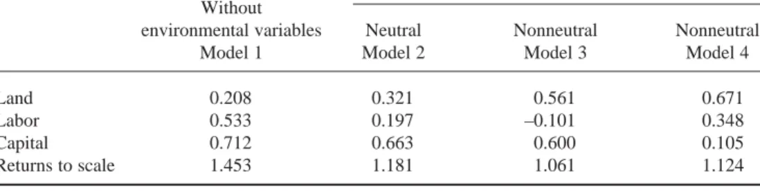
Elasticities of mean output with respect to land, labor and capital for the Model 1 and Model 2 are read directly from columns 2 and 3 of Table A-1 in the Appendix. The input variables employed are mean corrected and therefore the first-order parameters of Model 1 and Model 2 are output elasticities evaluated at sample means. They all are significant, except for the coefficient of land in the neutral model. For the Model 3 and Model 4, the elasticity of mean output [∂Ln E(VAi) / ∂Ln Xk] equals the elasticity of the frontier output (or the elasticity of best practice production) with respect to input k minus the elasticity of technical efficiency with respect to input k [Ci(∂ µi/∂Ln Xk)] where the value of Ciis deter-mined by the density and distribution functions, given µi and σ of the standard normal random variable (Huang and Liu 1994; Battese and Broca 1997). The elasticities and returns to scale estimated at the mean levels of inputs and of environmental variables are presented in Table 3.
The elasticities of mean output with respect to inputs are positive in all models except for the elasticity of output with respect to labor in Model 3.8In Model 4, a 1% increase in
land, labor and capital contributes 0.67, 0.35 and 0.11%, respectively, to the mean output. The largest contribution to the mean output comes from land.
TECHNICAL EFFICIENCIES
The descriptive statistics of the technical efficiency (TE) from the translog stochastic frontier for the four models are reported in Table 4. The inclusion of the environmental variables and specification of the models do appear to affect mean technical efficiency. The result suggests that the average performance, in terms of technical efficiencies, of the provinces based on Model 4 is 62% compared with that of the best practice provinces. The standard deviation of the mean efficiency from Model 4 is found to be considerably larger than the other models. A similar result was obtained by Huang and Liu (1994, 177). One explanation of this result could be that in the nonneutral specification, the marginal contribution of production inputs also depends on the agro-climatic conditions in each province. Thus, provinces with different levels of factor input utilization are expected to gain (or lose), in terms of TEs, directly or through interactions with favorable (or limiting) agro-climatic conditions with the result of a wider range of TEs than those of the neutral one.
These differences in mean technical efficiencies and standard deviations are also high-lighted from the frequency distributions of TE scores in Figures, 1a, 1b, 1c and 1d. The
rank-ing of provinces, in terms of their technical efficiency scores, changes considerably for dif-ferent model specifications and difdif-ferent regions.
As expected, when the agro-climatic conditions are taken into account, provinces at locations with relatively unfavorable environmental conditions, such as the middle and east-ern regions, are able to gain in terms of technical efficiency and vice versa. For example, the TE of Gümüshane, a province in the eastern region with poor land quality and lesser amounts of precipitation in general, increased from 32% (Model 1) to 79% when environmental effects with nonneutral specifications were incorporated (Model 4). In contrast, the TE of Istanbul located on the coastal region generally with favorable agro-climatic conditions, was estimat-ed at 34% when no environmental effects were incorporatestimat-ed and it was down to 16% when environmental effects were assumed with nonneutral specification. The spread of TE scores is considerably increased with Model 4 (Figure 1d). Figures 2a and 2b highlight changes in TE scores from Model 1 and Model 4 in the coastal and noncoastal regions. Furthermore, changes in TE scores are more pronounced in the coastal than noncoastal regions. One may also observe significant changes in the size and spread of TE scores when agro-climatic vari-ables are incorporated in the production and TIE functions. One explanation may be that the agro-climatic conditions in the coastal provinces are more heterogeneous than those in the noncoastal provinces. For example, the standard deviation of land quality index is 0.24 for the coastal and 0.1 in the noncoastal regions.
The estimate of γparameter in all the models is fairly close to one, except in Model 4 where it is 0.763 (see Table A-1).9While the estimate of γparameter for Models 2 and 4 are
significantly different from one, those for Model 1 and 3 are not.
Table 3. Elasticities of mean output and returns to scale with and without environmental variables inputs With environmental variables
Without
environmental variables Neutral Nonneutral Nonneutral
Model 1 Model 2 Model 3 Model 4
Land 0.208 0.321 0.561 0.671
Labor 0.533 0.197 –0.101 0.348
Capital 0.712 0.663 0.600 0.105
Returns to scale 1.453 1.181 1.061 1.124
Table 4. Descriptive statistics of TEs from four models for 67 provinces of Turkish agriculture With environmental variables Without
environmental variables Neutral Nonneutral Nonneutral
Sample Model 1 Model 2 Model 3 Model 4
Mean 0.52 0.46 0.42 0.62
Standard deviation 0.20 0.17 0.24 0.26
Maximum 1.00 0.96 1.00 0.97
CONCLUSION
Technical efficiency studies of agriculture with regional data tend to ignore environmental effects on the assumption that such variables are random. We find that agricultural produc-tion is under the influence of variaproduc-tions of agro-climatic and other environmental variables that are location-specific. If these environmental variables are ignored, it may cause improp-er specification of the TIE in models of agricultural production. We illustrate the effect of agro-climatic factors under different model specifications using the Huang and Liu nonneu-tral stochastic frontier model with a TIE equation incorporating land quality, general crop pattern, land ownership distribution and precipitation, all as uncontrollable agro-climatic variables. In Model 4, the null hypotheses for various restrictions are all rejected.
Our results show that agro-climatic variables significantly affect directly and indirectly through interactions, mean output elasticities, economies to scale and technical efficiencies.
The results have policy implications. The technical inefficiency implies that given the pro-duction technology, the provincial value-added can be increased without changing inputs. Also, if the effects of uncontrollable agro-climatic factors on TE are significant, but not accounted for, in a TIE equation, then interregional comparisons and recommendations for TE improvements may be incorrect. In such a case, it will make little or no sense to recom-mend corrective measures for productivity gains because the real source of technical ineffi-ciency may be the uncontrollable agro-climatic effects.
NOTES
1See also Lee and Tyler (1978).
2Different distributions such as half-normal, exponential and gamma also are considered in
different studies.
3For example, the null hypothesis of equal means of precipitation (in mm) among seven
regions of Turkish agriculture based on 62 year-observations for each region is strongly rejected (ANOVA, F = 493, Fcrit.= 2.2).
4Sources on environment’s direct effects and indirect effects through interactions on
agricul-tural productivity include: Griliches (1960), Stallings (1960 and 1961), Tefertiller and Hildreth (1961), Coffing (1973), Demir (1976), Demir and Mahmud (1997 and 1998), Carter and Zhang (1998) and several reports by the CGIAR Centers – the Consultative Group on International Agricultural Research – IBRD.
5Regional dummies, standing for catch-all effects, are likely to obscure impacts from
differ-ent sources and interactions.
6Due to the lack of data on capital services, number of tractors, modern orchards and
cross-breed and hybrid animal population by provinces were incorporated in a single variable, cap-ital, based on the principal component (PC) scores (Montgomery 1992, 353–60). The first PC explained 60% of the total variance; e.g., with an eigenvalue = 1.788 out of 3.
7A trend variable was tried both in the production function and in the technical inefficiency
effects. It turned out to be statistically insignificant in both cases.
8Battese and Broca (1997, 405 and note 9) and Ngwenya, Battese and Fleming (1997, 15) also
experienced negative mean output elasticities with respect to labor.
9The FRONTIER V4.1 reports the estimated value of γ. The parameter, γ= [σ2/ σ
S2 ], where σS2= σ2+ σv2, σ2is the variance associated with the Uits and σv2is the variance of the error term V in Eq. 1.
ACKNOWLEDGMENT
The contributions of our three anonymous Journal referees are gratefully acknowledged. We also like to thank Neil L. Arnwine at the Department of Economics of Bilkent University in Ankara for his comments.
REFERENCES
Afriat, S. 1972. Efficiency estimation of production functions. International Economic Review 33:
568–98.
Aigner, D. J. and S. F. Chu. 1968. On the estimating of the industry production function. American Economic Review 58: 826–39.
Aigner, D., C. A. K. Lovell and P. Schmidt. 1977. Formulation and estimation of stochastic frontier
Ali, M. and M. A. Chaudhry. 1990. Interregional Farm efficiency in Pakistan’s Punjab: A frontier
pro-duction function study. Journal of Agricultural Economics 41 (1): 62–74.
Battese, G. E. and T. J. Coelli. 1993. A stochastic frontier production function incorporating a model
for technical inefficiency effects. Working Papers in Econometrics and Applied Statistics 69. Armidale, Australia: University of New England, Department of Econometrics.
Battese, G. E. and T. J. Coelli. 1995. A model for technical inefficiency effects in a stochastic
fron-tier production function for panel data. Empirical Economics 20: 325–32.
Battese, G. E. and S. S. Broca. 1997. Functional forms of stochastic frontier production functions and
models for technical inefficiency effects: A comparative study for wheat farmers in Pakistan. Journal of Productivity Analysis 8: 395–414.
Battese, G. E., S. J. Malik, and M. A. Gill. 1996. An investigation of technical inefficiencies of
pro-duction of wheat farmers in four districts of Pakistan. Journal of Agricultural Economics 47 (1): 37–49.
Brada, J. C. and A. E. King. 1994. Difference in the technical and allocative efficiency of private and
socialized agricultural units in pre-transformation Poland. Economic Systems 18 (4): 363–76.
Carter, C. A. and B. Zhang. 1998. The weather factor and variability in China’s grain supply. Journal of Comparative Economics 26: 529–43.
Coelli, T. 1996. A guide to FRONTIER version 4.1: Computer program for stochastic frontier
produc-tion and cost funcproduc-tion estimaproduc-tion. CEPA Working Paper 98/07. Armidale, Australia, 2351.
Coffing, A. 1973. Forecasting wheat production in Turkey. Foreign Agricultural Economic Report 85.
Washington, DC: USDA.
Demir, N. 1976. The Adoption of New Bread Wheat Technology in Selected Regions of Turkey. Edited
and abridged by CIMMYT. El-Batan, Mexico.
Demir, N. and S. F. Mahmud.1997. Problems, regional and technical efficiency differentials in the
Turkish agriculture. Discussion Paper 98-12. Ankara, Turkey: Bilkent University, Department of Economics.
Demir, N. and S. F. Mahmud. 1998. Regional technical efficiency differentials in the Turkish
agri-culture: A note. Indian Economic Review 33 (2): 197–206.
DIE. State Institute of Statistics. 1994. General Agricultural Census: Results of the Agricultural
Holdings (Household) Survey. Ankara, Turkey.
Griliches, Z. 1960. Estimates of the average U.S. supply functions. Journal of Farm Economics 42 (2):
282–93.
Huang, C. J. and J. T. Liu. 1994. Estimation of a nonneutral stochastic frontier production function. Journal of Productivity Analysis 5: 171–80.
Kalirajan, K. P., M. B. Obwona and S. Zhao. 1996. A decomposition of total factor productivity
growth: the case of Chinese agricultural growth before and after reforms. American Journal of Agricultural Economics 78: 331–38.
KHGM. General Directorate of Village Affairs. Toprak ve Su Kaynakları Ulusal Bilgi
Merkezi-Türkiye Toprak Veri Tabanı (Database of Soil Classes), Ankara, Turkey.
Lee, L-F. and W. G. Tyler. 1978. The stochastic frontier production function and average efficiency. Journal of Econometrics 7: 385–89.
Meeusen, W. and J. van den Broeck. 1977. Efficiency estimation from Cobb-Douglas production
functions with composed error. International Economic Review 18 (2): 435–44.
Montgomery, D. C. and E. A. Peck. 1992. Introduction to Linear Regression Analysis. New York:
John Wiley.
Ngwenya, S. A., G. E. Battese and E. M. Fleming. 1997. The relationship between farm size and the
technical inefficiency of production of wheat farmers in eastern Orange Free State, South Africa. Agrekon 36: 283–301.
Schmidt, P.1976. On the statistical estimation of parametric frontier production functions. Review of Economics and Statistics 58: 238–39.
Stallings, J. L. 1960. Weather indexes. Journal of Farm Economics 42: 180–86.
Stallings, J. L. 1961. A measure of the influence of weather on crop production. Journal of Farm Economics 45: 1153–62.
Tefertiller, K. R. and R. J. Hildreth. 1961. Importance of weather variability on management
Table A-1. Maximum likelihood estimates of the translog stochastic production frontier without and with environmental variables, Turkish agriculture, 1993–95 a
With environmental variables Without
environmental variables Neutral Nonneutral Nonneutral
Parameters Model 1 Model 2 Model 3 Model 4
Constant 12.950 (0.034)** 13.100 (0.096)** 13.006 (0.019)** 13.565 (0.835)** βA 0.208 (0.043)** 0.321 (0.073)** –0.044 (0.153) 1.108 (0.443)** βL 0.533 (0.094)** 0.197 (0.121)* 0.583 (0.086)** 1.812 (0.819)* βK 0.712 (0.102)** 0.663 (0.088)** 0.856 (0.101)** –0.748 (0.548) βAA –0.246 (0.064)** –0.108 (0.068)* 0.927 (0.130)** 0.606 (0.199)** βLL –0.073 (0.160) –0.117 (0.140) 0.215 (0.113)* 0.847 (0.295)** βKK –0.166 (0.082)* –0.152 (0.083)* –0.018 (0.056) 0.569 (0.249)* βAL 0.132 (0.139) 0.008 (0.139) –1.210 (0.237)** –0.427 (0.296) βAK 0.593 (0.140)** 0.433 (0.133)** 0.004 (0.133) –0.070 (0.248) βLK 0.080 (0.208) –0.004 (0.202) 0.100 (0.160) –1.634 (0.567)** βQ –2.970 (1.414)* βR 0.218 (0.582) βQQ 1.986 (0.695)** βAQ –0.915 (0.444)* βAR 0.867 (0.371)** βLQ –2.150 (0.878)** βLR 0.056 (0.304) βKQ 2.534 (0.703)** βKR –1.187 (0.281)** βQR 0.230 (0.641) Constant 0.667 (0.085)** 1.970 (0.322)** 2.176 (0.301)** 0.531 (0.463) δG – –0.779 (0.525) –1.911 (0.579)** –2.145 (0.687)** δQ – –0.661 (0.236)** –0.149 (0.269) 1.704 (0.559)** δC – –0.515 (0.102)** –0.641 (0.185)** –1.156 (0.392)** δR – –0.269 (0.088)** –0.619 (0.118)** –0.277 (0.259) δAG – – –1.881 (0.653)** –0.573 (1.316) δAQ – – 1.455 (0.463)** 0.592 (0.812) δAC – – –0.210 (0.309) 0.309 /0.450) δAR – – –1.612 (0.315)** –0.080 (0.582) δLG – – –1.067 (0.832) 1.838 (2.251) δLQ – – 0.910 (0.549)* –2.592 (1.600)* δLC – – –0.365 (0.249) –0.845 (0.781) δLR – – 1.622 (0.353)** 2.500 (0.448)** δKG – – 2.195 (0.819)** –0.748 (1.236) δKQ – – –1.315 (0.508)* 2.608 (1.117)** δKC – – 0.513 (0.277)* 1.133 (0.538)* δKR – – –0.089 (0.136) –2.502 (0.617)** σS2 0.196 (0.027)** 0.122 (0.015)** 0.107 (0.010)** 0.124 (0.014)** Continued on page 280 APPENDIX
Table A-1. Continued from page 279
With environmental variables Without
environmental variables Neutral Nonneutral Nonneutral
Parameters Model 1 Model 2 Model 3 Model 4
γ 0.9999 (5.2E–6)** 0.951 (5.2E–02)** 0.999 (8.7E–08)** 0.763 (0.136)** Loglikelihood
function –87.1 –61.8 –41.7 –30.7
aThe standard errors are given in parentheses . ** and * indicate significance at 1% and 5%, respectively. bDue to the scaling of the observations by their respective means, the coefficients for the three
production factors land, labor and capital in the first two models are the output elasticities with respect to the production factors.