BAŞKENT UNIVERSITY
INSTITUTE OF SCIENCE AND ENGINEERING
ASSOCIATING MICRORNA WITH ITS CHEMOTHERAPY RESISTANCE
MURATCAN İĞDELİ
MASTER OF SCIENCE THESIS 2016
BAŞKENT UNIVERSITY
INSTITUTE OF SCIENCE AND ENGINEERING
ASSOCIATING MICRORNA WITH ITS CHEMOTHERAPY RESISTANCE
MİKRORNALARIN KEMOTERAPİ DİRENCİ İLE İLİŞKİLENDİRİLMESİ
MURATCAN İĞDELİ
Thesis Submitted
in Partial Fulfillment of the Requirements For the Degree of Master of Science in Department of Computer Engineering
at Baskent University 2016
This thesis, titled: “ASSOCIATING MICRORNA WITH ITS CHEMOTHERAPY RESISTANCE”, has been approved in partial fulfillment of the requirements for the degree of MASTER OF SCIENCE IN COMPUTER ENGINEERING, by our jury, on 04/08/2016.
Chairman (Supervisor) : Prof. Dr. Hasan OĞUL
Member : Yrd. Doç. Dr. Mehmet DİKMEN
Member : Yrd. Doç. Dr. Mehmet Serdar GÜZEL
APPROVAL
../08/2016
Prof. Dr. Emin AKATA
BAŞKENT ÜNİVERSİTESİ FEN BİLİMLERİ ENSTİTÜSÜ YÜKSEK LİSANS TEZ ÇALIŞMASI ORİJİNALLİK RAPORU
Tarih: 31 / 08 / 2016 Öğrencinin Adı, Soyadı : MURATCAN İĞDELİ
Öğrencinin Numarası : 21420225
Anabilim Dalı : BİLGİSAYAR MÜHENDİSLİĞİ ANA BİLİM DALI
Programı : BİLGİSAYAR MÜHENDİSLİĞİ TEZLİ YÜKSEK LİSAN PROGRAMI Danışmanın Adı, Soyadı : PROF. DR. HASAN OĞUL
Tez Başlığı : ASSOCIATING MICRORNA WITH ITS CHEMOTHERAPY RESISTANCE
Yukarıda başlığı belirtilen Yüksek Lisans tez çalışmamın; Giriş, Ana Bölümler ve Sonuç Bölümünden oluşan, toplam 51 sayfalık kısmına ilişkin, 30/08/2016 tarihinde şahsım tarafından “Turnitin” adlı intihal tespit programından aşağıda belirtilen filtrelemeler uygulanarak alınmış olan orijinallik raporuna göre, tezimin benzerlik oranı %9’dur.
Uygulanan filtrelemeler: 1. Kaynakça hariç 2. Alıntılar hariç
3. Beş (5) kelimeden daha az örtüşme içeren metin kısımları hariç
“Başkent Üniversitesi Enstitüleri Tez Çalışması Orijinallik Raporu Alınması ve Kullanılması Usul ve Esasları”nı inceledim ve bu uygulama esaslarında belirtilen azami benzerlik oranlarına tez çalışmamın herhangi bir intihal içermediğini; aksinin tespit edileceği muhtemel durumda doğabilecek her türlü hukuki sorumluluğu kabul ettiğimi ve yukarıda vermiş olduğum bilgilerin doğru olduğunu beyan ederim.
Öğrenci İmzası
Onay 31 / 08 / 2016
Öğrenci Danışmanı Unvan, Ad, Soyad, Prof. Dr. Hasan OĞUL
THANKS
To Prof. Dr. Hasan OĞUL (Thesis Advisor) for his helps to finish the thesis and handle with the problems, and his guides...
To Atıf YILMAZ, currently a computer science department undergraduate student, for his helps and our common research and studies...
To the Scientific and Technological Research Council of Turkey (TUBITAK) for the project grant 113E527.
i
ABSTRACT
ASSOCIATING MICRORNA WITH ITS CHEMOTHERAPY RESISTANCE
Muratcan İĞDELİ
Baskent University Institute of Science and Engineering Department of Computer Engineering
Genes are regulated by several factors including tiny molecules, called microRNAs. This regulation affects several processes in the cell. Recent findings suggest that microRNAs play important role in resistance to certain chemotherapies. The knowledge of what microRNAs are potentially resistant to given chemotherapies is therefore a crucial knowledge on drug design and therapy scheduling activities. In this thesis, we attempt to predict the list of microRNAs which are resistant to given drug using solely their mature sequence information. With this objective, we employ three common approaches for sequence classification in bioinformatics, i.e. pairwise, generative and discriminative models. The experimental results on a knowledge-driven dataset promote the use of pairwise models as a complementary tool in association studies for microRNAs and drugs.
KEYWORDS: microRNA, chemotherapy resistance, prediction
Advisor: Prof. Dr. Hasan OĞUL, Baskent University, Department of Computer
ii
ÖZ
MİKRORNALARIN KEMOTERAPİ DİRENCİ İLE İLİŞKİLENDİRİLMESİ
Muratcan İğdeli
Başkent Üniversitesi Fen Bilimleri Enstitüsü Bilgisayar Mühendisliği Ana Bilim Dalı
Genler mikroRNA olarak adlandırılan küçük moleküller gibi birçok faktör tarafından düzenlenir. Bu düzenleme hücrelerde birçok süreci etkiler. Güncel buluşlar mikroRNA’ların kemoterapiye karşı dirençte önemli bir rol oynadığını göstermektedir. mikroRNA’ların verilen kemoterapiye karşı potansiyel dirençleri hakkındaki bilgi ilaç dizaynı ve terapi ayarlanması üzerinde çok önemli bir bilgidir. Bu tez çalışmasında, verilen ilaca karşı direnç gösteren mikroRNA’ların listesi, yalnızca mikroRNA’ların olgun dizilerinin bilgileri kullanılarak tahmin edilmeye çalışılmıştır. Bu açıdan, 3 farklı ve biyo-enformatik alanında yaygın olarak kullanılan dizi sınıflandırma metotları kullanılmıştır. Bunlar ikili karşılaştırma yöntemi, yayımlayıcı yöntem ve ayırt edici yöntemdir. Bilgi odaklı bir dataset üzerinden elde edilen deneysel sonuçlar ikili karşılaştırma modelini, mikroRNA’lar ve ilaçları ilişkilendirmede tamamlayıcı bir araç olarak göstermiştir.
ANAHTAR SÖZCÜKLER: mikroRNA, kemoterapi direnci, tahmin etme
iii CONTENT Page ABSTRACT ... i ÖZ ... ii CONTENT ... iii
SYMBOLS AND ABBREVIATIONS ... vi
LIST OF FIGURES... vii
LIST OF TABLES ... viii
1. INTRODUCTION ... 1
1.1. Motivation and Problem Definition ... 1
1.2. Biological Background ... 2
1.2.1. RNA – Ribonucleic Acid... 2
1.2.2. MicroRNA ... 4
1.3. Contribution of the Thesis ... 5
1.4. Organization of the Thesis ... 6
2. METHODS ... 7
2.1. General Overview ... 7
2.2. Pairwise Method ... 7
2.2.1. Sequence alignment ... 7
iv
2.2.1.2. Multiple Sequence Alignment ... 12
2.2.2. Pairwise chemotherapy resistance prediction ... 12
2.3. Generative Method ... 14
2.3.1. VLMC - Variable Length Markov Chains... 14
2.3.2. PST – Probabilistic Suffix Trees ... 15
2.3.2.1. PST Building ... 19
2.3.2.2. Prediction with PST ... 20
2.3.2.3. The Complexity of PST ... 20
2.3.2.4. Generative Chemotherapy Resistance Prediction ... 21
2.4. Discriminative Method ... 22
2.4.1. Feature extraction ... 22
2.4.2. Support Vector Machines (SVM) ... 24
2.4.3. Locally Weighted Learning (LWL) ... 25
2.4.4. Discriminative chemotherapy resistance prediction ... 25
3. RESULTS ... 29
3.1. Data Sets ... 29
3.2. Experimental Setup and Evaluations ... 29
3.3. Empirical Results ... 31
v 3.3.2. Generative method ... 33 3.3.3. Discriminative method ... 35 3.3.4. Comparison ... 36 4. CONCLUSION ... 37 REFERENCES ... 38 APPENDIX ... 44
vi
SYMBOLS AND ABBREVIATIONS
DNA Deoxyribonucleic Acid RNA Ribonucleic Acid
miRNA MicroRNA
TUBITAK The Scientific and Technological Research Council of Turkey PST Probabilistic Suffix Tree
SVM Support Vector Machines LWL Locally Weighted Learning
vii
LIST OF FIGURES
Page
Figure 1 Pairwise model for predicting microRNA resistance to a certain chemotherapy
drug ... 14
Figure 2 Suffix Tree and Probabilistic Suffix Tree ... 16
Figure 3 Probabilistic Suffix Tree ... 17
Figure 4 Generative model for predicting microRNA resistance to a certain chemotherapy drug. ... 22
Figure 5 Clustered objects ... 23
Figure 6 Discriminative model for predicting microRNA resistance to a certain chemotherapy drug ... 28
Figure 7 The ROC values of the Pairwise Methods ... 33
Figure 8 The ROC values of the Generative Methods ... 34
Figure 9 The ROC values of the Discriminative Methods ... 35
Figure 10 Comparison of methods shown by number of drug labels with given Area under ROC performance ... 36
viii
LIST OF TABLES
Page
Table 1 Needleman and Wunsch pairwise alignment ... 10
Table 2 Smith and Waterman pairwise alignment ... 11
Table 3 Time and Space Complexity of the PST processes ... 21
Table 4 Average ROC values of the methods ... 32
1
1 INTRODUCTION
1.1. Motivation and Problem Definition
With rapidly growing biological techniques to identify and map the genes of human-beings and extensively using biotechnology and bioinformatics in the field lead to building new algorithms, new techniques and new studies that will provide the ability of exploring and managing clinical consequences of molecular systems. As an example to these biomedical informatics activities, findings about microRNAs and their roles in resistance to chemotherapies allow us to think about scheduling chemicals to their corresponding users.
MicroRNAs do not encode any proteins but regulate gene expressions post-transcriptionally. It is also known that there are links between cancer and the microRNAs. MicroRNAs not only act in a cell-specific manner but also influence drug resistance in a drug-specific way. MicroRNAs have been found to interfere with specific molecular targets blocked by medications [1]. It is also known that chemotherapy is a challenging treatment because of using strong chemicals. There is also chemotherapy resistance situation encountered during the treatment process. Chemotherapeutic drug treatment transforms predominant, fast-dividing cells into drug-resistant ones. The chemotherapy drug resistance arises from two main parts that are inherited (natural) resistance and acquired resistance [1]. Inherited resistance can be partially overcome by incorporating multiple agents into chemotherapy regimens, while acquired resistance to chemotherapeutic drug accounts for greater than 90% of unsuccessful treatments in advanced cancer patients. There is also another perspective about chemotherapy, that the chemotherapy processes on different patients have different results. The effects of chemotherapy differ from one person to another person, and the level of resistance is another variable among patient [2, 3]. The idea to schedule or manage the chemotherapy resistance level among patients can find an optimal way for a specific patient in his chemotherapy treatment process that decreases the negative impacts on chemicals on specific patient. For example, by using chemicals that are fitting to patient’s genomic structure can prevent losing weight fast in the treatment process. A specific patient treatment model that uses chemicals that are
2
fitting to the patient’s genomic structure can be beneficial in the chemotherapy process. At that point, using the experimentally validated chemotherapy resistant microRNA sequences, we attempted to predict the list of new microRNA sequences that are related to resistance of chemotherapy chemicals. The relation between microRNA sequences, solely mature sequence information of the microRNA sequences, and the drugs used in the treatment may result in the form that the relation between some pairs whose microRNA’s mature sequences include them with the ‘microRNA-x’ can cause the high resistance level to the ‘drug-x’ and trying another drug can accelerate the velocity of the chemotherapy treatment.
In this thesis, in order to predict the list of microRNA sequences that are resistant to given drug, we employ three main techniques which are frequently used in sequence classification problems in bioinformatics; i.e. pairwise, discriminative, and generative models. In the first approach, the aim basically is to find some similarities in a structural way in sequences to see the relation between the microRNA sequences and their resistance to given drugs. In the second approach, we closely look at sequential features of microRNAs, such as k-mer frequencies, and try to make discrimination between resistant and non-resistant microRNAs to a given drug by training support vector machines (SVM) and locally weighted learning (LWL) algorithms fed by those extracted features. In the third approach, i.e. the generative model, a variable-length Markov chains for sequences that are known to be resistant to a certain drug are built and new microRNA sequence is predicted by its probability of being generated from that Markov model. All the approaches are evaluated based on empirical studies on knowledge-driven dataset of chemicals and microRNAs.
1.2. Biological Background
1.2.1. RNA – Ribonucleic Acid
Ribonucleic acids are biologic macromolecules composed of four types of pyrimidine that are adenine, guanine, cytosine and uracil. The ribonucleic acid molecules are in the linear long chain molecule form. The nitrogenous base, ribose sugar and phosphate are its main
3
units of matter. The main difference between DNA standing for deoxyribonucleic acid and the RNA standing for ribonucleic acid is that RNA contains ribose sugar, while DNA contains deoxyribose sugar.
DNA is a nucleic acid which includes genetic knowledge or the instructions about functions and developments of all living organisms, and it is also called the ‘blueprint’ of the cells. Indeed, DNA contains the genetic information about cell growing, nutrition taking and so on. The other difference between DNA and RNA is that DNA includes base thymine but RNA includes uracil in place of thymine.
RNA is mainly responsible for the protein synthesis, the process is also called ‘central dogma’ that can be described as RNA creation from DNA and protein creation or synthesis from RNA. RNA’s main job in the process is transferring the genetic code from nucleus to the ribosome that is responsible for protein synthesis in a cell that is needed for the protein synthesis. With this process, DNA stands in the nucleus and its genetic information can be transferred to the ribosome to start the protein synthesis. It can also be said that with this aspect, DNA and its genetic information is protected in a safe way. Therefore, RNA has a crucial responsibility in protein synthesis and proteins cannot be produced without RNA.
RNA is produced or formed from DNA by a process named ‘transcription’ and there are 3 significant types of RNA that are named mRNA standing for Messenger ribonucleic acid, tRNA standing for transfer ribonucleic acid, and rRNA standing for ribosomal ribonucleic acid.
mRNA is responsible for carrying the DNA message to the cytoplasm that is the internal part of a cell. Protein is producing from amino acid sequences that is accordingly specified by the mRNA in the cytoplasm.
tRNA is responsible for linking the mRNA and the amino acid sequences. tRNA carries amino acids to the ribosome, tRNA is also the necessary part of translation process that is the protein creation process in the ribosomes. There are 20 types of tRNA as same quantity as the amino acid types.
4
rRNA is the RNA part that is in the ribosomes and responsible for the protein creation in the ribosome.
There is also miRNA stands for microRNA that are non-coding RNAs that means RNAs that are not responsible for protein synthesis but acting a crucial role in regulations of gene expressions.
1.2.2. MicroRNA
MicroRNAs are small non-coding RNA molecules which are not translated into proteins. MicroRNAs function in controlling of gene expressions at the RNA level, this controlling mechanism is also called ‘post transcriptional regulation’ or the post-transcriptional controlling. “MicroRNAs (miRNAs) are composed of 22-nucleotide, short, noncoding RNAs that are thought to regulate gene expression through sequence-specific base pairing with target mRNAs” [4].
Currently, more than 600 human microRNAs are identified [5]. “Accumulating evidence has linked the deregulated expression patterns of miRNAs to a variety of diseases, such as cancer, neurodegenerative diseases, cardiovascular diseases and viral infections” [5]. Substantially, miRNAs regulate or modulate other genes via binding to their complement sequences in the target gene.
Although more than six hundreds of microRNAs are identified in human, there are not currently many specific targets that are validated. There is a correlation between a number of clinically crucial diseases such as virus infection, Alzheimer’s diseases cancers, metabolic diseases and many others with the miRNA inadequacy or deficiencies or the overflow or excesses [6] [7] [8] [9] [10]. Regarding to many studies, it is also known that there is also a relationship between miRNAs and the primary human tumor [11]. There are some characteristics such as ability to grow in an increasing rate, losses in cellular identity and changes in cell death systems that all cancer types have. Many studies and researches demonstrate that miRNAs are capable of regulating or modulating
5
these kind of cellular processes, which also implies that there are relationships between cancer and miRNAs.
There are also relationships between heart diseases and the miRNAs. MiRNAs are increasingly recognized as crucial regulators of some of heart functions. In some heart disease situations, many miRNA expressions are changed and some different type of heart diseases are associated with distinguishable changes in miRNA expressions [5]. They all demonstrate that there are relationships between miRNAs and human diseases such as cancer, human tumor and heart diseases.
The mature microRNA sequence is highly responsible in determining the linking or binding capability between the microRNA and its specific, corresponding mRNAs. Therefore, identification of microRNA and its specific, corresponding mRNA targets is related to the mature miRNA sequences.
1.3. Contribution of the Thesis
In this thesis, a comprehensive evaluation of three different sequence classification approaches is represented for the microRNA classification task. These approaches are pairwise model, generative model and discriminative model that are correspondingly comparing one input microRNA sequence with the other microRNAs in the resistant set of the drug under consideration, taking the set of microRNAs that are resistant to the corresponding to chemotherapy drug, and calculating a probabilistic model of generating those microRNA sequences in the same resistance characteristics, and using two sets of microRNAs that are resistant to its corresponding chemotherapy chemical and non-resistant to its corresponding chemotherapy chemical.
The results obtained may shed light on understanding the biological mechanism behind the occurrences of drug resistance by microRNA molecules. The statistics from empirical results obtained from three common approaches for sequence classification in bioinformatics may be used to comment on association between microRNAs and chemotherapy resistance.
6
To our knowledge, this research is the first study that evaluates the predictability of specific chemotherapy resistance of microRNA by using only the sequence information. The results obtained from the study may be the source for the new studies in many specific areas in the bioinformatics field.
1.4. Organization of the Thesis
The thesis is organized in a manner that it starts with the general overview of the methodologies and the scientific view about three approaches. Then, the approaches are described in the order that pairwise approach is described first, then the generative approach is described, the discriminative approach is the last approach that is going to be described.
In the pairwise approach part of the thesis, the information about the sequence alignment is going to be given and the pairwise chemotherapy resistance prediction and its methodology is described.
In the generative approach part of the thesis, probabilistic suffix trees, its building mechanism and the generative chemotherapy resistance prediction and its methodology are described.
In the discriminative approach part of the thesis, feature extraction, support vector machines (SVM), locally weighted learning (LWL) are going to be described and the discriminative chemotherapy resistance prediction is derived .
Last two sections are the results and the conclusion parts. Results section contains the information about the datasets, experimental setup and the evaluation and the empirical results of three approaches and the comparisons between results. The conclusion includes the comments on the results and some predictions about the future studies about the topic.
7
2. METHODS
2.1. General Overview
We consider the problem of predicting chemotherapy resistance of a microRNA to a certain drug as a binary classification task for each distinct chemotherapy chemical. The task is to classify an unknown microRNA sequence as resistant or not-resistant to given drug. Therefore, we first desire a model learnt from a set of known microRNAs which has been already shown experimentally to be resistant to the drug in question. Then, the unknown sequence is assigned to a resistant or non-resistant class through that learnt model. We study the problem in three different ways. In pairwise approach, we consider each microRNA in a resistant set separately and evaluate its similarity with input sequence in the hope of getting similarity in their resistance behaviors. In generative approach, we train a probabilistic model through only positive set of resistant microRNAs. In discriminative approach, on the other hand, we consider both positive and negative (i.e. no-resistant) sets when learning a separating decision function.
2.2. Pairwise Method
2.2.1. Sequence alignment
Sequence alignment for DNA, RNA, or protein sequence is arranging to determine the structural, similar or evolutionary relationships between the sequences [12]. Sequence alignment is a powerful technique in bioinformatics, but sequence analysis is also used in linguistics to determine the edit distance cost between words or the strings. Sequence alignment can actually be performed by hand in small sequences or similar sequences. However, sequences that have such a big number of characters, high numbers of variables cannot be aligned by hand. At that moment, the computational power is used to align the sequences. Computational approaches to the sequence alignment process are grouped into two main classes that are ‘global alignments’ and ‘local alignment’. ‘Global alignment’ is kind of a ‘global optimization’ method that performs on the whole sequence. ‘Local alignment’ is about identifying the parts or the regions of the similarities between
8
sequences. Sequence alignment methods and algorithms are generally based on the dynamic programming methodology.
Sequence alignment is mainly divided into 3 groups that are pairwise alignment, multiple sequence alignment, and structural alignment. Pairwise sequence alignment is mainly trying to find the best local alignment score between two sequences.
The pairwise sequence alignment using is related to finding the best matching local alignment score between two sequences. ‘Dot-matrix’ method, ‘dynamic programming’ and ‘word methods’ can be applied to perform pairwise sequence alignment.
Multiple sequence alignment is kind of an extended version of pairwise sequence alignment that gives opportunity to align more than two sequences uncooperatively at a specific time. Indeed, multiple sequence alignment is responsible for aligning all of the sequences in a given training set. Multiple sequence alignment is considered as one of the computationally important and popular problem in the computational biology field [13]. Multiple sequence alignments are considered that they are computationally hard to solve and formulate them, also most of them are considered to be in the NP-complete problems [14] [15]. ‘Dynamic programming’, progressive methods, iterative methods, and motif finding techniques are used in multiple sequence alignment process.
Structural alignment is an alignment method that uses the secondary or the tertiary structure of the RNA molecules or the protein molecules to align the sequences structurally. Structural alignment is generally used for local alignment and applied on two or more sequences, but the restriction for the structural alignment is that the structural information about the sequence or sequences are needed to be known. The structural alignment is powerful than the other alignment models, because it also has power to align sequences structurally. The ‘DALI’ method, distance-matrix alignment, ‘SSAP’, sequential structure alignment program, methods are used to perform structural alignment.
9
2.2.1.1. Pairwise Alignment
Pairwise alignment in the early stages was used for finding the differences among amino acid sequences between different species. Because the number of amino acid types are known, that is 20, and the number of pyrimidine are also know, that is 4, the pairwise alignment was used to find differences among them.
However, in recent years pairwise alignment is used to find the best-matching local alignment score between two sequences. On the two sequences of symbols given on an alphabet, the pairwise alignment of subsequences can be constructed by adding spaces to the subsequences to make them in the order of same length. After making the two subsequences having the same length, these modified subsequences can be considered as two rows with the same length. Then, columns that have no space is considered as matches or substitutions.
The sequences are called ‘homologous’, when the sequences share common ancestor, when any two of the sequences have similarities that are measurable by the aligning them, homology, in this sense, implies that the similarity coming from the alignment is kind of a specific consequence of sharing common ancestor [16]. The sequence alignment also provides information or evidence that the sequences can be diverged from a common ancestor by some evolutionary processes [17].
As mentioned above, alignments are based on two main classes that are global alignment and the local alignment. The first global alignment method or the algorithm was proposed by Needleman and Wunsch in 1970 [18]. After proposing the global alignment algorithm, Smith and Waterman proposed a new alignment algorithm that was the first local algorithm that was used dynamic programming as a variation of the algorithm of Needleman and Wunsch [19]. The main difference between the global alignment algorithm of Needleman and Wunsch and the local alignment algorithm of Smith and Waterman is mainly that the alignment process can end everywhere in the matrix of alignment, and the matrix refers to a two dimensional array to define the similarities and the differences between the sequences [20].
10
Given two sequences S and T over the alphabet ∑, their alignment score is calculated as follows: 𝐻(𝑎 , 𝑏) = 𝑚𝑎𝑥 { 0, 𝑚𝑎𝑥𝑙≥1{𝐻 (𝑎, 𝑏 − 𝑙) + 𝑊𝑙} , 𝐼𝑛𝑠𝑒𝑟𝑡𝑖𝑜𝑛 𝑚𝑎𝑥𝑘≥1{𝐻 (𝑎 − 𝑘, 𝑏) + 𝑊𝑘} , 𝐷𝑒𝑙𝑒𝑡𝑖𝑜𝑛 𝐻(𝑎 − 1, 𝑏 − 1) + 𝑠(𝑆𝑎 , 𝑇𝑏), 𝑀𝑎𝑡𝑐ℎ , 𝑀𝑖𝑠𝑚𝑎𝑡𝑐ℎ such that 1 ≤ a ≤ m , 1 ≤ b ≤ n where
S and T are strings over the alphabet ∑ M = length (S) and n = length (T)
S(S, T) is the similarity function on the alphabet
H (a, b) is the maximum similarity score between a suffix of S [1....i] and suffix of T [1...j]
Wk is the gap scoring scheme
Needleman and Wunsch pairwise alignment calculation method is shown at Table-1. Table 1 Needleman and Wunsch pairwise alignment
G C A T G C U
0 -1 -2 -3 -4 -5 -6 -7
11 A -2 0 0 1 0 -1 -2 -3 T -3 -1 -1 0 2 1 0 -1 T -4 -2 -2 -1 1 1 0 -1 A -5 -3 -3 -1 0 0 0 -1 C -6 -4 -2 -2 -1 -1 1 0 A -7 -5 -3 -1 -2 -2 0 0
Smith and Waterman pairwise alignment calculation method is shown at Table-2. Table 2 Smith and Waterman pairwise alignment
G C A C G C T G
0 0 0 0 0 0 0 0 0
G 0 2 1 0 0 2 1 0 2
A 0 1 0 2 1 0 0 0 0
12 G 0 2 1 0 2 4 3 2 4 C 0 1 3 2 4 3 5 4 3 G 0 3 2 1 3 5 4 3 5 C 0 2 4 3 5 4 6 5 4 G 0 4 3 2 1 6 5 4 6
2.2.1.2. Multiple Sequence Alignment
“Multiple sequence alignment involves global alignment of more than two sequences. Given that pairwise alignment tries to find the best path in a matrix, multiple sequence alignment can be conceived as a multidimensional problem” [20]. A solution to that problem has some computation time and space complexities [21]. The ‘progressive alignment’ algorithm is used for the multiple sequence alignment due to its performance factors, referred by Feng and Doolittle [22].
There are several multiple alignment software such as ClustalW [23], ClustalX [24], TCoffee [25].
2.2.2. Pairwise chemotherapy resistance prediction
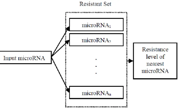
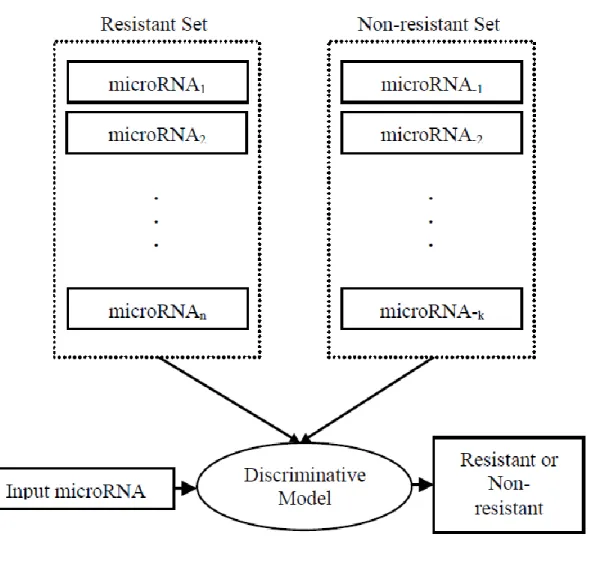
The pairwise approach takes an input microRNA and compares it with the other microRNAs in the resistant set of the drug under consideration. The comparison is made through the alignment of their mature sequences. Then, the model uses the annotations of the microRNA that has the highest alignment score to predict the resistance level of the input microRNA (Figure 1). Since it is already known that the regulatory behaviors of
13
microRNAs are guided by their mature sequences [16], we may reasonably expect a similarity between matures sequences of two microRNAs that give resistance to same chemotherapy drug.
Pairwise alignment in biological sequence analysis is basically used for finding sequence similarities in sequences in such a way that high sequence similarity implies crucial structural and functional similarity between sequences. Sequence analysis is simply a procedure of comparing two or more sequences by looking for a series of individual characters or patterns combined from characters that have the same order in sequences. Pairwise alignment of sequences takes two sequences and compares individual characters or patterns between them to find some similarities.
The aim in this study to use sequence analysis is to predict the relations between chemotherapy resistance and microRNA sequences. To solve that problem, it is needed to find the ‘best’ alignment between two sequences that are the mature sequences of the microRNA with known resistance and the microRNA that will be tested. To do that, we need a method for scoring alignments and an algorithm to find the alignment that has the ‘best’ score. The alignment score is found by dynamic programming algorithm using matrix and gap penalties [26]. Dynamic programming is also an efficient way of finding an optimal alignment score for relatively short sequences. Since microRNA mature sequences are of 22-25 nucleotides length, in this context, using a dynamic programming technique is a reasonable choice. Alignment by using dynamic programming ensures that the resulting alignment is optimal while it provides a cost effective solution [26].
To predict chemotherapy resistance of an input microRNA, we first perform a dynamic programming based local alignment between the input and other microRNAs in the training set. Then, most similar microRNA is selected to annotate the input such that their chemotherapy resistance is same. In other words, if the most similar microRNA is resistant, the query is also predicted as ‘resistant’.
14
Figure 1 Pairwise model for predicting microRNA resistance to a certain chemotherapy drug
2.3. Generative Method
2.3.1. VLMC - Variable Length Markov Chains
Sequence classification and clustering is complex, important and has significance in bioinformatics field. Attaining a training set of sequences, and fitting them with a generative probabilistic model that captivates statistical correlativity from the sequences in the set [27]. Variable length Markov chains gives us a capability to model a selected set of sequences or contexts that can have different lengths [27]. Variable length Markov chains (VLMM) are also powerfully capable of optimizing memory length locally within a model, and that special quality of VLMC’s ability capture the long term dependencies of some parts of the sequences and short term dependencies of the sequences [28]. Although n-th order Markov models are used to model the memory of fixed lengths, VLMMs are used for modeling the processes that has the varying memory length. That feature helps us about optimizing the length of memory that is needed locally.
15
Variable length Markov chains are sort of Markov chains that also have a structure that memories of chains depend on a variable number of lagged or delayed values [29]. For an input mature sequence S, indexed between 1 and N its likelihood for a specific VLMC is given by;
(1)
Where Lj is the optimal length of preceding subsequence and 1 j L j j
s
is that subsequence [30].2.3.2. PST – Probabilistic Suffix Trees
A probabilistic suffix tree is an efficient data structure to implement VLMC. The probabilistic suffix tree was proposed firstly by ‘Ron’, ‘Singer’ and ‘Thishby’ in 1996 as ‘probabilistic suffix automata’ [31]. The aim to propose this method was creating a new learning method. This method is used by many fields such as pattern recognition, machine learning. Its first usage in bioinformatics is classifying the protein families [32]. Probabilistic suffix trees had several variations to be used for protein sequencing. Biological probabilistic suffix tree approach was proposed by ‘Bejenaro’ and ‘Yona’ [33] which stands for a type of several probabilistic suffix models.
Probabilistic suffix tree is an index-based suffix tree storing the probabilistic values regarding to the subsequences and using probabilistic models [33]. It can be said that this method is based on the characteristic named ‘short memory’ that is common in biological sequences. Before probabilistic suffix tree is proposed, Markov chains and Hidden Markov models were used for modeling the sequences. However, both Markov chain and Hidden Markov model have some restrictions in their practical usage. Markov chain grows exponentially regarding of the length, because of that the less length Markov chains can work efficiently. In Hidden Markov model, the learning difficulty problem occurs.
N j j L j j L j j j N j js
S
s
S
P
S
P
1 1 1 1)
(
|
)
(
16
Therefore, there was a need for a new probabilistic learning model to get rid of the restrictions. Although probabilistic suffix tree has some restrictions like learning difficulty, it can be used efficiently on more length sequences. Probabilistic suffix tree was used firstly in 2000 by ‘Bejenaro’ and ‘Yona’ for classification of protein sequences.
“A PST over an alphabet is a non-empty tree, whose nodes vary in degree between zero (for leaves) and the size of the alphabet” [34]. The tree is composed from nodes and edges, and each is marked by a single symbol or the character from the alphabet that the probabilistic suffix tree is applied on and any symbol or character cannot be used more than one in the edges, which ensures that the degree of nodes are same and the bounded by the alphabet that the probabilistic suffix tree applied on. Since edges are marked or labeled by a character or a symbol, nodes are marked by strings that can be generated from that node to the root. Nodes also contain probability distribution vectors regarding to the alphabet. These probability distribution vectors act a significant role in predicting important subsequences or the patterns in strings.
The difference between the suffix trees and the probabilistic suffix trees is the structuring direction.
17
Take the above simulation as an example, in the suffix tree model when the symbol ‘k’ is added to the root, the first node is demonstrated as ‘k’, then after adding the symbol ‘l’, the second node is demonstrated as ‘lk’. However in the probabilistic suffix tree model, when the symbol or the character ‘k’ is added to the root, the first node is demonstrated as ‘k’, then after adding the symbol or the character ‘l’, the second node is demonstrated as ‘kl’. The difference between suffix trees and the probabilistic suffix trees is about structuring direction.
18
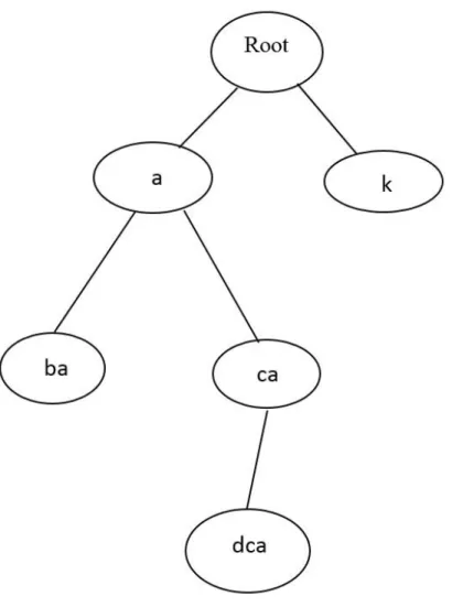
An example of a probabilistic suffix tree is given in the Figure 3. This example is constructed on the alphabet = {a, b, c, d, k}. The probability distribution vectors of nodes are given that (.2 , .2 , .2 , .2 , .2) is the probability distribution vector of the root node, (.05 , .5 , .15 , .2 , .1) is the probability distribution vector of the node that has ‘a’ in it, (.6 , .1 , .1 , .1 , .1) is the probability distribution vector of the node that has ‘k’ in it, (.05 , .4 , .05 , .4 , .1) is the probability distribution vector of the node that has ‘ba’ in it, (.05 , .25 , .4 , .25 , .05) is the probability distribution vector of the node that has ‘ca’ in it, and (.1 , .1 , .35 , .35 , .1) is the probability distribution vector of the node that has ‘dca’ in it. The probabilistic distribution vector of the node demonstrates the probability distribution over the next symbol. For instance, the probability distribution of the node that contains ‘ca’ as a substring is 0.05 for the symbol ‘a’, 0.25 for the symbol ‘b’, 0.4 for the symbol ‘c’, 0.25 for the symbol ‘d’ and 0.05 for the symbol ‘k’ correspondingly.
∑ is the symbol that demonstrates the alphabet to construct a probabilistic suffix tree. The alphabet can be amino acids that have 20 different types of amino acids, or the nucleotides of DNA or RNA that are adenine, guanine, cytosine, thymine or adenine, guanine, cytosine, uracil correspondingly.
𝑟1, 𝑟2, 𝑟3… … … 𝑟𝑛 𝑎𝑟𝑒 𝑡ℎ𝑒 𝑠𝑎𝑚𝑝𝑙𝑒 𝑠𝑒𝑡𝑠 𝑜𝑓 𝑛 𝑠𝑡𝑟𝑖𝑛𝑔𝑠 𝑜𝑣𝑒𝑟 𝑡ℎ𝑒 𝑎𝑙𝑝ℎ𝑎𝑏𝑒𝑡
𝑖 𝑖𝑠 𝑡ℎ𝑒 𝑖𝑛 𝑡ℎ𝑒 𝑟𝑎𝑛𝑔𝑒 𝑜𝑓 [1 , 𝑚] 𝑎𝑛𝑑 𝑟𝑖 = 𝑟
1𝑖𝑟2𝑖𝑟3𝑖… … … 𝑟𝑚𝑖
Then, the empirical probability is defined over a subsequence ‘s’. The empirical probability is defined in a way that the number that the subsequence is observed in the sample set is divided by the maximum number of occurrences of a pattern with the same size. Let ‘l’ defines the length of the subsequence ‘s’;
19
𝑋𝑠𝑖 ,𝑗= {1 , 𝑖𝑓 𝑠1𝑠2𝑠3… … … 𝑠𝑙= 𝑟𝑗𝑖𝑟𝑗+1𝑖 𝑟𝑗+2𝑖 … … … 𝑟𝑗+𝑙−1𝑖
0 , 𝑜𝑡ℎ𝑒𝑟𝑤𝑖𝑠𝑒
The actual empirical probability is related to the number of occurrences of “s” in the sample set of sequences. After defining the empirical probability, conditional empirical probability of a symbol that is the next symbol or right after the sequence. It is also defined in a way that the number of occurrences that the desired symbol is next to the given sequence or right after the given sequence divided by the total number of occurrences in the sequence.
2.3.2.1. PST Building
The length of the PST, memory length of the PST, is defined as the starting point in the PST construction process. The length can be the maximum length of a string that will be shown in the tree. Given an empirical probability threshold, sequences of length 1 through the length of the sequence is constructed in a probabilistic suffix tree up to reaching the empirical probability threshold or up to reaching to the maximal length boundary to the sequence. Empirical probability threshold is demonstrated as Pmin and it is responsible
for avoiding the exponential growing. As explained above in the probabilistic suffix tree part, Markov chains and Hidden Markov models have disadvantages about exponentially growing and the probabilistic suffix tree solves the problem by using the empirical probability threshold demonstrated as Pmin.
Constructing a probabilistic suffix tree starts with defining a root node. Then for every subsequences of the sequence, the empirical probability of observing the symbol that is next to the sequence or right after to the sequence is checked, and if the checked empirical probability is not negligible and if it is also importantly have different value from the empirical probability value of observing that symbol next to the sequence or right after to the sequence that is derived from removing the leftmost character of the subsequence, the subsequence is added to the PST [35]. The steps processed on the subsequences to be added to the PST is called pruning. In addition to the adding process, if the prediction function of a leaf node is identical or similar to its parent node’s prediction
20
function, then the leaf node is considered as useless. This also prevents the having almost identical or similar nodes in a PST.
The PST constructing process on a sample set includes five parameters. They are memory length as ‘L’, empirical probability threshold or the minimal probability as ‘Pmin’,
the difference measured between the parent node and the current node as ‘r’, the smoothing factor as γmin, and the α parameter that is used together with the smoothing
factor to define the threshold probability. Smoothing process assures that symbols will not have zero probabilities. γmin defines the minimum probability value of a symbol or the
character, and also the empirical probability values need to satisfy the smoothing factor.
2.3.2.2. Prediction with PST
For a given string called ‘s’, the prediction process of it using a probabilistic suffix tree is done character by character or symbol by symbol. It is done by “calculating the probability of each character or symbol by scanning the tree in search of the longest suffix that appears in the tree and ends just before that letter” [35]. Then, the conditional probability of that character or the symbol is given by the probability distribution associated with the corresponding node in the PST [35].
2.3.2.3. The Complexity of PST
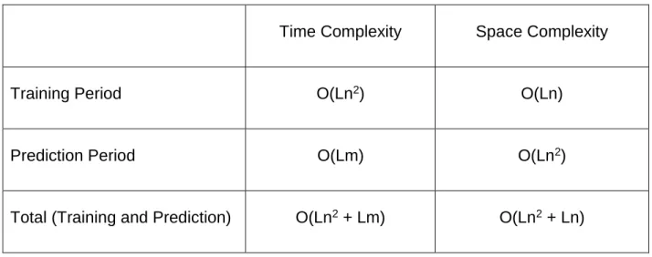
“Denote the length of the training set by n, the depth bound on the resulting PST by L, and the length of a generic query sequence by m. In these terms, the learning phase of the algorithm can be bounded by O (Ln2) time and O (Ln) space, as there may be O (Ln)
different subsequences of lengths 1 through L, each of which can be searched for, in principle, in time proportional to the training set length, while each contributes but a single node beyond its father node to the resulting structure” [35]. Given the length of the training set is ‘n’, and the depth of the PST is ‘L’, and the sequence length is ‘m’, the complexity of training and the prediction periods are given in the Table-3.
21
Table 3 Time and Space Complexity of the PST processes
Time Complexity Space Complexity
Training Period O(Ln2) O(Ln)
Prediction Period O(Lm) O(Ln2)
Total (Training and Prediction) O(Ln2 + Lm) O(Ln2 + Ln)
2.3.2.4. Generative Chemotherapy Resistance Prediction
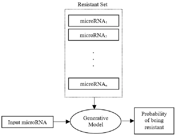
The generative approach that we consider here to predict chemotherapy resistance takes the set that has the microRNAs that are resistant to the corresponding to chemotherapy drug, and calculates a probabilistic model of generating those microRNA sequences in the same resistance characteristics. The model predicts the resistance level for an unknown input microRNA based on its probability of being generated from that model (Figure 4). The intuition behind this scheme is to infer the main sequential characteristics that may lead to resistance of microRNAs to given chemotherapy drug.
Owing to the sequential nature of our data, we adopt here a Markov model to build a probabilistic generative model for each chemotherapy drug. Because of the computational and storage limitations of Markov Chain of order L and the need for an excessive number of learning parameters for Hidden Markov Models, we use Variable Length Markov Chain in this context. Because its storage cost is less and performance is better [36], PSTs are used in this approach to implement VLMC for predicting the relations between chemotherapy resistance and microRNA sequences. The method is based on finding and identifying a set of significant patterns in microRNA sequences corresponding to chemotherapy chemicals. VLMC enables us to calculate the likelihood of whole
22
sequence for corresponding drug by simply multiplying local probabilities [30]. We simply compare the likelihood of an input microRNA being resistant or not to identify its class.
Figure 4 Generative model for predicting microRNA resistance to a certain chemotherapy drug.
2.4. Discriminative Method
2.4.1. Feature extraction
Feature extraction is the technique that is used for diminishing the quantity of resources that are required to be set of data by analyzing the data and clustering and grouping them according to some characteristic specialties. Feature extraction is populously used in the machine learning, image analysis, pattern recognition, data mining and business intelligence areas.
23
Feature extraction basics are described by Guyon and Elisseeff as predictive modelling, feature construction and feature selection [37]. The machine learning process is about encountering relationships between the patterns among the training examples, the predictive modelling is about the categorization or the determining the classification technique [37]. Feature construction is also described as preprocessing that includes standardization, normalization, signal enhancement, extraction of local features, linear and non-linear space embedding methods, non-linear expansions and feature discretization methods according to Guyon and Elisseeff [37]. Feature construction is also considered as one of the keys steps in the data analyzing process [37].
Feature selection, also variable selection, attribute selection, is basically selecting subsets from the pertinent big set of data.
Figure 5 Clustered objects
Figure 5 includes three clusters that contains groups of points that are clustered or classified with some specific characteristics. Feature extraction is the key and main process in the classification process.
24
2.4.2. Support Vector Machines (SVM)
Machine learning is widely used to identify structural patterns, groups from the data. We need to have training sets and some prediction models for computer to predict the class of an object. The system needs to generalize the objects for a given and previously seen and recognized set and needs to find an appropriate cluster or group for the new object. The computer can learn the recognition by a function that performs well in the given set that is also named the training set. Empirically, there is also chance to do it in the wrong way and it generates a ‘training error’. There is also an overall risk that can be caused from many functions used for the recognition, called ‘the test error’. In order to get a sufficient result, we also need to minimize the test error. Vapnik and Chervonenkis reported that there is an upper bound for the testing error is less than or equal to the summation of training error and the complexity of the models [38].
Test Error ≤ (Training Error) + (Complexity of the Models) (2)
Then, we need to have a function that is going to minimize the summation of the ‘training error’ and the ‘complexity of the models’. Then, the support vector machines becomes one ıf the solution for this minimization problem.
Support vector machines (SVM) is a supervised learning algorithms that are widely used in regression methods, clustering and classification. Classification of images and objects, text recognition, biological areas are the major areas that the support vector machine algorithms widely used. The first and the original support vector machine, known as linear classification, algorithm was reported by Vapnik and Chervonenkis. SVM is grouped into two main categories that are linear SVM and non-linear SVM.
The LibSVM library of the Weka, Waikato Environment for Knowledge Analysis, software is used in this thesis and results for each chemical is collected as ROC values.
25
2.4.3. Locally Weighted Learning (LWL)
Locally weighted learning algorithms (LWL) are a form of memory based learning algorithms and lazy learning algorithms. Lazy learning algorithms can be described as delaying the processing of the training data until a process query needs to be processed or answered [35]. Locally weighted learning is a set of function or method approximation techniques that the prediction is processing by using approximated local models that are around the interested points [39]. The main goal of the function or the method approximation is to recognize or find relationships between the inputs and outputs. In supervised learning processes, inputs are associated with the outputs, specifically one input for one output, in order to constitute a model that predicts some values that are used to estimate the closeness to the true modeling function [39]. Locally weighted algorithms are prediction methods that are done by local functions on some subsets of data, instead of using global functions on sets of global data. In other words, the LWL algorithms is about building local models for the whole function sets instead of building global models [39]. As mentioned above, LWL is a form of a lazy learning because it is characteristic that is delaying the training data until a query needs to be answered. This characteristic makes LWL algorithms more accurate approximation function
2.4.4. Discriminative chemotherapy resistance prediction
We adapt in this thesis the discriminative approach to predict chemotherapy resistance such that it uses two sets of microRNAs that are resistant to its corresponding chemotherapy chemical and non-resistant to its corresponding chemotherapy chemical. Discriminative model learns a separating decision function for resistant and non-resistant sequence features. The trained model predicts the resistance level of the input microRNA based on that function (Figure 6). Here, we consider two alternative methods for training a discriminative model; Support Vector Machine (SVM) and Locally Weighted Learning (LWL).
SVM is a powerful machine learning tool that we consider to classify microRNA sequences. An SVM classifier is generated by a two-step procedure: first, the high
26
dimensional input space of the SVM is non-linearly mapped into a higher dimensional feature space. In the second step, a linear hyper-plane is constructed in this feature space with the largest possible margin separating the classes of the data. The points classified by SVM are of two types: support vectors and non-support vectors. Non-support vectors are perfectly classified by the hyper-plane and are located outside of the separating margin. The parameters of the SVM do not depend on them, even if their positions are changed, provided that these points will stay outside the margin. The major advantage of the SVM classification is its better generalization ability owing to the fact that it finds the separating hyper plane with the largest margin using support vectors, as opposed to Neural Networks, at which all possible hyper-planes are evaluated. Thus, SVM is considered to be less prone to over fitting than other classifiers.
Our second option for machine learning classifier is the LWL algorithm that incorporates the idea of localization [35]. The main idea of localization is to assign a weight to each training observation that regulates its influence on the training process. This weight depends upon the location of the training point in the input variable space relative to that of the point to be predicted. Weights are bigger for the data points that are closer to the data you are trying to predict, thus 'local' in the name. While instance-based classifiers are often successful in linearly separable case of input data, when the data set is not linear, these methods tend to under fit the training data. The local approach here alleviates this problem by assigning weights to training data. Weighting the data can also be viewed as replicating relevant instances and discarding irrelevant instances.
A machine learning classifier, either SVM or LWL requires that the input must be a fixed length vector. Since the sequences that we study here are naturally of different lengths, we need to have an encoding scheme to represent them in a fixed length vector. Here, we use a common representation based on k-mer frequencies. A k-mer frequency refers to the frequency of appearance of a word with a length of k inside the sequence. In our case, the RNA alphabet is composed of 4 types of nucleotides: A, G, C, U. Therefore,
1-mer representation includes the frequencies of 4 nucleotide elements in mature
27
𝑆1 = {𝑝1 , 𝑝2 , 𝑝3 , 𝑝4 } (3)
Where pi corresponds to frequency of Adenine, Guanine, Cytosine, or Uracil.
2-mer representation of them in the microRNAs’ mature part takes 16 (4*4) vectors:
𝑆2 = {𝑝1𝑝1 , 𝑝2 𝑝2 , 𝑝3 𝑝3, 𝑝4𝑝4, … } (4)
3-mer representation of them in the microRNAs’ mature part takes 64 (4*4*4) vectors:
𝑆3 = {𝑝1𝑝1𝑝1, 𝑝2 𝑝2 𝑝2 , 𝑝3 𝑝3𝑝3 , 𝑝4𝑝4 𝑝4, …} (5) We integrate three k-mer representations for k=1,2, and 3 to build a single feature vector having a length of 84. We use then these vectors to feed SVM or LWM classifiers.
28
29
3. RESULTS
3.1. Data Sets
We used the database named CREAM – Chemotherapy Resistance Associated MiRSNP Database- that is free and online database including the microRNAs associated with 432 different chemotherapy resistances [40]. The dataset contains 1921 different microRNAs with resistance labels. Mature microRNA sequences were obtained from miRBase database [41]. Each entry in the database represents the microRNA and its corresponding mature sequences.
3.2. Experimental Setup and Evaluations
The evaluation criteria of this paper are based on ROC scores that are evaluated from ROC (Receiving Operating Characteristics) curves. ROC score was calculated from the area under the ROC curve. ROC analysis investigates and employs the relationship between sensitivity and specificity of a binary classifier. Sensitivity or true positive rate measures the proportion of positives correctly classified; specificity or true negative rate measures the proportion of negatives correctly classified. Conventionally, the true positive rate ‘tpr’ is plotted against the false positive rate ‘fpr’ [42]. All the experimental results in this paper collected as ROC scores in the [0 - 1] scale. A higher value of ROC score indicates a better prediction result where a ROC score is between 0 and 1 and the value 1 represents the perfect prediction.
We compiled the pairwise approach with dynamic- programming-based alignment, the generative model with VLMC, the discriminative model with SVM and LWL in the same experimental setup on the described data set. The methods were referred as "Pairwise", "Generative", "Discriminative (SVM)", and "Discriminative (LWL)" respectively. A ROC score was calculated from by the area that is under the ROC curve that is associated to each specific chemical.
In the pairwise method, the maximum value with the closeness to the high scored value and the maximum value with the closeness to the highest second scored value are
30
calculated. The average ROC value of the first scenario is found as 0.7203 and the average ROC value of the second scenario is found as 0.6581.
In the generative method, the ROC values are calculated by using the data structure type named probabilistic suffix trees, and two different scenario was applied. First scenario is using a probabilistic suffix tree with depth 3, and the second scenario is using a probabilistic suffix tree with depth 5.
In the discriminative method, support vector machines (SVM) and locally weighted learning (LWL) algorithms were used in the process. 3-mer and 2-mer forms of pyrimidine in the sequences were both used in the process.
The ROC algorithm that is depicted below as Algorithm-1 was applied to the results to calculate the ROC values of each method.
Inputs: ‘L’ is defined as the closest value to the set (set of tags), and the ‘tag’ is defined as a tag that can be 0 for false, and 1 for true.
Output: ‘R’ is defined as the ROC value.
Algorithm-1 Calculation of Roc value
/∗ 𝑎𝑠𝑠𝑖𝑔𝑛𝑖𝑛𝑔 𝑖𝑛𝑖𝑡𝑖𝑎𝑙𝑖𝑧𝑎𝑡𝑖𝑜𝑛 𝑣𝑎𝑙𝑢𝑒 𝑡𝑜 ‘𝑡𝑟𝑢𝑒 𝑝𝑜𝑠𝑖𝑡𝑖𝑣𝑒𝑠’ ∗/ 𝑡𝑝 −> 0 /∗ 𝑎𝑠𝑠𝑖𝑔𝑛𝑖𝑛𝑔 𝑖𝑛𝑖𝑡𝑖𝑎𝑙𝑖𝑧𝑎𝑡𝑖𝑜𝑛 𝑣𝑎𝑙𝑢𝑒 𝑡𝑜 ‘𝑓𝑎𝑙𝑠𝑒 𝑝𝑜𝑠𝑖𝑡𝑖𝑣𝑒𝑠’ ∗/ 𝐹𝑝 −> 0 /∗ 𝑎𝑠𝑠𝑖𝑔𝑛𝑖𝑛𝑔 𝑖𝑛𝑖𝑡𝑖𝑎𝑙𝑖𝑧𝑎𝑡𝑖𝑜𝑛 𝑣𝑎𝑙𝑢𝑒 𝑡𝑜 𝑡ℎ𝑒 𝑅𝑂𝑉 𝑣𝑎𝑙𝑢𝑒 ∗/ 𝑅 −> 0 /∗ 𝑓𝑖𝑛𝑑𝑖𝑛𝑔 𝑡ℎ𝑒 𝑣𝑎𝑙𝑢𝑒𝑠 𝑜𝑓 𝑡𝑟𝑢𝑒 𝑝𝑜𝑠𝑖𝑡𝑖𝑣𝑒𝑠 𝑎𝑛𝑑 𝑓𝑎𝑙𝑠𝑒 𝑝𝑜𝑠𝑖𝑡𝑖𝑣𝑒𝑠 𝑓𝑜𝑟 𝑒𝑎𝑐ℎ 𝑒𝑙𝑒𝑚𝑒𝑛𝑡 𝑖𝑛 𝑡ℎ𝑒 𝑠𝑒𝑡 ‘𝐿’ ∗/ 𝑓𝑜𝑟 𝐿 𝑎𝑠 𝑡𝑎𝑔
31 𝑖𝑓 𝑡𝑎𝑔 = 1 𝑡𝑝 −> 𝑡𝑝 + 1 𝑒𝑙𝑠𝑒 𝑓𝑝 −> 𝑓𝑝 + 1 𝑅 −> 𝑅 + 𝑡𝑝 𝑒𝑛𝑑 𝑖𝑓 𝑒𝑛𝑑 𝑓𝑜𝑟 /∗ 𝑐𝑎𝑙𝑐𝑢𝑙𝑎𝑡𝑖𝑜𝑛 𝑜𝑓 𝑡ℎ𝑒 𝑅𝑂𝐶 𝑣𝑎𝑙𝑢𝑒 𝑎𝑐𝑐𝑜𝑟𝑑𝑖𝑛𝑔 𝑡𝑜 𝑡ℎ𝑒 𝑡𝑟𝑢𝑒 𝑝𝑜𝑠𝑖𝑡𝑖𝑣𝑒 𝑣𝑎𝑙𝑢𝑒𝑠 𝑎𝑛𝑑 𝑓𝑎𝑙𝑠𝑒 𝑝𝑜𝑠𝑖𝑡𝑖𝑣𝑒 𝑣𝑎𝑙𝑢𝑒𝑠 ∗/ 𝑖𝑓 𝑡𝑝 = 0 𝑅 −> 0 𝑒𝑙𝑠𝑒 𝑖𝑓 𝑓𝑝 = 0 𝑅 −> 1 𝑒𝑙𝑠𝑒 𝑅 −> 𝑅/𝑡𝑝 ∗ 𝑓𝑝 𝑒𝑛𝑑 𝑖𝑓 𝑒𝑛𝑑 𝑖𝑓 3.3. Empirical Results
All of the ROC value results are listed in the Table-5. The first column represents the names of the columns. For each chemical, the ROC values of SW-1, SW-2, 3, PST-5, 3-MER-SVM, 3-MER-LWL, 2-MER-SVM, 2-MER-LWL that are correspondingly stands
32
for SW alignment with one maximum value, SW alignment with two maximum values, probabilistic suffix tree with depth equals 3, probabilistic suffix tree with depth equals 5, support vector machine that is applied on the 3-mer structure of pyrimidine, support vector machine that is applied on the 3-mer structure of pyrimidine, support vector machine that is applied on the dimer structure of pyrimidine, locally weighted learning that is applied on the 3-mer structure of pyrimidine, locally weighted learning that is applied on the dimer structure of pyrimidine.
According to Table-4, the average values for all the methods are following: Table 4 Average ROC values of the methods
Approach Minimum Maximum Average
Pairwise (SW_1) 0.567 0.875 0.719 Pairwise (SW_2) 0.416 0.815 0.656 Generative (PST_3) 0.323 0.728 0.483 Generative (PST_5) 0.323 0.728 0.483 Discriminative 3-mer (LWL) 0.430 0.730 0.570 Discriminative 3-mer (SVM) 0.418 0.730 0.555 Discriminative 2-mer (LWL) 0.435 0.766 0.557 Discriminative 2-mer (SVM) 0.421 0.672 0.509
33
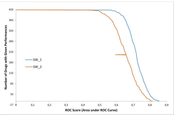
3.3.1. Pairwise method
In the pairwise method, the maximum value with the closeness to the high scored value and the maximum value with the closeness to the highest second scored value are calculated. The average ROC value of the first scenario is found as 0.7203 and the average ROC value of the second scenario is found as 0.6581.
In the Figure 7, the ROC values are demonstrated. The x-axis stands for the chemicals, each chemical has an exact number, and the y-axis stands for the ROC values that is in the range of [0, 1].
Figure 7 The ROC values of the Pairwise Methods
3.3.2. Generative method
In the generative method, the ROC values are calculated by using the data structure type named probabilistic suffix trees, and two different scenario was applied. First scenario is
-17 33 83 133 183 233 283 333 383 433 0 0,1 0,2 0,3 0,4 0,5 0,6 0,7 0,8 0,9 N u m b e r o f D ru gs wi th G iv e n Pe rfor m an ce s
ROC Score (Area under ROC Curve)
SW_1 SW_2
34
using a probabilistic suffix tree with depth 3, and the second scenario is using a probabilistic suffix tree with depth 5.
However, the results taken from the scenario with depth 3 and scenario with depth 5 are same. In the Figure 8, the ROC values are represented. The x-axis stands for the chemicals, each chemical has an exact number, and the y-axis stands for the ROC values that is in the range of [0, 1].
Figure 8 The ROC values of the Generative Methods
-17 33 83 133 183 233 283 333 383 433 0 0,1 0,2 0,3 0,4 0,5 0,6 0,7 0,8 N u m b e r o f D ru gs wi th G İv e n Pe rfor m an ce
ROC Score (Area Under ROC Curve)
35
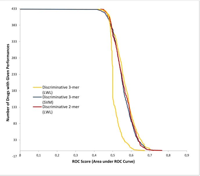
3.3.3. Discriminative method
In the discriminative method, support vector machines (SVM) and locally weighted learning (LWL) algorithms were used in the process. 3mer and 2mer representations of nucleotides in the sequences were both used in the process.
3mer SVM, 3mer LWL, 2mer SVM and 2merLWL Roc results were calculated and shown in the Figure 9.
Figure 9 The ROC values of the Discriminative Methods
-17 33 83 133 183 233 283 333 383 433 0 0,1 0,2 0,3 0,4 0,5 0,6 0,7 0,8 0,9 N u m b e r o f D ru gs wi th G iv e n Pe rfor m an ce s
ROC Score (Area under ROC Curve)
Discriminative 3-mer (LWL) Discriminative 3-mer (SVM) Discriminative 2-mer (LWL)
36
3.3.4. Comparison
We compiled the pairwise approach with dynamic- programming-based alignment, the generative model with VLMC, the discriminative model with SVM and LWL in the same experimental setup on the described data set. The methods were referred as "Pairwise", "Generative", "Discriminative (SVM)", and "Discriminative (LWL)" respectively. A ROC score was calculated from by the area that is under the ROC curve that is associated to each specific chemical. Figure 10 depicts the number of chemotherapy drugs with the given ROC score performance for each methodology applied.
Figure 10 Comparison of methods shown by number of drug labels with given Area under ROC performance
As shown, the best accuracy was achieved by pairwise model. The highest ROC score is 0.875 with this method. In the worst case, this method attained a ROC score of 0.567. For the generative approach, the minimum and maximum ROC scores are 0.323 and 0.728 respectively.
37
4. CONCLUSION
We study the problem of predicting the resistance of a microRNA to a chemotherapy treatment through a certain chemical drug. To this end, we consider solely mature sequence to assign given microRNA to resistant or non- resistant class for a chemotherapy chemical under consideration. Among three different computational approaches we considered, we obtained the best results with the pairwise approach where generative and discriminative models produced almost random solutions on an experimentally validated dataset. These results determine that the microRNAs which are commonly resistant to a specific chemotherapy chemical do not necessarily have similar sequential characteristics in their mature parts. On the other hand, a high similarity between any two microRNA mature sequences may imply a similar behavior in their resistance to certain chemotherapies. The lower accuracies achieved with generative and discriminative approach can be attributed to the fact that 2-mer or 3-mer encoding schemes cannot be biologically representative for microRNAs to be resistant to a certain chemotherapy or not.
This is the first study that evaluates the predictability of specific chemotherapy resistance of microRNA using only sequence information. The results promote the use of pairwise techniques as a complementary tool in association studies for microRNAs and drugs in clinical environments. Future work includes the consideration of problem-specific sequence similarity measures instead of using general-purpose dynamic programming algorithms for alignment.
38
REFERENCES
[1] H. Li and B. B. Yang, "Friend or foe: the role of microRNA in chemotherapy resistance.," Acta Pharmacologica Sinica 34.7, pp. 870-879, 2013.
[2] C. E. Jansen, C. Miaskowski, M. Dodd, G. Dowling and J. Kramer, "A metaanalysis of studies of the effects of cancer chemotherapy on various domains of cognitive function.," Cancer 104.10, pp. 2222-2233, 2005.
[3] D. He, F. Gu, F. Gao, J. Hao, D. Gong, X. Gu, A. Mao, J. Jin, L. Fu and X. Ma, "Genome-wide profiles of methylation, microRNAs, and gene expression in chemoresistant breast cancer."," Scientific Reports 6, p. 24706, 2016.
[4] I. Alvarez-Garcia and E. A. Miska, "MicroRNA functions in animal development and human disease.," Development 132.21, pp. 4653-4662, 2005.
[5] Z. Liu, A. Sall and D. Yang, "MicroRNA: an emerging therapeutic target and intervention tool.," International journal of molecular sciences 9.6, p. 978–999, 2008.
[6] A. Carè, "MicroRNA-133 controls cardiac hypertrophy.," Nature Medicine 13, pp. 613-618, 2007.
[7] E. A. Wiemer, "The role of microRNAs in cancer: no small matter.," Eur. J. Cancer.