Scheduling with tool changes to minimize total completion time

TS

ÍS J^S

*

C r8 é>

m e

minimizi

total

C O lFLlflO i TIME

TMESIS

SUBMITTED TO THS ВЕРАИТѢЖЧТ OF INDUSTRIAL.

ENGINE-ERIHG

AND THE INSTITUTE OF ENGîNESEïNG AND SGIENÏCE.S

OF BILKSNT UNIVERSITY

IN PARTIAL FULFILLMENT OF THE REQ

FOE THE DEGREE OF

MASTER OF SCIENCE

A THESIS

SUBMITTED TO THE DEPARTMENT OF INDUSTRIAL ENGINEERING

AND THE INSTITUTE OF ENGINEERING AND SCIENCES OF BILKENT UNIVERSITY

IN PARTIAL FULFILLMENT OF THE REQUIREMENTS FOR THE DEGREE OF

MASTER OF SCIENCE

^ v r iM DîolöM Gone;

/

4

Evrim Didem Güneş

December, 1998

İ99 S О

I certify that I have read this thesis and that in my opinion it is fully adequate, in scope and in quality, as a thesis for the degree of Master of Science.

^

Âkı.

Asst. Prof. M. Selim Aktürk(Principal Advisor)

I certify that I have read this thesis and that in my opinion it is fully adequate, in scope and in quality, as a thesis for the degree of Master of Science.

Assoc. Prof. Ömer Benli

I certify that I have read this thesis and that in my opinion it is fully adequate, in scope and in quality, as a thesis for the degree of Master of Science.

\

Asst. ^ o f . OyaTKkin Karaşan

Approved for the Institute of Engineering and Sciences:

Prof. Mehme^^^^ray

SCHEDULING W IT H TOOL CHANGES TO MINIMIZE

TO TAL COM PLETION TIM E

Evrim Didem Güneş

M.S. in Industrial Engineering

Supervisor: Asst. Prof. M. Selim Aktürk

December, 1998

In the literature, scheduling models do not consider the unavailability of tools. The tool management literature separately considers tool loading problem when tool changes are due to part mix. However in manufacturing settings tools are changed more often due to tool wear. In this research, the problem of scheduling a set of jobs to minimize total completion time on a single CNC machine is considered where the cutting tool is subject to wear.

We show that this problem is NP-hard in the strong sense. We discuss the behavior of SPT heuristic and show that its worst case performance ratio is bounded above by a constant. A pseudo-polynomial dynamic programming formulation is provided to solve the problem optimally. Furthermore, heuristic algorithms are developed including dispatching heuristics and local search algorithms. It is observed that the performance of SPT rule gets worse as the tool change time increases and tool life decreases. The best improvement over the SPT rule’s performance is achieved by the proposed genetic algorithm with problem space search.

Key words: Scheduling, Completion Time, Tool Management, Heuristics

KESİCİ

uç

DEĞİŞİMİ DURUM UNDA T O P L A M İŞ BİTİM

ZAM ANINI E N A ZL A M A K İÇİN ÇİZELGELEME

Evrim Didem Güneş

Endüstri Mühendisliği Bölümü Yüksek Lisans

Tez Yöneticisi: Yrd. Doç. M. Selim Aktürk

Aralık, 1998

Literatürdeki çizelgeleme modellerinde kesici uç kullanımında kısıt yoktur. Kesici uç işletim sistemi literatürü uç değişimi parça sırasına bağlı olduğunda kesici uç yükleme problemini ayrıca ele alır. Fakat üretim koşullarında kesici uçlar daha cok aşınmaya bağlı olarak değiştirilir. Bu çalışmada, kesici ucun aşınmaya maruz kaldığı tek bir CNC makinasinda bir grup işin toplam iş bitim zamanını enazlamak üzere çizelgelenmesi problemi ele alınmıştır.

Bu problemin kuvvetli anlamda NP-zor olduğu ve en kısa işlem süresi (EIS) kuralının en kötü durum performans oranının üstten bir sabitle sınırlı olduğu gösterilmiştir. Problemi eniyileyerek çözmek için bir sahte polinom dinamik programlama formülasyonu verilmiştir. Ayrıca, bazı hızlı sezgisel algoritmalar ve yerel tarama algoritmaları geliştirilmiştir. EIS kuralının performansının uç değiştirme zamani arttıkça ve uç kullanım ömrü azaldıkça kötüye gittiği gözlenmiştir. EIS kuralı üzerine en çok gelişmeyi problem uzayı taraması kullanan genetik algoritma sağlamiştır.

Anahtar sözcükler·. Çizelgeleme, İş Bitim Zamanı, Kesici Uç işletim Sistemi, Sezgisel Yöntemler.

I would like to express my sincere gratitude to Selim Aktiirk for his invaluable advises and encouragement during my graduate study. He has been guiding me with patience and everlasting interest not only for this research but also for my future career.

I am also indebted to Jay B. Ghosh for his great helps and guldence in all phases of this study. He has invaluable contribution to this theis.

I am grateful to Robert Storer for showing keen interest to the problem and helping for the solution methods.

I am also indebted to Ömer Benli and Oya Ekin Karaşan for showing keen interest to the subject matter and accepting to read and review this thesis.

I would like to thank to my friend Bora Uçar for his helps in C programming. I would like to express my deepest gratitude to Hande Yaman, for being with me in every field of life and giving me morale and academic support during six years in the university. I owe much to her friendship and solidarity. I am also grateful to my officemate Ayten Türkcan for continuously providing morale support to me. She gave me courage whenever I was desperate, and also helped me a lot for technical issues. I cannot forget the six years’ friendship of Deniz Özdemir and the morale support she provided even when she was far away. I am grateful to Senem Erdem for her sincere friendship and support, and the night calls, giving me relief in the hard times.

Finally, I want to thank to Gonca Yidirim, Banu Yüksel, Özgür Ceyhan, Seçil Gergün, Barış Ata, Emre Alper Yıldırım, Murat Özgür Kara, Füsun Atik, Özlem Özhan and my sister Elif for their friendship and encouragement for my studies.

1 Introduction 2 Literature Review

3 Problem Statement 14

3.1 Problem Definition and A s su m p tio n s... 15 3.2 Characteristics of the P ro b le m ... 17 3.2.1 Complexity of the P roblem ... 19 3.2.2 Performance of SPT Heuristic 22

3.2.3 Conditions for optimality of SPT 30

3.3 Summary 32

4 The Algorithms 34

4.1 Dynamic Programming A lgorith m ... 35

4.2 Heuristic Algorithms 38

4.2.1 Dispatching H e u r is tic s... 39

4.2.2 Knapsack H eu ristic... 45

4.2.3 Local Search A lg o rith m s ... 47

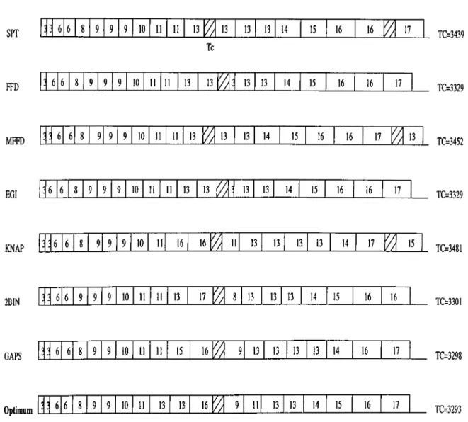
4.3 Example P r o b le m ... 52 ... 52 ... 53 ... 54 ... 55 ... 55 ... 56 ... 58 4.3.1 S P T ... 4.3.2 F E D ... 4.3.3 M F F D ... 4.3.4 Ranking Index EGI . 4.3.5 Knapsack Heuristic . 4.3.6 Two Bin Heuristic . 4.3.7 G A P S ... 5 Experimental Design 63 5.1 Experimental S e ttin g ... 63

5.2 Experimental R e s u lts... 66

5.3 S u m m a r y ... 73

6 Future Research Directions 75 6.1 Problem D e fin it io n ... 75

6.2 D iscu ssion ... 77

6.2.1 C a s e I : T c = 0 ... 78

6.2.2 Case II : T o 0 80 6.2.3 Further Issues for an Exact A l g o r i t h m ... 80

6.3 Summary 83

7 Conclusion

7.1 Results

7.2 Future Research Directions

84

. 84

. 86

Bibliography 87

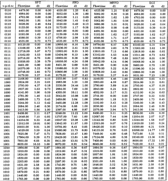
A Computational Results for 20 Jobs 91 B Computational Results for 50 Jobs 102

C Computational Results for 100 Jobs 113

3.1 Representation of a schedule as blocks of j o b s ... 17

3.1 Comparison of SPT performance with optimal v a l u e s ... 24

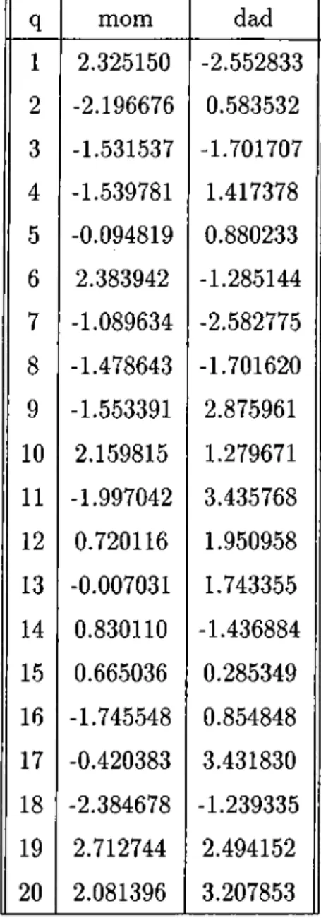
4.1 GAPS-The parent vectors chosen from the initial population . . 59

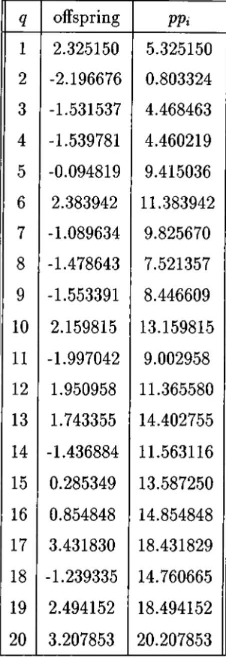
4.2 GAPS-child vector and corresponding perturbed processing times 60 4.3 GAPS-perturbed sequence converted to original d a t a ... 61

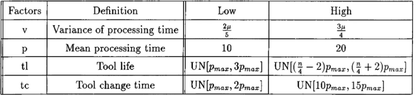
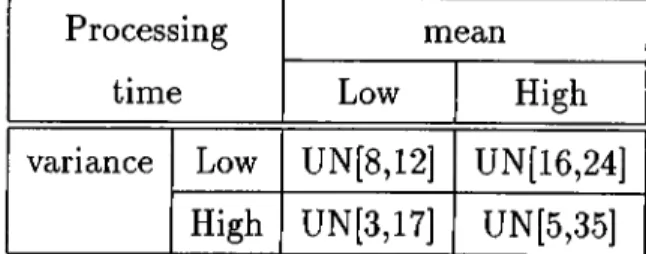
5.1 Experimental design f a c t o r s ... 64

5.2 Processing time distributions for different factor levels... 65

5.3 Summary results for the overall c o m p u ta tio n s ... 67

5.4 Average percent deviations (d l) for changing tl-tc factors . . . . 71

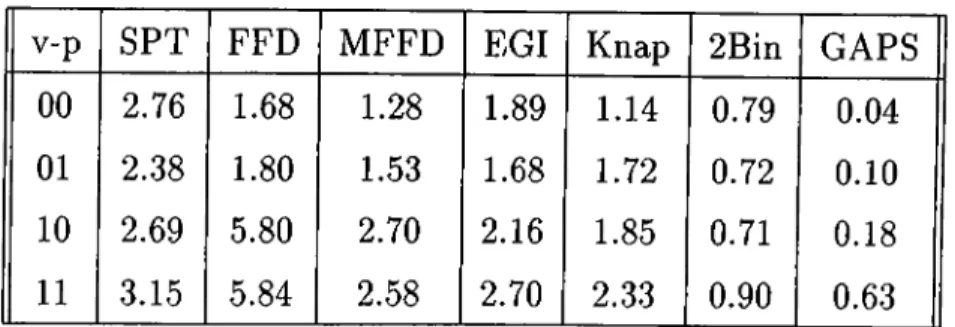
5.5 Average percent deviations (d l) for changing v-p factors . . . . 72

A .l Averages over ten replications for n = 2 0 ... 92

A .2 Averages over ten replications for n=20 (c o n tin u e d )... 92

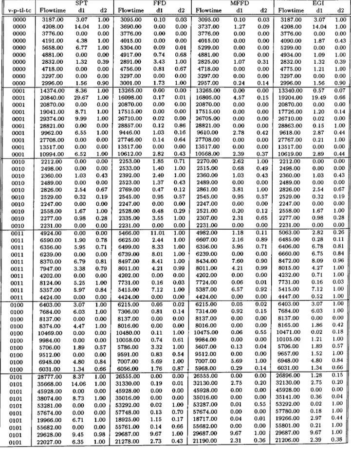
A.3 Computational results for SPT, FED, MEED, EGI algorithms for n = 2 0 ... 93

A .4 Computational results for SPT, FED, MFFD, EGI algorithms for n=20 (c o n tin u e d )... 94

A .5 Computational results for SPT, FFD, MFFD, EGI algorithms

for n=20 (c o n tin u e d )... 95

A .6 Computational results for Knap, 2Bin, GAPS algorithms for n=20 96 A .7 Computational results for Knap, 2Bin, GAPS algorithms for n=20 (c o n tin u e d )... 97

A .8 Computational results for Knap, 2Bin, GAPS algorithms for n=20 (c o n tin u e d )... 98

A .9 Computation times for n = 2 0 ... 99

A .10 Computation times for n=20 (co n tin u e d )...100

A. 11 Computation times for n=20 (c o n tin u e d )...101

B . l Averages over ten replications for n = 5 0 ... 103

B.2 Averages over ten replications for n=50 (c o n tin u e d )...103

B.3 Computational results for SPT, FFD, MFFD, EGI algorithms for n=50 ... 104

B.4 Computational results for SPT, FFD, MFFD, EGI algorithms for n=50 (c o n tin u e d )... 105

B.5 Computational results for SPT, FFD, MFFD, EGI algorithms for n=50 (c o n tin u e d )... 106

B.6 Computational results for Knap, 2bin, GAPS algorithms for n=50107 B.7 Computational results for Knap, 2Bin, GAPS algorithms for n=50 (c o n tin u e d )...108

B.8 Computational results for Knap, 2Bin, GAPS algorithms for n=50 (c o n tin u e d )...109

B.9 Computation times for n = 5 0 ... 110

B.IO Computation times for n=50 (co n tin u e d )... I l l B . l l Computation times for n=50 (c o n tin u e d )... 112

C . l Averages taken over 10 replication for n = 1 0 0 ... 114

C.2 Averages taken over 10 replication for n=100 (continued) . . . . 114

C.3 Computational results for SPT, FFD, MFFD, EGI for n=100 . 115 C.4 Computational results for SPT, FFD, MFFD, EGI for n=100 (continued) ... 116

C.5 Computational results for SPT, FFD, MFFD, EGI for n=100 (continued) ... 117

C.6 Computational results for Knap, 2Bin, GAPS algorithms for n = 1 0 0 ...118

C.7 Computational results for Knap, 2Bin, GAPS algorithms for n=100 ( c o n t in u e d ) ... 119

C.8 Computational results for Knap, 2Bin, GAPS algorithms for n=100 ( c o n t in u e d ) ... 120

C.9 Computation times for n = 1 0 0 ... 121

C.IO Computation times for n=100 (c o n t in u e d ) ... 122

Introduction

Scheduling has been an attractive field for researchers for a long time. It deserves this attention since scheduling is an important part of strategic planning in industry and has significant impact on all economic activities. The term scheduling can be defined as “the process of organizing, choosing and timing resource usage to carry out all activities/tasks necessary to produce the desired outputs at desired times, while satisfying a large number of time and relationship constraints among the activities and resources” [22]. In short, it is the allocation of scarce resources over time to a collection of tasks. Scheduling decisions in manufacturing organizations are associated with many cost terms. These are mainly related with customer satisfaction, such as tardiness costs, or investments into system resources as flowtime costs.

The manufacturing organizations have been using flexible manufacturing systems (FMSs) widely in recent years in order to be able to meet the diversified customer needs and compete in today’s world market. An FMS is mainly defined as a system dealing with high level distribution data processing and automated material flow using computer controlled machines, assembly cells, industrial robots, inspection machines and so on, together with computer integrated material handling and storage systems. Basically, it is a group of CNC machine tools interconnected by a material handling system and controlled by a computer system.

Tool management is the most dynamic and critical facility in FMSs and requires keen attention. The cutting tools used in FMSs are subject to wear and they have relatively short tool lives in the planning horizon. Moreover, the tool holding capacity of FMSs is limited, so the machine may not be able to carry all the required tools to complete the jobs. For this reason, one main task to accomplish for tool management is to find a scheduling strategy to account for tool availability and tool changes.

Scheduling activities are done considering different goals. Sometimes the customer satisfaction in terms of meeting the deadline is taken into account, which is reflected as the tardiness cost in the objective function of the scheduling problem. Another cost measure is the time a job spends in the system, defined as the fiowtime of the job. Flowtime cost is related with the investment into system resources and is reflected as the work in process inventories in the system. Minimizing the total flowtime is an important goal for scheduling activities considering the importance of maintaining low inventory levels for manufacturing firms.

In this study, a single CNC machine is considered, being a part of a flexible manufacturing system, and the scheduling problem with the objective of minimizing total flowtime is studied while also focusing on the tool management issue to cope with the tool changes due to tool wear. The existing studies in the literature ignore the interaction between the scheduling decisions and the tool change requirements due to tool wear. In the tool management literature, the tool changes are generally considered to be due to part mix, that is, due to different tooling requirements of the parts. The cost terms which are directly related with scheduling decisions such as flowtime of jobs are not included in the objective function. On the other side, the scheduling literature also does not consider the tool change requirements. There are few studies considering the resource unavailability, but they consider the resources as machines, and the unavailability is limited to occur for one time only.

As a result, the scheduling problem with tool changes due to tool wear is an untouched topic in the literature. In this study, we aim to show the

validity of this problem and try to find solution methods to fill in this gap in the literature. We study the simplest case of the joint tool management and scheduling problem in order to provide some insights to find a solution for the more general cases. The problem we consider is characterized by the following conditions: There are n jobs with predetermined processing times. There is ample tool of single type, which has a constant tool life and constant tool changing time. When the tool life is over, the tool has to be changed. We assume that a manufacturing operation cannot be interrupted for a tool change due to surface finish requirements.

At the beginning, we analyze the complexity of this problem and show that it is strongly NP-hard. Afterwards, we investigate the behavior of the well known shortest processing time (SPT) heuristic for this problem and show that its worst case performance is bounded above by a constant. Then, we discuss some conditions which would guarantee optimality of SPT rule.

Since our problem is NP-hard, it is justified to solve it by heuristic approaches. In this study, we provide a dynamic programming algorithm which is shown to be pseudo-polynomial. Furthermore, we develop several heuristic algorithms including dispatching heuristics and local search algorithms. We test the performance of the proposed algorithms on a set of randomly generated problems and discuss the results. We show that an improvement over the performance of the SPT heuristic is provided with the proposed algorithms.

We will also elaborate on an extension of this problem in order to provide insights for a possible future research. We consider to incorporate the determination of the machining parameters which would affect the processing times and the tool life into the scheduling problem with tool changes. This time the objective function would also include the manufacturing costs in addition to the flowtime cost.

The remainder of the thesis can be outlined as follows. In the following chapter, we give a short review of the literature on the scheduling problems with an availability constraint and tool management studies along with some studies on bin packing problem, which is related with our problem in some aspects. We

define the underlying assumptions, and give a list of notation in Chapter 3. In this chapter, we also discuss the characteristics of the problem and analyze the performance of the SPT heuristic for our problem providing some examples of interesting instances. We also investigate the worst case performance of SPT, and the conditions for optimality of this heuristic in this chapter. In Chapter 4, we explain the pseudo-polynomial dynamic programming formulation and the proposed heuristic algorithms in detail. Then, we illustrate these algorithms on a numerical example. In Chapter 5, we discuss the computational analysis done with these algorithms. The discussion on a possible extension of this problem is given in Chapter 6. Finally in Chapter 7, the concluding remarks of this study is provided with some suggestions for future research.

Literature Review

Research on manufacturing has been traditionally done in separate veins for tool management issues and scheduling problems. In both fields, extensive research has been done for modeling the systems, and developing control methods. However, the interaction between these two levels of manufacturing decision processes has not been addressed by the researchers.

Scheduling can be defined as the allocation of scarce resources over time to a collection of tasks. It is a decision-making process that exists in most manufacturing systems, and also in most information-processing environments which plays a crucial role in strategic planning. For this reason it has attracted the attention of researchers since the beginning of this century, with the work of Henry Gantt and other pioneers. Since than, considerable amount of theoretical work has been done concerning various different models. An excellent overview of deterministic scheduling can be found in the textbook by Baker [7]. A recent book by Pinedo [24] deals with both deterministic and stochastic models with applications to real world problems.

There are many costs to the system associated with the scheduling decisions. Among them the most commons are cost of completing the tasks after the due date, which is called the tardiness cost, and cost of tasks waiting to be completed, called the flowtime cost. Flowtime of a job is the time it spends

in the system. The cost of flowtime involves the investment into system resources, and is reflected as the inventory levels in the system. Especially with the emergence of new paradigms in production systems such as just in time philosophy, minimizing the inventory levels in the manufacturing environment gained importance. Consequently, the scheduling objective corresponding to this goal is minimizing the total flowtime. In this study, our objective will be minimizing the total flowtime.

Although the variety of different models studied in scheduling theory lies in a big range, there are still some deficiencies in the literature. The resources in scheduling theory are mostly considered as the machines, without referring to the tooling level. As discussed in Lee et al. [21] and Pinedo [24], most theoretical models do not take the unavailability of resources into account. It is usually assumed that the machine is available at all times. However in the real world, machines are usually not continuously available. Certainly, this observation is valid for the machine tools, and the unavailability of tools is a more common situation since the tools actually have short lives with respect to the planning horizon, as reported by Gray et al. [13].

In the literature, there are no studies considering the tool life and tool change time requirement due to tool wear, and incorporating them with scheduling objectives. However, there are some studies done in recent years considering the unavailability of machines. These problems have similar characteristics with the scheduling with tool changes problem.

The research on scheduling with availability constraint is mostly focused on machine breakdowns and maintenance intervals. The most common objective is minimizing the total flowtime. Adiri et al. [1] considered flowtime scheduling problem when machine faces breakdowns at stochastic time epochs, and repair time is also stochastic. The processing times are assumed constant. They have provided the NP completeness result of the problem, and showed that SPT minimizes expected total flowtime when times to breakdown are exponential. In the case of single breakdown and concave distribution function of the time to breakdown, they have again showed the stochastic optimality of SPT. They

have also analyzed the single deterministic breakdown case, and found a worst case performance bound for SPT heuristic, which was 5/4.

Lee and Liman [17] have also studied the same problem, but considered only deterministic single scheduled maintenance case. In this study, they have given a simpler proof of NP completeness, and found a better bound for SPT, being 9/7. They have also shown that this bound is tight.

There are also some studies on flowshop and parallel machine scheduling with an availability constraint. Lee and Liman [18] considered two machines in parallel scheduling problem of minimizing the total completion time where one machine is available all the time and the other machine is available from time zero up to a fixed point in time. They have given NP-completeness proof for the problem, and provided a pseudo-polynomial dynamic programming algorithm. Moreover, in this study, a heuristic is proposed which is based on a slight modification of SPT rule considering the capacity of the machine with availability constraint. This heuristic is shown to have an error bound of 0.50.

Lee [19] studied minimizing the makespan in the two-machine flowshop scheduling problem. The availability constraint applies for one of the machines. The NP hardness proof is done and a pseudo-polynomial dynamic programming formulation is provided in this study. In addition, he provides two heuristics with an error bound analysis, for problems with availability constraint on the first machine, and on the second machine.

In a companion paper, Lee [20] discusses the machine scheduling with an availability constraint in more detail. He analyses the problem for different performance measures such as makespan, total weighted completion time, tardiness, and number of tardy jobs, and for different machine environments such as single machine, parallel machines, and two machine flowshop. In each case, the complexity issue is discussed, and either a polynomial algorithm is provided, or the NP hardness proof is done. In case of NP completeness of the problem, pseudo-polynomial dynamic programming algorithms are developed to solve it optimally, and/or a heuristic with an error bound analysis is provided. In this study, two different cases are considered, which are resumable.

and nonresumable cases. A job is called resumable if it can be interrupted in case of an unavailability, and can be continued after machine is available again. In nonresumable case, the job has to be restarted rather than continue. The nonresumable case is similar to the tool change problem, since for surface finish quality considerations, we do not let the process on a job to be interrupted, and continued after a tool change.

However, all these studies assume a single breakdown or maintenance interval. But, in the scheduling problem with tool changes this is not a realistic assumption and we can have several tool changes in a given time period due to relatively short tool lives.

There is an increasing need for manufacturing industries to achieve diverse, small lot production to be able to compete in today’s world market. Numerical control (NC) is a form of programmable automation, designed to accommodate variations in product configurations. Principal applications of NC are in low and medium volume stations, primarily in a batch production mode. The results of a U.S. Census Bureau survey of nearly 10,000 manufacturing firms in 1990 offered insights into use of 17 manufacturing technologies, such as C A D /C A E , robots. NC machine tools was the most widely used manufacturing technology, with 41.5% of the respondents indicating its use. Machinery production statistics released by the Japanese Ministry of International Trade and Industry showed that the number of NC machine tools produced in Japan was equal to 61,695 in 1990, which made more than 75% of total machine production shares (Asai and Takashima [4]). Furthermore, one of the major components of a flexible manufacturing system (FMS) is computer numerical control machine tools. An FMS is usually defined as a group of CNC machine tools interconnected by a material handling system and controlled by a computer system. In view of the high investment and operating costs of the CNC machines and hence of FMSs, attention should be paid to their effective utilization.

Tool management is another area of research which has been extensively studied for nearly a hundred years, since Taylor [29] first recognized that

the machining conditions should be optimized to minimize the machining cost. There’s a great deal of work in the area of optimizing machining processes, such as Ermer [10], Hitomi [14] and Gopalakrishnan and Al- Khayyal [12]. Extensive modeling efforts have been devoted to capturing the relationship between machining parameters (e.g., cutting speed, feed rates, etc.), quality requirements (e.g., surface finish), time to complete the job, and the tooling cost. These relationships have been well developed for a wide variety of machining activities. However, in most of the studies the tool change requirement due to tool wear and its contribution to cost has not been considered. Akturk and Avci [2] proposed a new solution methodology to solve the machining conditions optimization and tool allocation from among alternative tools simultaneously, taking the tool wear and tool replacing times into consideration. However, in this study the objective is to minimize the total production cost, and any traditional scheduling objective is not included in the cost calculation.

Gray et al. [13] and Veeramani et al. [31] give extensive surveys on the tool management issues in automated manufacturing systems, and emphasize that the lack of tool management considerations has resulted in the poor performance of these systems. Kouvelis [16] report that the tooling cost accounts for 25% to 30% of both fixed and variable cost of production.

According to Gray et al. [13] the tool management problem can be examined as tool-level, machine-level, and system-level issues. At the machine level, the tool management problem which is defined as the loading problem by Stecke [25] is, “the problem of allocating tools to the machine and simultaneously sequencing the parts to be processed so as to optimize some measure of production performance” . Since machine flexibility is a direct consequence of the tool magazine capacity, planning models especially take into account the limitation of tool magazine, and the necessity of tool changes because of this limitation. Stecke [25] formulates this problem as a nonlinear mixed-integer programming problem and solves it through linearization techniques.

A general overview of problems studied and the solution methods proposed for tool management issues can be found in Crama [9]. In this research, the existing models on single machine, flow shop, parallel machine and robotic flow shop are discussed and some mathematical models are proposed for modeling tool loading problem. Various objectives are studied for one machine tool loading problem, such as minimizing the number of tool switches and number of switching instants, maximizing the number of parts without tool switches etc. as stated by Crama [9].

These models are mostly motivated from the industrial experience that time needed for tool interchanging is significant compared to processing times, as stated by Tang and Denardo [27]. And thus, from scheduling perspective, assuming that tool change time is too large that it dominates the processing times, they have tried to minimize the number of tool switches. They have studied a single machine case with given tool requirements, where tool changes are required due to part mix. They have provided heuristic algorithms for job scheduling in this environment, and an optimal procedure, namely the common sense rule Keep Tool Needed Soon(KTNS) for a fixed job sequence. They have also studied the case of parallel tool switchings in a companion paper [28], and this time the objective was chosen as minimizing the number of switching instants.

Crama et al. [8] have also studied the tool loading problem. They have proposed several heuristics including construction and improvement strategies, and done computational studies. They have also stated the NP hardness result for the problem. Tool loading problem is generally modeled as traveling salesman problem and TSP heuristics are widely utilized by the researchers, taking the estimate of maximum number of tool switches between two jobs as the length of the arc joining them.

In all these studies mentioned, all tool changes are considered due to part mix, that is, different parts require different tools, and since the tool magazine capacity is limited, it cannot hold all the necessary tools for completing all the jobs. The processing times and tool lives are assumed to be constant, ignoring

the fact that tool wear, consequently the tool replacement frequency is directly related with the machining conditions selection. Moreover, in the multiple operations case, the tool replacements due to tool wear can have significant impact on total cost of production and throughput of parts as shown by Tetzlaff [30]. Gray et. al. [13] reported that tools are changed ten times more often due to tool wear than due to part mix because of relatively short tool lives of many turning tools.

In the tool management literature, as briefly summarized above, the scheduling problem with a traditional scheduling cost measure such as flowtime, tardiness etc. is not considered. The tool replacements are considered to be due to part mix, ignoring tool life restrictions, and tool change times are assumed to be so large that the number of tool replacements are tried to be minimized in most of the studies. However, with the new technology, in CNC machines tool change times are considerably reduced, so the processing times are not always dominated. For this reason, while scheduling a given set of jobs, considering only the tool change constraint would not result in good solutions with respect to the job attributes, such as flow times.

In the problem of scheduling with tool changes, there are two sources of input to the cost function. One is just the increase in fiowtime of jobs by the total time spent for processing times up to that job (which is the classical total flowtime cost), and the other one is the increase in flowtime as a consequence of tool change times spent up to that job. When the tool change time is long, minimizing the number of tool changes done gains importance, although we are not saying that it minimizes the overall objective. From this aspect, our problem is similar to the famous bin packing problem, which is stated as: given a list of L = ( «1,0 2,..., o „) of real numbers in (0,1], place the elements of L into

a minimum number L* of “bins” so that no bin contains numbers whose sum exceeds 1. This problem is especially used to model several practical problems in computer science and is well studied in the literature. Since bin packing problem is NP complete (Garey and Johnson [11]), the heuristic procedures and their worst case performances are widely investigated in the literature.

One of the pioneering studies in bin packing problem is done by Johnson et al. [15]. They have analyzed four heuristic algorithms, namely first-fit (FF), best fit (BF), first-fit-decreasing (FFD), and best-fit-decreasing (BFD). The first fit rule assigns each successive element into the first available bin of the sequence into which it will fit. The best fit algorithm places each successive piece into the leftmost bin, for which the remaining unused capacity is the least. FFD and BFD are the applications of FF and BF respectively, after ordering the elements in nonincreasing order of their sizes. In this study, the worst case asymptotic performance bound for each of these algorithms, together with examples for worst instances are given. They have found that the first two heuristics, FF and BF have the same performance bound, where BFD and FFD have the performance ratio as H

Another algorithm, called next-fit-decreasing is studied by Baker and Coffman [5]. The next-fit rule is applied by placing as many pieces into bin

Bi as can be done, then passing to next bin and placing as many possible into that bin, and continuing this way, without turning back to a bin even if it has enough capacity. Next-fit-decreasing (NFD) is the variation of this rule with a preordering of elements in nonincreasing order of sizes. In this study, the asymptotic bound for NFD rule is given as 1.691, and an example is provided showing the tightness of bound.

A recent study on bin-packing problem, done by Anily et al. [3], gives a brief overview on the heuristics for classical bin packing problem and their performances, and provides absolute performance bounds for next-fit- decreasing and next-fit-increasing heuristics, which are both equal to 1.75. Furthermore, they analyze the problem in case of more general cost structures, when the cost of a bin is a monotone and concave function of the number of items assigned to it. They show that NF, FF, BF, FFD, and BFD have neither finite absolute performance ratios, nor asymptotic performance ratios for the bin packing problem with general cost structures. Furthermore, they prove that the next-fit-increasing heuristic has an absolute worst case performance bound of no more than 1.75, and an asymptotic worst-case bound of 1.691 for any monotone and concave cost function.

In conclusion, in the existing literature, tool management issues and scheduling issues are considered separately, and the interaction between them is ignored. In this study, they will tried to be handled together. I tried to solve the simplest case of the joint tool management and scheduling problem, with a single tool and constant processing times, hoping to provide some insights to the characteristics of this problem to be a first step in search of solutions for more generalized cases.

Problem Statement

Scheduling is an important part of strategic planning in industry, since it can have a significant impact on all economic activities. There are various costs associated with scheduling decisions. Scheduling activities are done considering different objectives according to the relative importance of these costs. Flowtime is the time a job spends in the system. Total flowtime is the sum of flowtimes of all the jobs. The costs associated with this objective are primarily the investments in system resources, reflected by the work-in­ process inventories. The objective of scheduling to minimize total flow time is to maintain low inventory levels, which has been one of the key objectives in manufacturing organizations especially after the recognition of importance of “zero inventory” philosophy.

Flexible manufacturing systems (FMSs) have been widely used in manu­ facturing industries to cope with increasing competition. Tool management is the most dynamic and critical facility in FMSs and requires keen attention. Lack of attention to tooling issues in FMSs can affect all systems performance, since tool management is directly related with product design options, machine loading, job batching and capacity scheduling decisions. Automated machine tools have to be changed during production since they are subject to wear, and manufacturing processes are frequently interrupted for tool change due to tool wear compared to changes due to part mix. As explained in the previous

chapter, in the literature there are no studies considering scheduling decisions in a manufacturing environment, where tool change due to tool wear occurs. This study aims to contribute to filling this gap in the literature.

The organization of this chapter is as follows. In §2.1 the definition of problem and underlying assumptions will be given. In §2.2 the structural properties of the problem will be explained, and some further analysis will be done concerning the complexity issues and performance of SPT heuristic for this problem. Finally, in §2.3 a brief summary will be done.

3.1

Problem Definition and Assumptions

In this study, our aim is to solve the scheduling problem with an availability constraint in an automated machining environment to minimize total flow time. The assumptions about the operating policy and the characteristics of the system considered in this study are as follows:

• There is a single machine which is continuously available. • There are n jobs ready at time zero.

• The processing times of jobs are constant and known apriori.

• There is one type of tool used in this machine with a known, constant tool life.

• There is no limit on the amount of tool available.

• When the tool life ends (tool is worn out) tool has to be taken off the machine, and a new one has to be placed. The time spent for this process, i.e. tool change time, is constant.

• We do not allow a tool change during a manufacturing operation to achieve the desired surface finish quality.

Under these assumptions, we wish to find a schedule that minimizes the total flow time of jobs.

The notation used throughout the thesis is as follows:

Tl: Tool life

Tc: Tool change time

Pi'. Processing time of job i

P[ij: Processing time of job at position i

Cf. Completion time (flowtime) of job i

tj\ Sum of processing times of jobs using jth tool

m: Number of tools used in the optimal schedule

d: Number of tools used in the SPT schedule

9: The fraction of number of tools used in SPT schedule to the number of tools used in the optimal schedule i.e. d = 6m, where ^ > 1

S: The SPT schedule

S*: The optimal schedule

7/J: Number of jobs finished using jth tool in schedule a

k: Number of jobs finished using the first tool in SPT schedule {k = pf)

K<j\ Number of tools used by schedule a

Za: The total flow time of schedule a

: The total flow time of schedule a without considering the tool change times

p: Performance ratio of SPT schedule over optimal schedule

3.2

Characteristics of the Problem

Minimizing the total flowtime is one of the basic objectives studied in the scheduling literature. There is a well known dispatching rule, namely the shortest processing time (SPT), which gives an optimal sequence for 1|| problem. However, the structure of the problem changes dramatically when we consider tool changes.

/ /

a

t

block 2

t

block 3

t

block 4

Tc

Tc

Tc

block 1

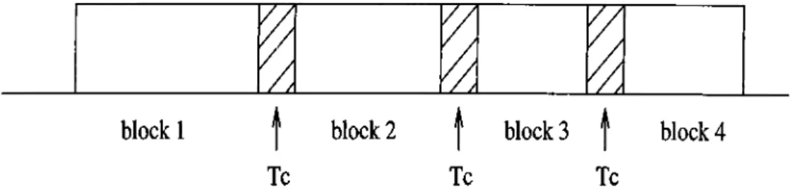
Figure 3.1: Representation of a schedule as blocks of jobs

If we consider the jobs sharing the same tool as a block, a schedule can be viewed as blocks of jobs separated by tool changes (see Figure 3.1). This representation would be helpful to gain more insight into the problem structure. Note that, the length of blocks do not have to be same. This is because, when we cannot assign more jobs to a tool although the tool life has not flnished, there is no meaning in waiting till the end of tool life to make the tool change. So, in such cases, the tool is immediately replaced by a new one, and the block length shows the used portion of the tool. This property of the tool change problem is another point that makes it different from the existing models. In models of scheduled maintenance (see [19], [20], [17], [18] for examples) the unused capacity of the machine is counted as wasted time which is added to the flowtime of the latter jobs. However for the tool change problem this is not the case.

With this representation, we can consider the blocks as job strings which must be processed together, and has length tj+ T c. Then we know the following

structural properties of the problem from the scheduling literature [6];

• If jobs q and r are within the same block, then

q precedes r if p, < ·

• Furthermore, for blocks i and j: i precedes j if ii±2!£ < £diZ£

Thus we conjecture that, in an optimal schedule, blocks should be in non­ increasing order of the number of jobs they have, and the jobs in a block must be in SPT order.

The total flowtime of such a sequence of jobs has two main parts, the first part shows the total flowtime without tool changes, and the second part is added as the increase in flowtime as a result of tool changes. When we ignore the tool changes, the total flowtime of a schedule cr is equal to:

CT = ¿ ( « - 9 + 1)P[9] 9=1

When we introduce the tool changes into the picture, we have to add the contribution of tool changes to the objective function, which can be written as:

c ’2 = E y - i)ri’ Tc

j=l

This follows from the fact that before each job using the jth tool, ( j — 1)

tool changes would have been done, and this would increase each such jo b ’s completion time by Tc.

Then total flow time of a schedule a is:

z , = Cl + Cl = ' £ ( n q + 1)P[„ + E y

-9=1 j = l

These two parts of the objective function are conflicting in terms of the requirements to be minimized. In order to minimize C f , we should apply SPT,

that is, the shorter jobs should be put in earlier blocks, and longer jobs be remained for the later blocks. In an SPT schedule, the number of jobs in the blocks, 7/j ’s are in non-increasing order of j , since we can assign less number

of jobs to a block if their processing times are long. And for some instances this may increase the number of tools used, under-utilizing the tool life in later blocks. On the other hand, for C2 to be minimized, the number of blocks

should be decreased, and this can be done only if some larger jobs are scheduled early so as to maintain balance in the later ones. From this aspect, problem is similar to bin-packing problem, but certainly not equivalent. Especially as

Tc gets larger, this conflict between cost components makes the problem more diiflcult to solve.

Having defined some basic properties of the problem, we can analyze it in more detail. In the following sections, the complexity issues, and the performance of SPT heuristic for this problem will be discussed.

3.2.1

Complexity of the Problem

Although flowtime problem is very easily solved optimally by the SPT rule, when there are tool changes the problem becomes NP-hard in the strong sense. The proof will be done by transforming the 3-partition problem, which is a well- known NP-hard problem [11], into our problem, scheduling with tool changes. So, first we should state the 3-partition problem:

Given 3m integers { ai, 0 2,· · · ,a3m } such that a, = mB and j <

ttq < Y , can this set be partitioned into m 3-tuples such that Y^aq = B for each 3-tuple?

The following theorem shows that tool change problem is NP-hard.

Theorem 3.1: 1/to o l change/X^Ct is strongly NP-hard.

an instance of (P) such that; n = 3m Pq = Ctq, let 0 1 ^ 0 2 · · · ^ 0 3^ Tl^ B n ^ ~ 9 + l)ön-g+l 9=1 Tc = C » A

It was shown that for any schedule cr,

AV

^<7 = C f + C2 = X ](n - 9 - l)i?JTc

9 j = i

Q u estion : Does there exist a schedule with total completion time, J2g- =lC'9 <

If 3-partition has a solution the answer is YES.

If 3-partition exists 3m(m — 1) = Then, J=i C*9 = 9 + 1)P[9] + E ( *

-g=i g=i i=l

- A . i\ 3m(m - 1 )^ - “ 9 + 1)P[9] H---2---^

< M i: ; - , i j g

Thus, the answer to question is yes.

If partition does not have a solution, the answer is NO.

If 3-partition does not exists, any schedule will have to use m + / (/ > 0) tools and for I < i < m -f- /, 0 < 7/j < 3 will be true.

Let A i = 3 — Tji for I < z < m. Then we know that Aj > 0 for at least one

i-i 1 < « < m . Moreover, rji = 3m. Thus

m m-\-l +

S

i

I

¿ = 1

^ Vm+i — _(*)

4=1

For any schedule consider the second part of the flowtime value:

m-\-l m m-\-l [ ¿ ( * - 1)77,·+ { i - l ) r j i ] C 2=1 2=1 2=m+l m m+/ = E ( * - 1)(3 - A,·) + £ (i - l)r]i]C 2=1 2=m+l m m I = [3 - 1) - - l)A i + X ](m + i - l)rj^+i]C 2 = 1 2 = 1 2 = 1 = [ 3m(m — 1) - £ ( * - l)A i + m + ¿ ( 7· - l)i;^+i]C7 2 = 1 2 = 1 2 = 1 3m (m —1) ^ , NA ^ ·,

--- r----

l)Ai +

4=1

m 2 = 1 2 = 1

‘\ m ( m — 11 '

--- T---C + [m ^ A* - ¿ ( 7 - l)A j + ¿ ( 7 - l)rj^j^i]C (using (*) )

2 = 1 2 = 1 2 = 1

3m(m — 1)

C + i + l)A i + — V)rjjn-\-i\C

4 = 1 2 = 1

Clearly, the term within the braces is > 1. Hence, for any schedule, C2 >

+ C. Thus,

¿ c , > 3"‘(’! - !)<? + c

Thus, the answer to question is NO. Hence it is shown that, even for the special case, the problem is reduced to another problem that is known to be strongly NP-hard, namely 3-partition problem. This proves the strong NP-Hardness of our problem. □

Furthermore, even when we fix the number of tools that can be used as a constant, the problem still remains NP-hard. This is shown by the following theorem.

Proof: Proof will be done by using a reduction from the partition problem. Partition problem is stated as follows:

Given a set y4 = can we partition A into subsets Ai, and A2

such that = T,ieA2 ?

This problem is well known to be NP-Hard [1 1].

Create an instance of our problem such that:

m = 2 (number of tools)

n = number of jobs Pq = <lq

1

T L = ^ T , a .

In this instance, it is obvious that there exists a feasible schedule if and only if partition problem has a solution. Therefore, answering the question if there is a feasible schedule with 2 tools is NP-Hard. Since even the feasibility check is NP-hard, the problem is NP-hard as well. □

Thus we have shown that tool change problem is NP-hard, even when the number of tools is fixed, and as low as 2.

3.2.2

Performance of SP T Heuristic

As mentioned before, for the classical flowtime problem, SPT is a very powerful rule. And, when T c 0, it is obvious that SPT would be optimal, since then

the problem would reduce to the classical 11| E C'i problem. However, for our problem, depending on the magnitude of T c value, it may not perform as well. We can illustrate this with an example:

Let n = 5, Tl = 6 , and Tc = 2. And let the pg values for 5 jobs given as 1,2,2, 3 ,4. The SPT schedule would be as follows with respect to the processing

times:

1 2 2 T c 3 T c 4

where T c represents a tool change at that point. So, SPT schedule requires 2

tool changes, and the total flowtime for this schedule equals 3 5.

On the other hand, the optimal schedule would be:

1 2 3 T c 2 4

with total flowtime equal to 34.

Now, let Tc = 0.5 for the same example. This time, Zs = 30.5, where flowtime of the second schedule (which was optimal for Tc = 2) becomes 31.

As the above example suggests, the performance of the SPT heuristic changes with different Tc values. Intuitively, for small values of Tc, SPT should perform well, whereas it may lose power as T c value increases. In order to understand if this intuition makes sense, we have made some experiments on small problem instances for which we can And the optimal objective function value. Different problems are solved for all possible cases with n = 8,12,16

and ^ = 0.1,1,10. For each of these 8 cases except n = 16, 4 problems with

K s = 3 and four having K s = 4 are solved by SPT and compared with the optimal result. For 16 jobs we were not able to find the optimal solution when

Ks = 4 in four hours of CPU time, so we have only considered K s = 3. The results are summarized in Table 3.1. For each combination of n and ^ values, the minimum percent deviation (MinPD), average percent deviation (APD) and maximum percent deviation (MaxPD) of the results obtained by SPT rule from the optimal objective function value are presented in this table.

As we can see from these results, performance of the SPT rule gets worse for our problem as tool change time increases. When the ^ value is small (as 0.1), SPT is optimal most of the time, especially for the small problem sizes SPT rule dominates. Intuitively, one thinks that as T c oo, the problem can be seen as a bin packing problem, so as to minimize the number of tool changes needed, since this time T c value would dominate. However, although

Tc/Tl = 0.1 Tc/Tl = 1 Tc/Tl= 10

n MinPD APD MaxPD MinPD APD MaxPD MinPD APD MaxPD

8 0.00 0.00 0.00 0.00 1.2869 6.2500 0.00 3.8193 16.1591

12 0.00 0.00 0.00 0.00 1.2374 4.3564 0.00 5.5632 17.0616

16 0.00 0.0444 0.1776 0.00 2.0224 4.5399 0.00 5.8903 11.9041

Table 3.1: Comparison of SPT performance with optimal values

this observation is logical, the optimal bin packing solution for tool change problem does not always give the optimal flowtime objective.

Moreover, when T c —> oo, the performance of SPT heuristic for our problem does not coincide with its performance for the bin packing problem. The worst instance that SPT rule can behave for the bin packing problem is given by Johnson et al. [15]. This example is presented below and the ratio of C2

values for optimal bin packing solution and SPT solution is calculated. Note that as T c —>· 0 0, C^·

Let Tl be 101 and T c —> 0 0. We have five job types with the following

processing times pi, and number of jobs Sk for job type k\

type A Pi - 51 = 1 0

type B Pi = 34 5B = 1 0

type C Pi - 16 S c = 3

type D Pi = 10 s d = 7

type E Pi = 6 s e = 7

The optimal bin packing solution will use 10 tools with the following allocation of jobs to tools:

Tools 1 - 7: (E D B A)

This sequence has the C2 value equal to 156Tc.

The SPT sequence will use 17 tools with the following allocation: Tool 1: {E E E E E E E D D D D D)

Tool 2: {D D C C C)

Tools 3 - 7 : (B B )

Tools 8 - 17: {A)

This sequence has C2 value equal to 160Tc.

As we see in this example even if the bin packing solution of the SPT rule has a performance ratio of = 1.7, its performance for our problem approaches

to = 1-025.

Furthermore, we can provide an instance where SPT schedule is better than the optimal bin packing solution, even when Tc approaches to infinity. Consider the following example:

Consider an instance where T c —> 0 0, Tl = 1, and there are four job types with the following processing times p,, and number of jobs Sk for job type k:

type A -> Pi = 1 + e type B ^ Pi = \ - e type C ^ Pi = \ - c = 6 SB = 2 Sc = 3 type D Pi = i - e sd = 4

The optimal bin packing solution uses 3 tools ordering the jobs as:

D D D D A A T c C C C A A T c B B A A

However, SPT rule would result in the following order:

D D D D C C C B B T c A A T c A A T c A A

with - l2Tc.

This shows an instance where SPT schedule can still be better than bin packing solution even if T c —> oo. Since there is no tool change before the first block, and SPT fills all the small jobs to the first block, the effect of tool changes on flow time of the jobs is reduced although it requires one more tool change to complete the jobs.

In the worst example we could find for the performance of SPT rule for

qS

our problem when T c ^ oo, the ratio was 1.5. This instance is illustrated below:

Let n = 6, Tl = 10 and processing times of jobs be given as 1, 2, 3, 5, 6, 6.

Then, if a job is represented by its processing time, the SPT sequence and the optimal sequence are as follows:

SPT: 1 2 3 Tc 5 Tc 6 Tc 6

Optimal: 2 3 5 Tc 1 6 Tc 6

The performance ratio of SPT would be = 1.5. This is the worst instance we have found for the performance of SPT rule when Tc approaches to infinity.

Having seen that SPT maintains its power for some instances, even when

Tc is too large for SPT to be optimum, it can be expected that there is a bound on the worst case performance of SPT heuristic. So, the question is, how bad can SPT behave in the worst case, even when Tc value approaches to infinity? It turns out that, the performance ratio of SPT is bounded above by a constant, which will be proved after stating some properties needed in the proof:

1. We stated before that, in an optimal schedule, blocks should be in non­

increasing order of the number of jobs they have, and within a block jobs are sorted in SPT order.

2. We know that the following relation holds between n and m:

^Pmin n > m >

Tl

where pmin is the minimum processing time value. Then i f n —^ o o = ^ m —»^oo also holds.

Having stated the necessary structural properties, we can investigate the worst case behavior of SPT heuristic.

In order to remind the notation and clarify the steps to be taken in the proof, let us rewrite the cost components and the expression for the performance ratio once more. We define the cost components as follows:

C'r = - 9 + 1)PM

q=l

CJ = E ( i - iW jT c

Then the total flowtime is:

z , = Cl + C l

Thus the performance ratio is:

Z s c f

+ E&,(< -

f> =

Zs-

c r + E f j : {i - lurVTo

c r

We are trying to prove that this ratio is bounded by a constant. First of all we have made an observation:

Assuming that SPT schedule is not the optimal one, it must use more tools than the optimal schedule. Because, SPT minimizes Ci, and if there were equal tools in S and S*, it would also minimize C2, since the //¡’s are non-increasing in i, and as i increases, the effect of rji on C2 also increases. Hence, if there

were equal number of tools in S and S*, S would be optimal.

So, based on the above observation, we can say that the part of for

i < Ks· is less than C f , i.e. if we define,

Cf =

+ A

Then C < Cf* . This means, we can write Cf* = 0(7, where 0 > 1

Consequently, the performance ratio would be as follows:

. ,

c !

1 , vf<s>+i + « - 1) ^ ^ , Vks*+i i — 1) - O'^

^ 0 +

EF=i{Ks*+i-l)

04>zl\'{i - 1 )

2DKs· + D ^ - D

We can find a bound on D using the bounds for bin packing problem. When we make the SPT order, the bin-packing aspect of the problem, which determines the number of tools used, is solved by NFI (next fit increasing) method. This means, starting with item 1 place it in bin 1. When packing item ji, put it in the highest indexed nonempty bin if possible, otherwise, place it in a new bin. The items are packed in the order of increasing sizes. SPT order exactly applies this method, when allocating tools to jobs. So, we can use the absolute bound for NFI (= 1.75) given by Anily et al. [3] in order to find a bound for Ks- Actually, the optimal schedule may not minimize number of tools, the optimal result of bin packing problem is a lower bound for Ks*·

So, we can say;

Ks

Ks* < 1.75

then

D = K s - Ks* < 0.75Ks*

So, putting (0.75.A'5·) instead of D in the last line of the previous equations, we get.

C ! ^ 1 2.0625/^1. - 0.7 5/1:5.

c f

where ^ > 1, and (¡>>1.

seems that when Ks* = 2, p < 4.375. As Ks* increases this value decreases, and when Ks* oo, p < 3.0625. Hence, we conclude that the performance ratio for SPT is absolutely less than 4.375.

3.2.3

Conditions for optimality of SPT

As mentioned before, it is obvious that when T c = 0, the SPT rule gives an

optimal sequence. We searched for other conditions which guarantee optimality of SPT schedule even when T c —»· oo. Among them some are trivial such as:

In this case, any non-SPT schedule would be worse than SPT schedule since the number of tools used cannot be decreased. If p, > only one job can be assigned to a tool. If there are more than one jobs such that pq = 'LL·^3p'p schedule would assign them to one tool, whereas a

non-SPT schedule may miss this opportunity. Hence, we conclude that in this case SPT rule gives the optimal schedule independent of T c value. • K s < 2

In this case, Ks· < 2 must also hold. Because, SPT sequence already has the maximum number of jobs in the first block (hence minimum in the second block, which contribute to C^), and if 2 tools are enough, there

will be no decrease in by using one more tool in order to allocate at least as many jobs as . Since we know that SPT also minimizes we conclude that SPT schedule is optimum in this case.

In addition to these, we can find a bound on T c below for which the SPT rule gives an optimal sequence.

To find a maximum T c value below for which the SPT schedule will be optimal, we have considered an approach of comparing the cost components of the SPT schedule with any other non-SPT schedule. Here the absolute bound for worst case performance of SPT, found as 4.375, is used which is the

only absolute bound we have. We did not use the asymptotic value of 3.0625, because the value obtained at the end of these computations is asymptotically going to zero.

To find a. Tc value, a;, below for which SPT is optimal may have two meanings:

1) if T c < a; = > SPT is optimum 2) if SPT is optimum Tc < x

What we are looking for is the first one. So, we must find a minimum value for the right hand side of the equation (1) (whereas a maximum value would

be needed for the second part). Below is the calculations for the first part. Factoring out the Tc value from C2, we redefine the cost components with

a slight modification as follows:

Cl = - 9 + 1)P[,:9]

Then total flow time is:

CJ = E (i -

l)-vt

i=l

Z = Y^C^ = Ci + C2.Tc

Assume that there exists a schedule other than SPT schedule, which gives the optimal objective value. In this case, for SPT schedule to be optimal the following must hold:

S is optimal C f + C^Tc < C f + C f T c

[ c ! - c f ) T c <

cf

T c <

c f -

c f

C f - C f ^ 4.375(Cf* - C f ) ^9 ^9 > 3.375C2^ 4.375A'„i„ > 3.375E & ( i - 1) ., ? 4 .3 7 5 A L .

3.375E&,(!-l).>)i

4.375AL„

3.376i,f/lfs(/is - l)/2

2

(3)

where A ^j„=m inim um difference in processing times of given jobs (greater than zero).

While writing Equation (2) we tried to find the minimum possible deviation of the total flow time of a non-SPT schedule from an SPT schedule. If only the two adjacent jobs with minimum difference in processing times (not equal to zero) are interchanged, the minimum deviation would occur. It can be calculated as:

(n - /)pJ+ij + { n - l - l)pg - [(n- l)pfi^ + (n- / - l)p^+i]] = pf+q - p| =

where / shows the rank of the jobs with minimum difference in processing times. Then, from (1) and (3) we can say that if

2

.

AL,:„

T c <_{- „.s}

rjUKl - Ks)

then SPT schedule is optimum.

3.3

Summary

In this chapter, after giving the definition of our problem together with the underlying assumptions, the characteristics of the problem has been analyzed.