Maintenance and marginal cost analysis of a two-unit cold standby system

(1)

A T H E S I S

S U B M I T T E D T O T H E D E P A R T M E N T OP IN D y S T R lA L

E N G IN E E R IN G

A N D T H E I N S T I T U T E OP E N G IN E E R IN G A N D S C IE N C E S

O F B IL K E N T U N I V E R S I T Y

IN P A R T IA L F U L F I L L M E N T O F T H E R E Q U IR E M E N T S

FO R T H E D E G R E E O F

M A S T E R O F S C IE N C E

C h o k ri H a m d a o u i

A u g u s t, 1997

(2)

A THESIS

SUBMITTED TO THE DEPARTMENT OF INDUSTRIAL ENGINEERING

AND THE INSTITUTE OF ENGINEERING AND SCIENCES OF BILKENT UNIVERSITY

IN PARTIAL FULFILLMENT OF THE REQUIREMENTS FOR THE DEGREE OF

MASTER OF SCIENCE

By

. , V - C.. C, .■

/

Chokri Hamdaoui

August, 1997

(3)

} Q - £i

(4)

I certify that I have read this thesis and that in my opinion it is fully adequate, in scope and in quality, as a thesis for the degree of Master of Science.

Assoc. Pro; (Principal Advisor)

Assist. Prof. Selim Aktiirk

/\ y-« 4· I 3 ^

Assist. Prof. Emre Berk

Approved for the Institute of Engineering and Sciences:

Prof. M ehm et^^ray

(5)

M A IN TE N A N C E AND M ARGINAL COST ANALYSIS OF A

T W O -U N IT COLD STAND BY SYSTEM

Chokri Hamdaoui

M.S. in Industrial Engineering

Supervisor: Assoc. Prof. Ülkü Gürler

August, 1997

The Marginal Cost Analysis (M CA) of maintenance policies is a concept gaining interest in the recent years. This approach, due to Berg, has been categorized as an Economics Oriented Approach, as different from the classical probability centered approach. The MCA has been successfully applied to the Age Replacement and the Block Replacement policies, and was shown to be flexible enough to permit extensions and generalizations.

In this thesis, we apply the MCA approach to a more complex model. We consider a two-unit cold standby system. Upon failure of the working unit in the time interval [

0

,T) the unit is replaced by the standby unit if available. If the standby unit is in repair, the system is down, and a downtime cost is incurred. The item inspected at time T is in one of two states: “good” , or “critical” . The good unit continues operation, whereas a unit in critical state is sent to repair. The switchover is immediate. We derive and compare the marginal cost function as well as the long-run cost per unit time function.

K ey words: Maintenance Policies, Age Replacement, Block Replacement,

Cold Standby System, Marginal Cost Approach.

(6)

SOĞUK YEDEKLİ İKİ BİRİMLİ BİR SİSTEMİN

B A K IM /O N A R IM V E MARJİNAL M A L İY E T ANALİZİ

Chokri Hamdaoui

Endüstri Mühendisliği Bölümü Yüksek Lisans

Tez Yöneticisi: Doç. Ülkü Gürler

Ağustos, 1997

Bakım/onarım politikalarının Marjinal Maliyet Analizi (M M A) ilgi kazan makta olan bir kavramdır. Berg tarafından ortaya atılan ve klasik olasılık yaklaşımından farklı olan bu kavram Ekonomik Bakışaçılı bir yaklaşımdır. MM A yaklaşımı yaşa bağlı ve blok yenileme politikalarında başarlı olarak uygu lanmış ve çeşitli yönlerde genelleştirilecek kadar esnek olduğu gösterilmiştir.

Bu tezde M M A daha komplike olan iki-birimli yedekli sistemlere uygu lanmıştır. Çalışan birim [

0

,T) aralığında bozulduğunda eğer yedek birim hazır durumdaysa onunla değiştirilmektedir. Eğer yedek birim tamirde ise, sistem durmakta ve bir durma maliyeti ortaya çıkmaktadır. T zamanında kontrol edilen birim “iyi” ya da “kritik” durumda olabilmektedir, “ iyi” durumda olan makina çalışmaya devam etmekte, “kritik” ise tamire gitmektedir. Makina değişimi anında olmaktadır. Bu çalışmada ortalama maliyet ve marjinal maliyet fonksiyonları bulunmakta ve karşılaştırılmaktadır.

Anahtar sözcükler: Bakım/onarım Politikaları, Yaşa Bağlı Yenileme, Blok

Yenileme, Soğuk Yedekli Sistemler, Marjinal Maliyet Analizi.

(7)

(8)

I am mostly grateful to Dr. Ülkü Gürler, who has been supervising me with patience and interest, for suggesting this interesting research topic, and for being helpful in any way during my graduate studies.

I would like to extend my thanks and gratitude to Dr. Selim Aktürk and Dr. Emre Berk for showing keen interest in this research area and for kindly accepting to read and comment on this thesis.

Finally, special thanks are due to all my instructors, friends, and colleagues, who helped and supported me throughout my studies.

(9)

1 INTRODUCTION

1

1.1 RELIABILITY AND DESIGN FOR R E L IA B IL IT Y ...

1

1.2

INTEGRATING MAINTENANCE A C T IV IT Y INTO PMS . .

2

1.3 PERFORM ANCE MEASURES AND RELATED CONCEPTS

2

1.3.1 What Causes Failure?

4

1.3.2 Preventive M a in te n a n c e ... 4

1.3.3 Performance M e a s u r e s ... 5

1.4 P R E L IM IN A R IE S ...

6

1.5 SCOPE OF THE T H E S I S ... 9

2 LITERATURE REVIEW

10 3 THE MODEL AND POLICIES

25

3.1 THE MODEL D E S C R I P T I O N ... 25

3.2 THE M ARGINAL COST APPROACH AND ITS M OTIVATION 26 3.3 POLICY 1 ... 28

(10)

3.3.1 Cycle L e n g t h ... 29 3.3.2 Cycle C o s t ... 30 3.4 POLICY

2

... 31 3.4.1 Cycle L e n g t h ... 31 3.4.2 Cycle C o s t ...

33

3.5 POLICY COMPARISON

35

3.6 M ARGINAL C O S T S ... 35 3.6.1 Policyl ... 35 3.6.2 P o lic y 2 ... 37 3.7 E X P E R IM E N T A T IO N ... 39 3.7.1 Policy 1 ... 40 3.7.2 Policy 2 ... 40

4 GENERAL MODEL

48

4.1 GENERAL M O D E L ... 48

4.1.1 Cycle Length - Without I n s p e c t io n ... 49

4.1.2 Cycle Length - With In s p e c tio n ... 51

4.2

L I M I T S ... 64

4.2.1 As p ^

0

64 4.2.2 As p

1

65 4.3 THE M ARGINAL C O S T S ...

66

(11)

4.3.1 Generalized Policy

1

4.3.2 Generalized Policy

2

66

68 4.4 ASY M PTO T IC B E H A V IO R ... 76

4.5 SPECIAL CASE: EXPONENTIAL LIFETIMES 77

5 NUMERICAL RESULTS

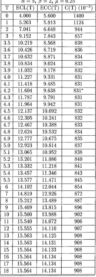
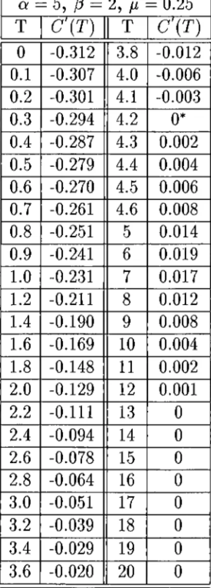
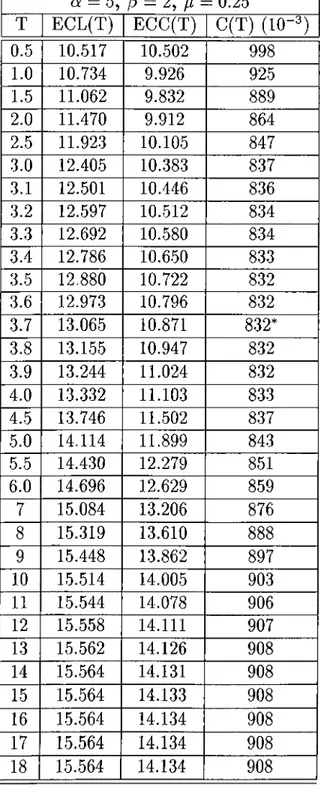
5.1 MODEL PARAM ETERS

5.2

p CONSTANT 5.3 p A FUNCTION OF r

82

82 83 89

6 CONCLUSION

95

(12)

3.1 Sketch of the S y s t e m ... 26

3.2

A Typical Realization of the Processes Z(t) and R ( t ) ... 27

3.3 Total costs C (T ), and marginal cost, t/(T ), functions versus time

T. 29

3.4 Cycle length, for Policy

1

, with preventive maintenance carried out at intervals of length T: (a) X < m in {T ,Y }·, (h) T < X <

Y; (c) T < Y < X ] (d) Y < T < X·, (e) Y < X < T. 44 3.5 Cycle length, for Policy 2, with preventive maintenance carried

out at intervals of length T: (a) X < m m {T , F } ; (b) T < A” < F ; (c) T < F < AT; (d) F < r < X ; (e) F < X < T. 45

3.6 Cost curves, C {T ): Comparison of Policy

1

(P I) and Policy

2

( P 2 ) ... 46

3.7 Cost curve, C'(T), and marginal cost function, r /(r ), versus replacement age T , for the simple Policy 1 ... 46

3.8 Cost curve, C {T ), and marginal cost function, rj{T)^ versus replacement age T, for the simple Policy 2 ... 47

(13)

4.2 Cycle length: (a) The process Z(t) enters state 0 directly from state

1

. (b) The process Z(t) visits state

2

before state 0... 50

4.3 Cycle length, generalized policy

1

, with inspection carried out at intervals of length T: (a,) X < m in {T ,Y }] (b) T < X < Y ;

{ c ) T < Y < X ; i d ) Y < T < X - , { e ) Y < X < T ... 80 4.4 A typical realization of the system, for generalized Policy

2

. . . 81

5.1 Cost curve, C '(T), versus inspection interval T , for the degenerate case p = I ...

88

5.2

Cost curve, C {T ), and marginal cost function, versus

inspection interval T, with p = 0 . 5 0 ...

88

5.3 Cost curve, C'(T), and marginal cost function, p {T ), versus inspection interval T , with p = 0 ... 89

5.4 Cost curve, C'(T), and marginal cost function, p (T ), versus inspection interval T , with S = 0 . 9 5 ... 94

5.5 Cost curve, C'(T), and marginal cost function, p ( r ) , versus inspection interval T, with 6 = 0 . 5 0 ... 94

(14)

3.1 Numerical Results, Policy

1

41

3.2

Numerical Results, Policy

1

: Cost R a t e s ... 42

3.3 Numerical Results, Policy 2 ... 43

4.1 Analytical Results for Exponential Lifetime and repair Distri butions ... 77

5.1 Numerical results. Generalized Policy

1

, for the degenerate case

p - 1 ... 84

5.2

Numerical results, generalized Policy

1

, with p = 0.50 85 5.3 Numerical results, generalized Policy

1

, for the special case p = 0

86

5.4 Marginal Cost Values for Various Values of p ... 87

5.5 Numerical results, generalized Policy

1

, with 8 = 0 . 9 5 ... 91

5.6 Numerical results, generalized Policy

1

, with 8 = 0 . 5 0 ... 92

5.7 Marginal Cost Values for Various Values of ... 93

(15)

IN T R O D U C T IO N

1.1 RELIABILITY AND DESIGN FOR RE

LIABILITY

The field of reliability analysis dates back to the second world war. It was an outcome of problems with electronic systems designed during the 1940’s. The growth in complexity of the electronic systems prompted the US Air Force, Navy and Army to establish committees to investigate the reliability problem. In 1952, the Department of Defense established the Advisory Group on Reliability of Electronic Equipment (AGREE). In the recent years, the field of reliability has become important for systems design and development.

Reliability must be considered early in the design process of a system, where changes can be most easily and economically done. During this design process, the system configuration is chosen. Evidently, the choice of the system configuration has a direct effect on the reliability level. During the design phase, a preliminary reliability analysis should be performed, in addition to the other design factors. The system designer should be familiar with the basic reliability analysis concepts that can be used as performance measures to evaluate the system. It is important that the designer evaluate the reliability

(16)

levels, costs and trade-olFs to come up with a final decision or choice.

1.2 INTEGRATING MAINTENANCE AC

TIVITY INTO PMS

Maintenance planning should be integrated in the Production Management System (PM S). In any organization, there are many resources such as workforce, equipment, machinery, work in process, raw materials, etc. However from a management viewpoint, the primary and most valuable resources are time and information. More specifically, timely information is of paramount significance, and is the key to success of today’s factory. The reason is obvious. For example, late deliveries of product may cause loss of customers’ good will. A plant may have the capacity to produce, but may not have the capacity to produce so many units in a certain period of time. Of course, the issue raised here is Production Activity Control (РАС), and its interface with PMS. We believe that reliability considerations should be integrated in РАС. Such considerations influence РАС in carrying out functions such as operation scheduling and loading, manufacturing order approval and release, capacity and quality control, process evaluation with respect to material and equipment costs and availability.

1.3 PERFORMANCE MEASURES AND RE

LATED CONCEPTS

The concept of a system is needful.

D e fin itio n

1

A system is a collection o f entities (e.g. people, machines, etc.)

(17)

A system is completely characterized by its state vector, a collection of

variables that contain all the information necessary to describe the system.

Grant & Leavenworth [29] suggest the following definitions for reliability.

Reliability is the probability of a device performing its purpose adequately for the period of time intended under the operating conditions encountered.

The reliability (of a system, device, etc.) is the probability that it will give satisfactory performance for a specified period of time under specified operating conditions.

The following definitions are suggested by AGREE.

Failure; the inability of an equipment to perform its required function.

Reliability: the probability of no failure throughout a prescribed operating period.

Similar definitions are due to Smith [54].

Failure: non conformance to some defined performance criterion.

Quality: conformance to specifications.

Reliability is the extension of quality into the time domain, and may be rephrased: the probability of no failure in a given period. Alternatively, quality is the projection of availability onto the space where time is zero.

These definitions are similar. However, there is no consensus as to what constitutes ‘ satisfactory performance.’ Naturally, this depends on the use as well as on the operating (or environmental) conditions. For example, a particular chip might have a short life under one set of specifications, and a long life under another set of specifications.

For repairable systems, the concept of minimal repair was first introduced to the literature by Barlow and Hunter [5]. Upon minimal repair, the repair

(18)

action returns the system into an operational state in such a way that the system characteristics are the same as they were just before failure, i.e. the system is as good as old. In other terms, the repair restores operability, but makes no improvement. Mathematically, that means that the hazard function following a (minimal) repair is undisturbed, so that the failure process in the process is independent of this and of any other past repair action.

1.3.1 W h at Causes Failure?

There are many causes of failure, known as stresses. Smith [54] classifies stresses into two categories:

a) Environmental: — Temperature, — Radiation

— Shock (mechanical, thermal) — Vibration

— Humidity

— Ingress of foreign body. b) Self-generated:

— Power dissipation

— Applied voltage and current — Self-generated vibration — Wear

1.3.2 Preventive Maintenance

These are systems in which the operating units are sent for preventive maintenance according to an age-specific probability distribution. When the

(19)

age of an operating unit is in the interval { x , x + A ), it is sent for preventive maintenance with probability o(a;).A, provided that this action of scheduling the preventive maintenance of the unit does not result in a system failure. Otherwise, the preventive maintenance is either deferred until one of the units under repair becomes available, or the preventive maintenance is cancelled. The concept of preventive maintenance is useful only when the failure rate of a unit is an increasing function of age, x, and the expected duration of maintenance is not larger than that of the repair time duration.

1.3.3 Performance Measures

We present some of the performance measures found in the literature of interest from the system’s design and analysis viewpoint.

One of the performance measures is termed serviceability, defined as the ease with which a system can be repaired. Clearly, ease of serviceability should be planned at the design stage, as it is a characteristic of the system’s design. However, this is not easy to measure on a numerical scale. Usually, it is measured by ranking, or by specifically developed rating procedures.

Maintainability is another performance measure, defined as the probability

that a failed system can be made operable in a specified interval of downtime, which includes the total time that the system is out of service. Downtime comprises failure detection time, repair time, administration time and the logistics time connected with the repair cycle. The maintainability density function describes probabilistically how long a system remains in a failed state (or down).

A more restricted performance measure is termed repairability.

Repairability is the probability that a failed system will be restored to a

satisfactory operating condition in a specified interval of active repair time. This performance measure helps quantify the workload of the repair facility, hence it allows a managerial support.

(20)

Operational readiness is the probability that either a system is operating or

can operate satisfactorily when the system is used under stated conditions.

Availability is the probability that a system is operating satisfactorily at

any point in time. It considers only operating time and downtime, thus it excludes idle time. Availability is a measure of the ratio of the operating time of the system to the operating time plus the downtime. Therefore, it includes both reliability and maintainability.

Intrinsic availability refers to the probability that a system is operating in

a satisfactory manner at any point in time when used under stated conditions. Hence, time is confined solely to operating and active repair time. Availability is always smaller than or equal to the intrinsic availability. The difference between these two performance measures can be viewed as a measure of administrative and logistics time related to the repair cycle.

1.4 PRELIMINARIES

D e fin itio n

2

Lifetime o f a component is the time, usually random, from the

beginning o f the operation until the occurrence o f a failure.

The reliability, or survival probability, is formally defined.

D e fin itio n 3 The reliability o f a component, with lifetime X having a

distribution F { · ), is F { x ) =

1

— F { x ) .

D e fin itio n 4 The conditional reliability o f a component at age t is the

probability the component will survive x more time units given that it is operating at age t. Formally, F {x \ t) = if F{ t ) > 0.

D e fin itio n 5 The failure rate r{t) at time t, o f the random variable X is,

r(t) = M

(21)

where F{ t ) ^ 0, and the density f { t ) exists.

A primary role is played by the failure rate function, sometimes called the hazard rate, force of mortality, and intensity rate. Failure rate of a component at time t is proportional to the probability that it will fail in the next short interval given that it is operational at the start of that time interval.

The failure rate has a particular usefulness in reliability analysis. The probability that a component will fail in the next A time units (for infinitesimal A ) given that the component is surviving now is equal to r{ t ) A. If r{t) is an increasing function of t, then the lifetime distribution F{ t ) is an Increasing Failure Rate (IFR) distribution. This describes a class of distributions corresponding to adverse aging. Note that IFR class can alternatively be characterized by decreasing conditional reliability, F { x | i), as a function of t, for each a; >

0

. If r{t) is a decreasing function of t, then the lifetime distribution F{ t ) is a Decreasing Failure Rate (DFR) distribution. In this case, aging is beneficial. A component whose lifetime distribution is in the DFR class has increasing survival probability, or equivalently, it has increasing conditional reliability, F { x | f), as a function of f, for each a; > 0. The failure rate function r{t) at age t is derived from the conditional reliability at age t,

r(t) =

lim i [ l

-

F(A I i)l

A - o A F{ t ) ‘ = ,im A-^oA F{ t ) F( i ) m

F{ty

1

j ^ + A ) A

Some useful identities are straightforwardly obtained from the above definitions. The reliability function and the failure rate function are intimately related to each other. Multiplying equation (

1

) by —

1

, then exponentiating.

(22)

we have

- r { t ) m

F{ty

(2)

Upon integrating both sides of equation (

2

) with respect to i,

— / r{t)dt — \ogF{x)

J 0

F{ x ) =

D e fin itio n

6

The hazard function is the cumulative failure rate up to age x.

Formally, it is

R( x) —

f

r{t)dt (3)

J O

The reliability function and the hazard function are related to each other, as follows,

F { x ) ^

₍₄₎

D e fin itio n 7 Age Replacement Policy (A R P ) is a policy where the component

is replaced upon failure or at age T, whichever comes first. If ci is the replacement cost at failure and c^, (t) < C

2

< c\), is the replacement cost

at age T , then the average long-run cost per unit time is given by,

CiF(T) + C2F{T)

C( T) =

¡0 m u

(5)

D e fin itio n

8

Block Replacement Policy (BRP) is a policy where the compo

nent is replaced upon failure and at times T, 2T, 3 T ,__ The expected cost per unit time, in the long run, is given by,

Cim(T) + C

2

C ( r ) = ₍₆₎

where m{ T) is the renewal function o f failures, that is the expected number of failures in the interval [

0

, T ).

(23)

D e fin itio n 9 The Failure Replacement Policy (FRP) is a policy where no

preventive replacements are made at all. FR P is a non-preventive policy, where action (replacement) is taken only after the failure has occurred.

Under FRP, the long-run average maintenance cost per component per unit time is where c is the replacement cost, and r is the expected life of a component. The result follows from the renewal theory. The interested reader is referred to Barlow & Proschan [7].

1.5 SCOPE OF THE THESIS

In this thesis, we study and perform Marginal Cost Analysis of a two-unit cold redundant standby system, supported by one repair facility. Our objective is to determine the optimal preventive maintenance time that minimizes the expected cost per unit time in the long run.

In Chapter

2

, we review the related literature. Chapter 3 provides a complete description of the model. Two maintenance policies are studied. Their Marginal Cost Functions are derived. In Chapter 4, we present a general maintenance model and derive its objective and Marginal Cost Functions. Numerical results for this model are provided in Chapter 5. Finally, in Chapter

(24)

LITE R A TU R E R E V IE W

The earlier work on reliability theory and replacement problems is the book, Barlow & Proschan [

6

]. The subsequent version of this book, Barlow & Proschan [7], is a good reference. It treats a wide range of topics, including coherent structure theory, the theory of extreme value distributions, fault tree analysis, availability theory, shock models, the Marshall-Olkin multivariate exponential distribution, as well as dependence of various kinds among random variables. This book is intended for reliability analysts, operations researchers, and statisticians.

Many survey papers covering the literature in maintenance and reliability theory have been published, including McCall [41], Pierskella & Voelker, Sherif & Smith [52], El-Neweihi & Proschan [

21

], Valdez-Flores & Feldman [57] and Cho & Parlai’ [17]. Review papers of standby systems include Osaki & Nakagawa [45], Kumar & Agarwal [38], and Yearout et al. [60]. Abouammoh & Quamber [

1

] trace the development and application of the statistical theory in modeling and solving problems in reliability engineering. They review criteria of aging; partial ordering; closure properties; discrete aging and shock model; and testing of exponentiality versus aging.

We start by single unit maintenance systems and policies, then we review some multi-unit systems. Finally, we review the two-unit redundant standby

(25)

systems.

Berg & Epstein [12] describe and compare three failure replacement policies: the age replacement policy; the block replacement policy; and the failure replacement policy. They propose a rule to choose the best (least costly) policy under some conditions specified on model parameters. Langberg [40] studies and compares age replacement policy (A R P ) and block replacement policy (B R P ), based on number of failures and removals. The number of renewals in the time interval [

0

, s] under ARP is shown to be stochastically smaller than the number of renewals in the same interval under the corresponding BRP. The author introduces the concepts New Better Than Used (NBU) in sequence and New Worse Than Used (NW U) in sequence. Under the assumption of NBU in sequence, the author shows that the number of failures in [0, s] under ARP is stochastically smaller than the number of failures in [

0

, s] when no replacement is applied.

The age replacement policy is studied by Berg [9]. Using renewal theory, and continuous Markov decision processes, he proves that it is an optimal decision rule amongst all reasonable replacement policies. Block et al. [15] propose a general age replacement model with minimal repair. It is assumed that the cost of a minimal repair is dependent on the number of minimal repairs done so far. Two kinds of replacement are considered: planned (at age T ) and unplanned replacement (upon failure, with probability p(y), where y is the age). They also consider a shock model, where the system is replaced at a fixed cost at periods T, 2T, 3T, etc. The authors derive the total expected long-run cost per unit time, and provide optimal results (replacement age,

T*) for finite and infinite horizon. A similar study is done by Block et al.

[14]. They investigate a maintenance policy where upon failure a maintenance action is undertaken. However, the maintenance action is a complete repair with probability p{t), and is a minimal repair with probability q{t) =

1

- p{t), where t is the age at failure. Repairs are assumed to take negligible time. The authors establish that the successive complete repairs are a renewal process, and derive its interarrival distribution.

(26)

Another variation of the age replacement model is the paper by Tilquin & Cleroux [56]. They investigate periodic replacement policies with minimal repair and discrete adjustment costs. The adjustment costs are those costs incurred to keep the system operating. They suggest the replacement age that minimizes the expected maintenance cost per unit time over an infinite horizon.

Kamien & Schwartz [3.3] study the problem of optimal maintenance policy for a machine subject to failure. It is assumed that the natural probability of machine failure is increasing with age, whereas the value of the machine’s output is independent of age. There is the option of selling the machine at any time, at a salvage value decreasing with time. The authors use optimal control theory, and distinguish between the machine’s natural failure rate and actual failure rate resulting from the application of a preventive maintenance policy, including when to sell the machine.

Cleroux et al. [18] treat the age replacement problem with minimal repair and random repair costs. They assume instant repair and replacement. At failure, the unit is replaced or repaired depending on the random cost of repair. Under this policy, at failure, the equipment is replaced if the repair cost is greater than ¿ci, where ci is the replacement cost and ^ is a predetermined fraction (parameter). They provide a method to determine the optimal replacement age that minimizes the long-run expected total maintenance cost per unit time.

Barlow & Hunter [5] define and investigate two preventive maintenance policies, one applicable to simple equipment and one applicable to large, complex systems. Policy I performs preventive maintenance after to hours of continuous operation. Policy II performs preventive maintenance on the system when its total number of working hours reaches U, even if operation has been interrupted because of failure. Failures are assumed to be repaired minimally. The system is assumed to restore its as good as new state after a preventive maintenance. The optimum policy is the policy which maximizes the fraction of up-time, over long time intervals. The policies are compared under various restrictions on Tg, Tg, and Tm, defined as the expected time

(27)

to perform emergency maintenance, the expected time to perform scheduled maintenance, and the expected time to perform minimal repair, respectively.

A maintenance policy accounting for the accumulated damage is studied by Zuckerman [62]. It is assumed that upon failure, a system is replaced by a new identical one, and that the replacement cycles are repeated indefinitely. The system is subject to shocks occurring in a Poisson stream. The author establishes an optimal control limit policy, a policy in which the system is replaced either upon failure, or when the accumulated damage first exceeds a critical control level i^*. He provides the optimal replacement policy that maximizes the total long-run average net income per unit time, and the policy that maximizes the total long-run expected discounted net income.

Most maintenance and replacement models consider deterministic time horizon. Banerjee &: Kabadi [4] study optimal replacement policies under random horizon. Upon failure of a functional part, the part is replaced immediately to keep the system in operation. There is the option to replace the part by two brands having different unit costs and life distributions. The authors determine a time-dependent replacement policy that minimizes the expected operational cost. They establish conditions that secure the existence of the optimal policy.

Technological advances and learning effects have also been considered in modeling some maintenance and replacement problems. Goldstein et al. [26] analyze a machine replacement model with an expected technological breakthrough. They assume a stationary environment of the time at which a new technology may appear, and devise a dynamic programming method to determine the optimal replacement age of an operating machine that minimizes the expected cost in the long run. Chand et al. [16] investigate the single machine replacement problem with learning. They assume that there is a setup cost to replace a machine, and that due to learning this cost is a nonincreasing function of the number of setups made so far. They develop a forward dynamic programming algorithm to determine how frequently replacements should be done over a finite horizon. They also obtain optimal results for what is

(28)

effectively infinite-horizon problem, while only using data over a finite period of time. Nakagawa [43] study the effect of imperfect preventive maintenance. After repair, the unit is as good as new (i.e. repair is perfect). Preventive maintenance (PM ) is imperfect is the sense that with probability p after PM the unit is the same as just before PM, and with probability p =

1

- p it is as good as new. Repair and PM are assumed to take negligible time. The author studies three models: Model I the unit is repaired upon failure; Model II the unit undergoes minimal repair at failure; and Model III the failed unit is detected only by perfect PM. Expected cost rate is derived for each model, and is minimized and the optimal policy is determined.

After reviewing some well known maintenance policies, let us now focus on multi-state maintenance systems, with many units. Lam & Yeh [39] study optimal replacement policies of multistate deteriorating systems. They classify the deterioration of a system into a finite number of states (n

4

-

2

), and characterize it by a semi-Markov process. Furthermore, the failure rate function of the sojourn time distribution in each state is assumed to be independent of time. It is assumed that the system can be replaced at any point of time. Cost parameters, replacement and sojourn time distributions are state dependent. The authors investigate optimal state-age-dependent replacement policies that minimize the expected long-run cost rate. They show that under some regularity conditions the optimal policies have monotonic properties.

Kander [34] investigates inspection policies for deteriorating equipment. He deals with systems in which A^ +

1

quality levels can be diagnosed, characterizing them by a semi-markov process. He assumes no aging during the sojourn in any state. He develops optimal inspection policies yielding minimal loss. The optimal policy is a sequence of checking (inspection) times minimizing the loss per life cycle. He also deals with models of pure checking, truncated checking, and checking followed by monitoring.

Sharma et al. [51] study the transient behavior of multiple-unit reliability systems, characterizing a system by a Markovian process, representing the number of operable units at any point in time. They model the problem as a

(29)

birth and death process. The repair time and lifetime distributions of a unit are assumed to be exponential. For the system to be operable, there must be at least k ( k < n ) operable units. The authors derive the reliability and the availability functions of the system for the transient state.

Wilken L· Langford [59] study n identical systems assumed to operate independently, each characterized by an exponential time to failure with mean

1

/

7

. Upon failure of a system, it is immediately replaced by a spare (if there are any.) The authors start by writing the probability of exactly i failures in a time period of length t in the case where no spares are provisioned. Then, they establish a recurrence relation between this probability and the conditional probability of exactly i failures in time t, given that the first failure of any system is at time t'. Finally, by induction, they derive the expression for the probability of exactly i failures in a time period of length i, for the general case when s spares are provisioned.

Van Der Duyn Schouten & Vanneste [48] propose two control policies for a multicomponent system, consisting of M identical machines in series, with the objective of minimizing the long-run average cost of the system. Each component has four possible states: good (

0

), doubtful (

1

), bad (

2

), and down (3). The sojourn times in states 0 and

1

are taken to be exponentially distributed. The two policies are Policy A: a complete replacement is carried out if and only if a single component enters state

2

or

3

and the number of components in sate in state

1

is greater than or equal to K . Policy B: a complete system replacement is carried out at the first time epoch at which a component enters state 2 or 3 after the first moment at which the number of doubtful components has reached the level K . Average cost analysis of these policies is done, and the four states are identified with age intervals. Furthermore, the authors derive approximations for some performance measures, such as time to system replacement, and validate their results with simulation. Goel

al. [

22

] present a cost-benefit analysis of a complex system comprised of two subsystems A and B connected in series. Subsystem B has one unit whereas subsystem A has two identical units. Failure and repair times for each unit are exponentially distributed. Switchover is instantaneous. The system fails

(30)

either because of a failure of subsystem A or subsystem B, or because of a failure of subsystem B and one of the two units of subsystem A. The authors use the regenerative point technique, and derive some performance measures: mean time to system failure; availability measures; repairman busy period fraction. The authors perform profit analysis, and conclude that a high positive correlation between failure and repair times leads to a high mean time to system failure.

Drinkwater &: Hastings [20] study an economic replacement model of vehicles. They propose a theory of repair limits. They suggest two methods to determine the optimum repair limits, and show that these lead to financial savings. Dogrusoz and Karabakal [19] investigate a replacement problem of garbage collection trucks, with increasing operating costs and decreasing availability. Use the discounted value of all cash flows, they develop a measure, the average cost per unit quantity of service provided per truck load garbage collected throughout the service life of the equipment. They determine the optimal replacement age.

Baxter [

8

] derives some reliability measures for a two-state system. An alternating renewal process is used to model the operation and repair periods. The author defines an indicator variable Ik{t) which is equal to 1 if the system is operating at time t, and

0

otherwise, where A; =

0

if the system is initially down, and

1

otherwise. The concept of interval of a two-state system is defined as Rk{ x, t) = p{Ikiu) = IVu € [A,A + a;]} for A; = 0,1. The author introduces a new density function representing the density of the asymptotic recurrence time of a renewal process whose renewal is according to the distribution F , as ‘ip{·) = fii and

/^2

designate the expectations of F and G which are the distribution functions of the failure times and the repair times, respectively. Then the author establishes that the limiting interval reliability

R(^x) =

[1

— ^(a;)], where ^ is the distribution function with density ip. The author also derives expressions for the joint availability and for the forward recurrence times to break down at time t given that Ik{t) =

1

, A; =

0

,

1

.

(31)

asymptotic distribution for the time to system failure, for the

1

-out-of- (n +

1

) redundant cold standby system. There is one repair facility which starts repair only when the queue length becomes k. The repair time distribution is exponential, whereas the failure time distribution of the active unit is arbitrary. The author notes that in reality the time between failures of the active unit is considerably larger than the repair time. Using this observation, he shows that asymptotic distribution of the time to system failure is exponential. He takes the Laplace-Stieltjes transform of the system’s time to failure distribution, and shows that it converges to

(1

+ where s is the number of spare units.

Shao L· Lamberson [50] examine an n-unit cold standby system with built-in test equipment (B IT), which can detect system failure, distinguish and report failure mode and occurrence time, and record all the information to a data base. If the BIT cannot detect a failed active unit, a system failure occurs. BIT itself has a failure rate. Switching is instantaneous. Time to failure of a unit is exponentially distributed. Units are non identical. It is assumed that the switch is under the command of the BIT, and that the successful switching probability is k. By properly defining the states of the system, and treating it as a discrete-state, continuous-time homogeneous Markov process, the author establishes a set of first-order linear differential equations. These are solved by taking Laplace Transforms. The system reliability is obtained. A numerical example is considered for three identical units.

The two-unit cold standby systems have a particular importance. Osaki & Asakura [44] study a two-unit standby redundant system with repair and preventive maintenance. Using Laplace-Stieltjes transform (L.S.T.), the authors provide the distribution of time to the first system down, and derive the mean time. They assume arbitrary time distributions for failure, repair, inspection and preventive maintenance. Switchover times are instantaneous. After repair, the unit can operate perfectly. At age t, the operating unit is inspected. To avoid system downtime, an inspection is not performed when the other unit is not in standby. Failure time distribution of a functioning unit has IFR. They define four states, which are time instance of the system. Then they establish the distributions and their L.S.T. of the time between

(32)

these states. They provide an expression for the mean time to system down. In addition, they prove that repair is effective, under the condition that the failure rate of the failure time distribution is strictly increasing.

Gopalan & D ’Souza [27] investigate the two-unit system with a cold standby, with a single repair facility that performs repair and preventive maintenance, the lengths of which (i.e. service times) are governed by exponential distributions. Initially, one unit is in standby and one unit starts functioning. The times at which an operating unit is sent for preventive maintenance or repair are assumed to be exponential distributions. The authors derive the Laplace Transforms for the mean downtime of the system, and for the mean time to system failure, and obtain the availability and the reliability functions of the system.

Van Der Duyn Schouten & Wartenhorst [49] study a two-unit cold standby system with one repairman. After inspecting a failed unit, the repairman has the option to choose either a slow or a fast repair rate. The amount of work is known before repair is started. Additionally, the repairman can switch to the fast repair rate when the system breaks down. However, switching back to slow rate during a fast repair is not allowed. Based on the breakdown cost, the authors investigate long-run average costs. Using the theory of optimal control, and semi-Markov decision processes, they present some useful performance measures, including long-run average costs, all moments of system up- and downtimes, and system availability.

Wang [58] analyzes the steady state behavior of a cold standby system with

R repairmen. The repair follows the FIFO policy. At most M machines can

be operating simultaneously, while S machines are cold standby spares. Two failure modes are allowed, and they have equal probability of repair. Failure times and repair times are exponentially distributed. The failure rates depend on the failure mode: that is, there are two failure rates which are exponentially distributed. The author develops a profit model to determine the optimal number of standbys and the optimal number of repairmen simultaneously, constrained by system availability. He uses a direct search method, which

(33)

terminates after obtaining a global optimum value (S*,R*). The author uses birth and death balance equations, and describes the system by the number of failed machines in mode 1 and mode 2. A numerical illustration is provided. The profit function is unimodal, resulting in a unique optimal global solution. The author conjectures that the profit function is generally so, though not necessarily convex.

Gupta L· Chaudhary [30] study a two-unit standby system with Rayleigh downtime and Gamma failure time distributions. The system consists of two units: one priority and the other ordinary. The priority unit has three distinct failure modes: normal, partial failure, and total failure. The ordinary unit has 2 modes: normal and total failure. Allowed downtime is T^. System failure occurs if the repair of the priority unit is completed during the downtime which is assumed to have a Rayleigh distribution. The author identifies 6 states, depending on the state of each unit, and on whether in standby or repair. Using the technique of regenerative points, the author derives system characteristics, such as system reliability, transition probabilities, sojourn times, mean time to system failure, and the distribution of time to system recovery and its mean. Laplace and Laplace-Stieltjes transforms are used.

Agnihotri et al. [2] examine a two-unit cold standby system with 2 types of failure. The operating unit fails due to machinery defects as well as due to random shocks. The two units are non identical. Repair and unit life distributions are general. Failure rate of an operative unit after it undergoes the first shock is assumed to increase. The authors identify 8 up states and 2 down states. Using the regenerative point method, and Markov chains, the authors derive some characteristics of concern: transient and steady state transition probabilities; mean sojourn times in regenerative states; distribution of time to system failure; pointwise availability and steady state; availability of the system; expected busy period of the repairman and the expected number of visits he makes in the time interval (0 ,ij.

Gupta et al. [32] study a two-unit cold standby system, subject to random shocks and degradation. There is a single repairman. The two units are

(34)

one priority and the other ordinary. The priority unit gets preference over the ordinary unit for both operation and repair. The priority unit has three operative stages: excellent, good and satisfactory. Shocks occur randomly, and may only affect the priority unit. Only a unit in a failure mode is repaired. Shock time and repair time are exponentially distributed. After repair, a unit is as good as new. Using the regenerative point technique, the authors perform profit analysis, and derive measures of system effectiveness, such as: reliability of the system, and mean time to system failure; the expected up time due to each unit and the expected number of repairs in the time interval (0, i].

Agnihotri et al. [3] investigate a two-unit warm standby system supported by a single repair facility. The units are identical. There are two types of failure: failure due to the machine effect, and failure due to critical human error. These have fixed probabilities. The warm standby unit can only fail due to machine defect. A failed unit is sent for fault detection to see the cause of the failure. After defining the states of the system, the authors use the regenerative point technique in the Markov process, and derive the transient probability matrix. Using Laplace Transforms, they determine some measures of system effectiveness, such as mean time to system failure, availability measures, expected number of visits by the repairman.

Goel & Shrivastava [24] investigate a two-unit cold standby system, with imperfect switch. One unit is priority and one is ordinary. The switch may be available with probability 0, and it is subject to failure. It is repaired before taking up a failed repair for repair. The failure and repair times for both units follow exponential distributions. Preventive maintenance is provided for the priority units at random epochs. The effect of correlated failure and repair times on system performance is studied. Profit analysis is performed, and various system effectiveness measures are derived: mean time to system failure; point availability and expected up-time; busy period of the repairman; expected frequency of preventive maintenance. The authors employ the regenerative point technique. They conclude that the preventive maintenance should be allowed as long as its cost is small compared to the cost of actual repair; otherwise it may be uneconomical. They also conclude that, other parameters

(35)

held constant, a high positive correlation between failure and repair times is desirable to increase profits.

Gupta & Chaudhary [31] examine a two-unit cold standby system, supported by a repair facility. The units are identical. Each unit has 3 modes: normal, partial failure, and total failure. A unit cannot fail totally directly without passing through a partial failure. The time to failure is exponentially distributed. The time to failure of a partially failed unit is exponentially distributed while the time to repair a totally failed units has a gamma distribution. After repair, the unit is as good as new. Using the regenerative point technique and Laplace Transforms, the authors perform profit analysis, and derive some useful measures: the reliability and the mean time to system failure; expected up-time of the system; and expected busy period of the repairman.

Goel L· Shrivastava [23] examine a two-unit cold standby system with two identical units. Each unit has three modes: normal, partial failure, and total failure. A unit cannot fail from normal to complete failure without passing through partial failure. Failure and repair times follow exponential distributions. The authors use the regenerative point technique, and study the effect of correlation between failure and repair times on the system effectiveness measures, such as the mean time to system failure and availability. They show that the increased correlation between failure and repair times tend to increase the mean time to system failure and the steady state availability.

Bhat & Gururajan [13] investigate a two-unit cold standby redundant system with imperfect repair, and one repair facility. Switchover is instantaneous. The two units are dissimilar. Each unit is assumed to have a random excessive available period. The repaired unit will not behave like a new one. After repair of a unit, the failure time distribution of the unit is different and its expected life decreases after each failure. A unit can be repaired at most k times beyond which it cannot be repaired any more. The regenerative point technique and Laplace transforms are used, and availability and reliability analysis is done.

(36)

Goel & Tyagi [25] study a two-unit cold standby redundant system with allowed downtime T^, i.e., time beyond which the system enters into the failed state, where one unit is under repair and the other is waiting for repair. Each unit has three modes: normal, partial failure, and total failure. A unit passes from normal to total failure through partial failure. Switching is perfect and instantaneous. The single repair facility repair a partially or totally failed unit. A unit in the partial failure mode can be repaired while operating. A partial failure supersedingly gets repair when a totally failed unit is under repair. Repair times from partial failure to normal mode and from total failure to normal mode are exponentially distributed. After repair, the unit is as good as new, and is taken to operation. It is assumed that repair and failure times are correlated, and that their joint distribution is bivariate exponential. The authors employ the regenerative point technique, and perform reliability and profit analysis, and derive the distribution of time to system failure and its mean; availability of the system; mean up time and down time, expected busy period and idle period of the repairman and expected profit during the time interval (0 ,ij. A particular case when no downtime is allowed (Td = 0) is studied. It is observed that more positive correlations lead to higher mean time to system failure.

Singh et al. [53] examine a two-unit cold standby redundant system. The units are identical, and have three modes: normal, partial failure, and total failure. Failure time is exponentially distributed. Repair time is arbitrary. After repair, the unit is as good as new. When an operating unit fails partially, its operation is stopped and the standby unit goes for operation. The method of regenerative point is employed, and system effectiveness measure are derived: distribution of time to system failure and its mean; pointwise and steady sate availability of the system. A numerical example is provided for illustration.

Mohamoud L· Mohie El-Din [42] study a two-unit cold standby system. Each unit has two modes: normal and total failure. The switch is imperfect. The probability that the switch is good when used is equal to p and the probability that it is bad is equal to ^ = 1 —p. The repair consists of two stages. A unit on repair goes to the second phase of repair, called post repair. At age

(37)

t an operating unit undergoes preventive maintenance provided that there is a

unit in standby. All distributions are arbitrary. Using the regenerative point technique, the authors perform profit analysis, and derive system performance measures: distribution of time to system failure and its mean; availability of the system; busy period; expected number of visits by the repairman and the expected profit in (0, i] and steady state.

Kapur L· Kapoor [35] study a two-unit cold standby redundant system. They study 4 general models, each consisting of two identical units, and perfect switchovers. Model I is an intermittently available redundant system; Model II is an intermittently used system; Model III is a redundant system with repair and post repair; Model IV is a repair limit suspension model. The authors use the Markov renewal process technique, and derive system effectiveness measures, including the distribution to system failure, availability and expected number of system failures in (0 ,ij. Kapur & Kapoor [36] investigate the stochastic behavior of a two-unit standby system. Three models are studied. Model I is a warm standby redundant system with preventive maintenance; Model II is a cold standby redundant system with preventive maintenance; Model III is a warm standby redundant system with delay (set up or waiting for server.) For models I and II, the server is available intermittently. The authors use the Markov renewal processes and Laplace-Stieltjes transforms to derive such performance measures as the distribution of time to system failure and its mean; pointwise unavailability and the expected number of failures in

(0,ij.

Yeh [61] studies a maintenance model for two-unit redundant standby system with one repairman. After repair unit 2 is as good as new, while unit 1 is not. He establishes differential equations and their Laplace transforms, and derives a formula for the rate of occurrence of failures as a function of time t. He suggests solving these equations numerically. Gopalan & Simhan [28]consider a two-unit cold standby redundant system, propose and analyze 4 monitoring policies: continuous monitoring of the switch and the units; continuous monitoring of the switch; continuous monitoring of the units; no monitoring at all. Continuous monitoring enables to detect failure instantaneously. All failure

(38)

time distributions are exponential. Repair time distributions are arbitrary. For each of the monitoring policy, the authors derive net gains (revenues - costs), and conclude that suitable levels of monitoring depend on the monitoring cost as well as on the quantitative eifect of monitoring on the system performance. Srinivasan [55] investigates the eifect of cold standby redundancy on two models. In one of the models, demand pattern of the system is ignored; in the other model, intermittent demand of the system is considered. The author uses Laplace transforms, and derives the distribution of the system’s failure for each model, as well as the expected time to system failure. He also measures the gain resulting from introducing standby redundancy.

Our study is different from the above studies, since it is the first study that applies the marginal cost approach to the two-unit cold standby system, which is a relatively complex system. Furthermore, the general maintenance policy we study is different from the ones studied before. Our model resembles the one studied by Osaki & Asakura [44]. However, their objective function and their solution method are different from ours. In addition, the maintenance policies we deal with are quite realistic and practical.

(39)

TH E M OD EL A N D POLICIES

3.1 THE MODEL DESCRIPTION

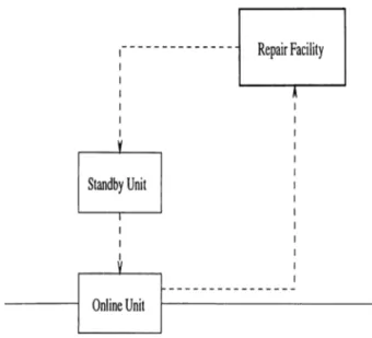
We consider a two-unit redundant cold standby system, with a single repair facility, having exponential service time with rate ¡j,. The lifetime distribution is general. The switchover is immediate. Our aim is to find the optimal replacement age T*, the time interval that minimizes the total costs incurred per unit time, in the long run.

Figure 3.1 depicts the system at hand. Upon failure of the working unit at age x in the time interval [O,?"), the unit is replaced by the standby unit if available, at a cost C f{x ). Unit repair cost is Cr- Preventive maintenance cost of a unit of age x is Cp{x). Denote the service cdf and pdf by H { · ) and h{ · ), respectively, which is exponentially distributed with parameter fi.

Policy 1; At age T, replace the operating unit, even if the other unit is in repair.

Policy 2: At age T, replace the operating unit by the other unit if available; if not available, put off replacement for a while until the other unit returns from repair.

(40)

Figure 3.1: Sketch of the System

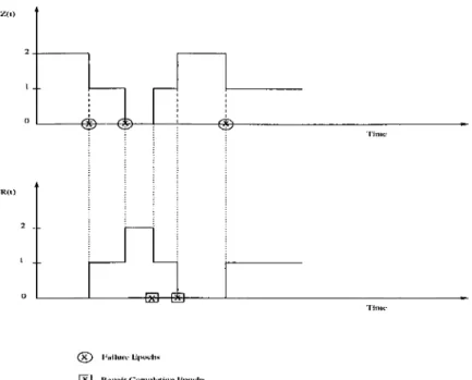
Let > 0} and {R { t) ,t > 0} denote, respectively, the number of

units available and the number of units in the repair facility, at time t. These are stochastic processes, with state spaces

Sz

= {0 ,1 ,2 } and

S

r = {0 ,1 ,2 }.

At any time t > 0, Z (i) + R (t) = 2. This is trivial, since upon failure, the unit is carried to the repair facility in a negligible amount of time; the same is true upon repair completion.

A typical system behavior is illustrated in Figure 3.2.

3.2 THE MARGINAL COST APPROACH

AND ITS MOTIVATION

The Marginal Cost Analysis (M CA) of maintenance policies is a concept gaining more interest in the recent years. This approach has been categorized as an Economics Oriented approach, as different from the classical probability centered approach. The MCA has been successfully applied to the Age Replacement and the Block Replacement policies, and was shown to be flexible enough to permit extensions and generalizations. The M CA concept was introduced by Berg [10] for the solution of maintenance problems. Denote

(41)

^

®

( x ) I'liilui'c Lipoc-hs I X I Repair Completion lipoehs

Figure 3.2: A Typical Realization of the Processes Z(t) and R (t)

by C {T ) the long-run expected cost per unit of time incurred when preventive maintenance is performed at time intervals of length T. Let Vi{x) be the costs incurred if the preventive maintenance is performed at age x. Let 14(3:, A ) stand for the expected costs incurred in (a;, a; + A ] if the preventive maintenance is deferred to age x -|- A (for an infinitesimal A .)

D e fin itio n

10

The Marginal Cost Function (M CF), r]{x), is the cost incurred

if the preventive maintenance action is put off by an infinitesimal amount of time A . That is,

V f i x , A ) - V f f x ) \

nix) = lim ₍

₁

₎

In order to find C{ T) , a renewal process has to be appropriately chosen. Let the renewal interval have a cdf and a pdf denoted by G ( · ) and g{·), respectively. Furthermore, let D{ T) and U{ T) stand for the expected cost during a renewal interval (cycle) and the expected cycle length, respectively. Using the Renewal- Reward Theorem (see e.g. Ross [47]), the long-run expected cost per unit of time, C{ T) , is obtained by dividing the expected cost during a cycle, D{ T) , by the expected cycle length, U{T),

(42)

C{ T) = Dj T)

U(T)

(2)

The aim is to determine T* that minimizes C{ T) , that is, the problem is

m in xC iT ).

There is a theorem from Mathematical Economics, Theorem 1, that makes the MCE a useful and a powerful tool for optimization. Here, we give the theorem, without proof.

T h e o r e m 1 (B e r g [

10

], [11]) The optimal value T* in the problem miny C{ T)

is a solution to the equation

C( T) = , ( T )

₍₃₎

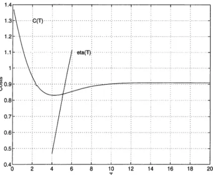
As shown in Figure 3.3, the C{ T) curve is flat in the neighborhood of T*, whereas the r]{T) curve is not. This improves the efficiency of algorithms to solve for T*, if the MCA is used. In addition to that, for the age replacement policy, the M CA has a particular usefulness. Extensions and generalizations are handled by slightly modifying the MCE. The interested reader is referred to Berg [11].

3.3 POLICY 1

Under this policy, at age T, the operating unit is replaced, even if the other unit is in repair. Hence the system is down. In the following derivations, failure cost and preventive maintenance cost are assumed to be independent of time, and are denoted by c / and Cp, respectively. In the marginal cost derivations, however, we allow them to depend on age.

(43)

Figure 3.3: Total costs C (T ), and marginal cost, t]{T), functions versus time

T.