Vol. 1 no. 1 2004Pages 1–10
Pathway Activity Inference Using Microarray Data
O. Babur, E. Demir, A. Ayaz, U. Dogrusoz
∗and O. Sakarya
1Center for Bioinformatics and2Computer Engineering Department, Bilkent
University, Ankara 06533, Turkey
ABSTRACT
Motivation: Microarray technology provides cell-scale ex-pression data; however, analyzing this data is notoriously difficult. It is becoming clear that system-oriented methods are needed in order to best interpret this data. Combining microarray expression data with previously built pathway models may provide useful insight about the cellular ma-chinery and reveal mechanisms that govern diseases.
Given a qualitative state - transition model of the cellular network and an expression profile of RNA molecules, we would like to infer possible differential activity of the other molecules such as proteins on this network.
Results: In this paper an efficient algorithm using a new approach is proposed to attack this problem. Using the regulation relations on the network, we determine possible scenarios that might lead to the expression profile, and qualitatively infer the activity differences of the molecules between test and control samples.
Availability: This new analysis method has been imple-mented as part of a microarray data analysis component within PATIKA (Pathway Analysis Tool for Integration and Knowledge Acquisition), which is a software environment for pathway storage, integration and analysis. Facilities for easy analysis and visualization of the results is also pro-vided.
Contact:http://www.patika.org.
Keywords: Regulatory pathways and networks, gene expression analysis, microarray data analysis, systems biology, pathway activity inference.
INTRODUCTION
Developments in molecular biology research in the past decade resulted in production of vast amount of data. It is possible to conceptualize these data in several layers. At the very bottom lies the genetic code. At the second level, there is information about separate functional units, genes and their encoded products. Compared to the se-quence information, which is simple and uniform, func-tional information is complex and non-uniform. This in-formation is captured in the genome and protein databases such as GeneCards (Rebhan et al., 1997). At the third level
∗To whom correspondence should be addressed ([email protected]).
we consider the system itself. We can think of the second level as a catalogue of parts, and the third level examines how these parts are assembled and work together to per-form the functions of the system. This level is essential to understanding the structure and the function of the molec-ular network carrying out cellmolec-ular processes.
Microarray is a widely used high throughput molecular biology technique, which provides researchers with cell-wide expression profiles. However deriving systemic information from expression profiles remains a big chal-lenge. Activity data of the signaling entities is partially supplied with microarray data. Extending this data to the whole network would be a critical step in system-scale analysis of the cell and may facilitate drug development and bioengineering studies.
In this study, we developed an approach to solve the problem of pathway activity inference, which is the de-termination of activity status of the molecules, using ex-pression profiles. We assume that the underlying cellular network of the subject is already modelled according to the PATIKAontology (Demir et al., 2004). This approach in-puts the differential expressions of genes to assess activity data to RNA molecules and infers activity data for other actors in the network, which are not represented in the mi-croarray data, exploring causal relations between actors.
DEFINITIONS
PATIKA ontology has been designed to model the com-plex molecular network in a cell. Every actor in a cellular process is modelled as a state and every change a state undergoes (e.g. transportation, chemical modification) is called a transition. Different from the convention of rep-resenting different functional forms of a biological entity as a single unit in pathway graphs (entity-level), PATIKA
ontology models them as separate states (state-level). For example tumor suppressor P53 is a biological entity and its p53-DNA, p53-RNA, p53 protein, phosphorylated p53 protein and nuclear p53 protein are all different functional forms and have different responsibilities in the cell. Thus every form is considered to be a distinct state of P53 en-tity. Relations between states and transitions are defined by four type of interactions: substrate, product, activator and inhibitor. Basics of the ontology is illustrated in Fig-ure 1.
Fig. 1. Basics of PATIKA ontology. For instance, Wnt bioentity appears in two different states in this pathway: wnt protein in extracellular matrix and frz-bound wnt protein.
We use the term significant throughout the paper to indicate reliable differential expressions. A significant change describes a change in the expression profiles between control and test samples that satisfies some user defined criteria such as a certain log ratio.
Microarray data supplies the activity status of some RNA states under the experimental conditions. In graphs that have entity-level ontology, expression value of the gene is associated to the representing node as there is no other object to associate the data with. Such graphs are more manageable as far as complexity is concerned, but the hidden details may often leave the analysis blunt. When state-level ontology is used, such as the PATIKA
ontology, RNA state of an entity is represented by a unique node and the data can be associated with RNA states allowing a more precise analysis.
There may be positive (up-regulating) or negative (down-regulating) paths between states, where a regula-tion path is defined as a non-repeating chain of regularegula-tion relations between neighboring states. Positive paths con-tain an even number of inhibitor interactions in the chain, while negative paths contain an odd number of inhibitor interactions. The activity of the first state positively affects the activity of the last state on an up-regulating path. Similarly, the activity of the first state negatively affects the activity of the last state on a down-regulating path.
A regulation graph view is derived from a PATIKAgraph and only represents up and down-regulation relations be-tween states (Figure 2). The substrate and activator inter-actions imply up-regulation, while inhibition interaction implies down-regulation. In the rest of the paper, regula-tion graph views of PATIKAgraphs will be used for sim-plicity.
Fig. 2. A regulation graph view of the PATIKA graph given in Figure 1. Although this looks very similar to entity-level graphs, it is not, as every node represent a different state of a bioentity. Since every state maps to a certain molecule type, semantics of “activates” and “inhibits” relations are unambiguous, they increase and decrease the concentration of that specific state respectively. We also know the level of regulation, whether it is transcriptional or not, a point critical for microarray analysis.
In this study, we tackle the following problem in order to partially infer pathway activity: Given a cellular network with state-level ontology (e.g., a PATIKA graph) and an expression profile of a cell being tested, we would like to determine the activity status of the molecular states in the test cell. We can simply determine the activity status of the significantly changed RNA states from the microarray data. Through the interactions of the cellular network, the expression change of an RNA state may be explained by the expression change of another RNA state. The problem becomes the inference of activity status of the states on the paths between the RNA states with significant expression data, exploring the possible dependency relations in the network.
RELATED WORK
To our knowledge, this study is the first attempt to deduce active pathways by assigning activity status to the nodes of the pathways. There are several other approaches to derive information about the system governing cellular processes using differential expression profiles. Clustering is one of the approaches which attempts to capture the coordinated behaviors between gene expressions. Since coordinated expression of two genes takes place whenever expression of one of them controls the other or they are under control of another common factor, clustering studies reveal information about the actors of a signal flow in the cell. However it is far from determining the order of the flow.
Another similar area is pathway inference, which attempts to discover the gene network structure using the expression profiles. An excellent survey of such work can be found in (D’haeseleer et al., 2003). Please note that pathway inference and pathway activity inference are rather different and in a sense complementary issues since the former tries to build a pathway using expression
profiles while the latter assumes an existing pathway and aims at discovering its active parts given the input expression profile.
There are other studies where the expression data is associated with the underlying pathway structure. Cy-toscape is a software tool, which facilitates visualization of molecular interaction (protein-protein or protein-DNA) networks and can integrate expression data to the network (Ideker et al., 2002). It provides various customizable visualization options to change node color, node label, etc. according to the differential expression values. Cytoscape also reveals connected subnetworks of nodes with high levels of differential expression, which may help user to identify the signaling processes responsible from the changes in the profiles.
GenMAPP is another bioinformatics platform, pro-viding a pathway drawing tool along with a pathway repository (GenMAPP, 2003). Pathways are visualized as mapped static images, which may be colored according to differential expression profiles.
Yet another software tool is ArrayAnalyzer (Krull et al., 2003), which can find pathways between user specified nodes in the TRANSPATH database and color them according to the microarray data. Although TRANSPATH contains limited amount of state-level data, ArrayAnalyzer uses this information only to derive entity-level relations, not for determining the activity or compatibility of the paths.
Vert and Kanehisha (Vert and Kanehisa, 2003) also de-scribe an algorithm to relate microarray data to metabolic pathway graphs. However their notion of pathway is radically different than ours, as in their ontology effec-tors, which are typically proteins, and substrates, which are typically small molecules, form two disjoint sets. Two proteins are neighbors if they catalyze consecutive reactions. They assume that such genes are activated in groups, which is logical for metabolic pathways and lower organisms with multicistronic transcription units. Unfortunately this method cannot be extended to regula-tory pathways in higher eukaryotes where the interplay between genes and their products need to be considered.
In the following sections we describe our algorithm, its implementation and test results.
ALGORITHM
The key idea of our intuitive approach for pathway activity inference is that the regulation of an RNA molecule may be due to another regulated RNA through a regulation path. The algorithm identifies possible differentially active regulation paths between significantly regulated RNA states (significant states in short). We say that a regulation path is compatible with a given microarray data if: • the path is positive and the activity of its start and end
nodes changed in the same direction or
• the path is negative and the activity of its start and end nodes changed in the reverse direction.
The path is called conflicting with the expression data otherwise. Note that the compatibility of the path is only considered when both of its start and end points are significant for the given expression profile.
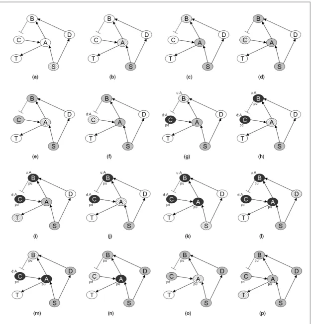
Cyclic chain of regulation relations such as feedback loops poses a problem, as they might lead to false inference. For example in Figure 3 (Lustig et al., 2002), because of feedback inhibition ofβ-catenin complex by Conductin, the path Wnt→ Dsh → Gsk3β complex →
β-catenin complex → Conductin RNA → Conductin →
β-catenin complex is a down-regulation path from Wnt to
β-catenin complex. Butβ-catenin is never down-regulated
by Wnt because the feedback inhibition is only active when there is enough β-catenin complex in the cell.
Negative cycles may lead to false inference where positive cycles does not contribute additional information to the analysis. Therefore, cyclic chains of regulation relations should not be considered during inference.
Fig. 3. Negative feedback loop of Wnt signaling.
Depth-first traversal (DFT) is often used for detecting paths that do not contain a cycle and provides a suitable basis for our algorithm. However, DFT does not consider the compatibility of the traversed path. We may need to traverse over a node twice: one for the positive paths and one for the negative, since that node might be reached from a significant node via both type of paths.
We modify DFT to use two “processed tags” per node instead of one. The current path of traversal implies a regulation from the source node to the visited node (i.e.,
current node), which may be an up or down-regulation.
Traversing the downstream of a node with different regulation types would give different results. On account of this, a different processed tag is used for each regulation type. When a node is re-visited with the other regulation type, its downstream is traversed again.
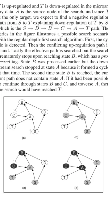
Moreover, DFT as is fails to detect all possible compat-ible regulation paths. A simple example demonstrates this in Figure 4. Here, assumeS andT are significant states,
Sis up-regulated andT is down-regulated in the microar-ray data.S is the source node of the search, and sinceT is the only target, we expect to find a negative regulation path fromS toT explaining down-regulation ofT byS,
which is theS → D → B → C → A → T path. The
series in the figure illustrates a possible search scenario with the regular depth-first search algorithm. First, the cy-cle is detected. Then the conflicting up-regulation path is found. Lastly the effective path is searched but the search prematurely stops upon reaching stateB, which has a
pro-cessed tag. State B was processed earlier but the down-stream search stopped at stateAbecause it formed a cycle at that time. The second time stateB is reached, the cur-rent path does not contain stateA. If it had been possible to continue through statesBandC, and traverseA, then the search would have reachedT.
Fig. 4. Depth-first traversal is not able to find all paths.
This is because when DFT detects a negative cycle, the downstream of the cycle-creating node is not traversed. During backtracking, the nodes on the detected cycle is labelled as processed, and the node which created the cycle can not be visited again through a path containing nodes on the cycle. To overcome this problem, each node on the negative cycle stores a reference to the cycle-creating node as the algorithm backtracks after detection of the cycle. So each node on the graph maintains two
cycle-creating node sets (cycle set in short), one set per
possible regulation of current path. During backtracking, cycle-creating nodes are assigned to the respective cycle sets. When a node on the previously traversed negative cycle is visited again, its related cycle set is checked and if the set contains any node which is not on the current
path, this node is removed from the set and downstream of current node is re-traversed.
The algorithm runs for each significant node of the graph, using it as the source node of the traversal towards multiple targets. When a microarray compatible regulation path is found between the source and another significant state (target), the up or down-regulation of the states on the regulation path is inferred. During an execution for a source, the inferences for other sources are not considered. A state may be inferred as both up and down-regulated through different regulation paths. Identification of the more likely activity is a complicated task and is not addressed here. The inference algorithm is more formally given below.
algorithmINFER ALL(graph) (1) for (each node of graph)
(2) callINFER FOR SOURCE(node)
algorithmINFER FOR SOURCE(source node)
(1) if (regulation type of source node is up-regulation) (2) effect of path := up-regulation
(3) else
(4) effect of path := down-regulation
(5) initialize current path as an empty list (6) output callINFER REC(source node,
source node, effect of path, current path)
algorithmINFER REC(source node, current node,
effect of path, current path) returns cycle set
(1) // Check if the current node creates a cycle. (2) if (current node in current path) // cycle detected (3) if (current node not “processed” for effect of path
or “inferred” for effect of path) (4) return current node in a set
(5) else
(6) return empty set
(7) // Check if any inference is possible.
(8) if (current node “inferred” for effect of path or “significant”)
(9) if (callPATH IS COMPATIBLE(source node,
current node, effect of path))
(10) callINFER PATH(current path)
(11) return empty set // stop traversing further (12) // Check if the current node is already “processed”. (13) if (current node “processed” for effect of path) (14) if (cycle set of current node for effect of path
contains elements outside current path) (15) remove elements outside current path
from the cycle set (16) else
(17) return cycle set of current node for effect of path
(18) // Traverse the current node. (19) add current node to current path
(20) for (each child child node of current node) (21) new effect of path :=
callGET NEW EFFECT OF PATH(
current node, child node, effect of path)
(22) returned cycle set :=
callINFER REC(source node, child node,
new effect of path, current path)
(23) if (current node not “inferred” for effect of path and not “significant”)
(24) remove current node if in returned cycle set (25) add nodes of returned cycle set to the
cycle set of current node for effect of path
(26) remove current node from current path (27) label current node as “processed”
for the effect of path
(28) return cycle set of current node for effect of path algorithmPATH IS COMPATIBLE(
source node, current node, effect of path)
(1) if (current node is “significant”) (2) if (regulation type of source node = (3) regulation type of current node) (4) if (effect of path is down-regulation)
(5) return false
(6) else // regulation types are different (7) if (effect of path is up-regulation)
(8) return false
(9) return true
algorithmGET NEW EFFECT OF PATH(
current node, child node, effect of path)
(1) if (current node “up-regulates” child node) (2) direct regulation := up-regulation
(3) else
(4) direct regulation := down-regulation
(5) if (effect of path is up-regulation) (6) return direct regulation (7) else
(8) return negation of direct regulation algorithmINFER PATH(path)
(1) current node := last node of path (2) while (current node not “significant”
and not “inferred” for the effect of
path on current node)
(3) label current node with
the effect of path on current node (4) current node := parent of current node
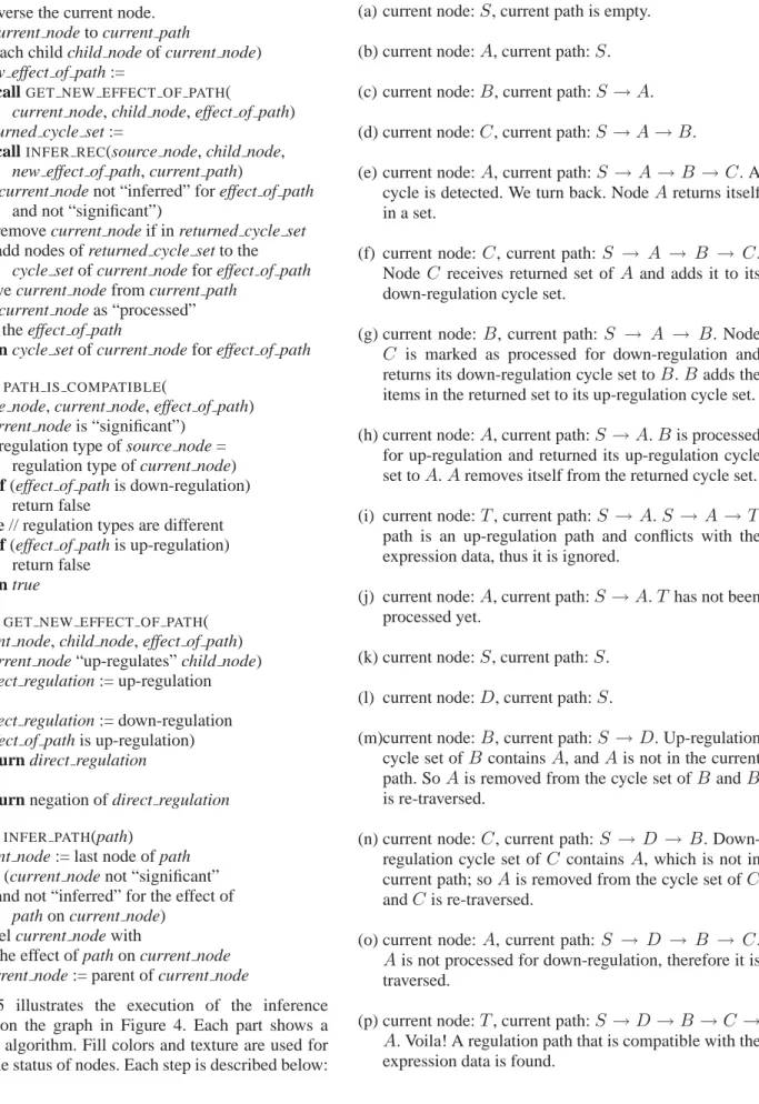
Figure 5 illustrates the execution of the inference algorithm on the graph in Figure 4. Each part shows a step of the algorithm. Fill colors and texture are used for showing the status of nodes. Each step is described below:
(a) current node:S, current path is empty. (b) current node:A, current path:S. (c) current node:B, current path:S → A. (d) current node:C, current path:S → A → B.
(e) current node:A, current path:S → A → B → C. A cycle is detected. We turn back. NodeAreturns itself in a set.
(f) current node:C, current path:S → A → B → C. NodeC receives returned set of Aand adds it to its down-regulation cycle set.
(g) current node:B, current path: S → A → B. Node C is marked as processed for down-regulation and returns its down-regulation cycle set toB.B adds the items in the returned set to its up-regulation cycle set. (h) current node:A, current path:S → A.Bis processed
for up-regulation and returned its up-regulation cycle set toA.Aremoves itself from the returned cycle set. (i) current node:T, current path:S → A.S → A → T path is an up-regulation path and conflicts with the expression data, thus it is ignored.
(j) current node:A, current path:S → A.Thas not been processed yet.
(k) current node:S, current path:S. (l) current node:D, current path:S.
(m)current node:B, current path:S → D. Up-regulation cycle set ofB containsA, andAis not in the current path. SoAis removed from the cycle set ofBandB is re-traversed.
(n) current node:C, current path:S → D → B. Down-regulation cycle set ofC contains A, which is not in current path; soAis removed from the cycle set ofC andCis re-traversed.
(o) current node:A, current path:S → D → B → C. Ais not processed for down-regulation, therefore it is traversed.
(p) current node:T, current path:S → D → B → C → A. Voila! A regulation path that is compatible with the expression data is found.
Fig. 5. A demonstration of the inference algorithm on a sample cyclic graph. Nodes on the current path are filled with gray and current
node with texture. Processed nodes (for up or down-regulation) are filled with black. Whenever more than one color is possible for a node, the priority order is: textured, gray and black. The processed tags are also shown on the bottom-right of the nodes (pd: processed for down-regulation, pu: processed for up-regulation). The elements of cycle sets is shown on the top-right of nodes (u:X denotes cycle set for up-regulation contains node X, d:X denotes cycle set for down-regulation contains node X). Each figure illustrates a step in the algorithm as described in the text.
Time Complexity
Inference algorithm is based on DFT and has identical time complexity when there are no cycles in the graph. If the source node can reach all the other nodes, DFT visits all nodes and edges. Inference algorithm uses two
processed tags for the nodes (instead of one used in regular
DFT). Thus each node and edge can be traversed twice in
the worst case, leading to a complexity ofO(|V | + |E|), where|V |is the number of nodes and|E|is the number of edges in the pathway graph.
When the graph is cyclic, a processed node may be re-traversed because of the nodes in its cycle sets. The algorithm keeps track of cycle-creating nodes, that are inferred or not processed for the current regulation type.
During backtracking, cycle-creating node is inserted into the respective cycle set of the other nodes on the cycle. If the algorithm later reaches a processed node with a non-empty cycle set, it may re-traverse the node, in order to re-reach the members of the set.
A cycle-creating node is removed from the cycle set of another node when the node owning the set is re-traversed because of the cycle-creating node. Note that once a node is removed it will never be re-inserted to the same cycle set. The reasoning follows.
The tags processed, inferred and cycle set are used related to the current regulation types of nodes in this paragraph. Suppose node B contains nodeAin its cycle set. IfBis re-traversed due toAthenAcan not appear on the upstream ofBin the current path. Therefore,Acannot create a cycle containingBduring this traversal. After the traversal ofB, if an inference is done upon reachingA,B will also be inferred and will not be traversed anymore for the current regulation type. If no inference is done, thenA will be tagged as processed, thus can not be inserted into any cycle set.
In the worst case each node would have all the other nodes in its cycle sets and will remove just one of them in each traversal. |V | − 1 nodes in sets will result in |V | − 1 traversals per cycle set, a total of 2(|V | − 1) traversals per node. In order to check whether a cycle set contains elements outside the current path, the algorithm will consider an average of(|V |−1)/2nodes in the worst case. Thus the total complexity of the traversal for a single source sums up to
O((|V | − 1)22(|V | + |E|)) = O(|V |3+ |E||V |2). Suppose there are|S|significant states on the graph, then the traversal will be executed |S| times, therefore the resulting complexity is
O(|S|(|V |3+ |E||V |2)).
Since the highest possible value of|E| is|V |(|V | − 1), the algorithm has a quartic complexity. However, there is growing evidence supporting the fact that biological networks are scale-free (Rzhetsky and Gomez, 2001), which implies that |E| is proportional to |V | and the average size of cycle sets is a constant. Thus re-traversals and check of cycle sets can be assumed to take constant time, lowering our worst case upper bound to linear. This upper bound complies with our experimental results described in the next section.
Implementation
PATIKA An integrated environment for cellular path-way data analysis and collaborative construction named PATIKA incorporates a graph model based on PATIKA
ontology as described earlier. It has a client side visual
editor for pathway construction and analysis. A server side component provides query and submission services to the users. PATIKA server employs a concurrency
system in order to coordinate submission process and merge models submitted by users to a single large model.
Microarray Analysis Facility Microarray data do not have a standard file format yet. PATIKAcurrently supports Stanford Microarray Database data format (Gollub et al., 2003). This is a tab delimited text file format, where each row represents a gene.
The gene symbol, which is used to identify genes, is supplied by Human Genome Organization (HUGO) Gene Nomenclature Committee (HUGO, 2003). Since gene symbol is used as the primary name of biological entities in PATIKA database, mapping the expression data to the PATIKAbioentities is usually a straightforward process.
Since the reliability of microarray data can be quite low, a facility for filtering out non-reliable data is essential. PATIKA allows user to define custom set of filters, and only the data rows that satisfy all the filters are accepted as significant. Each significant row of the microarray data is mapped to the RNA states of the related biological entity.
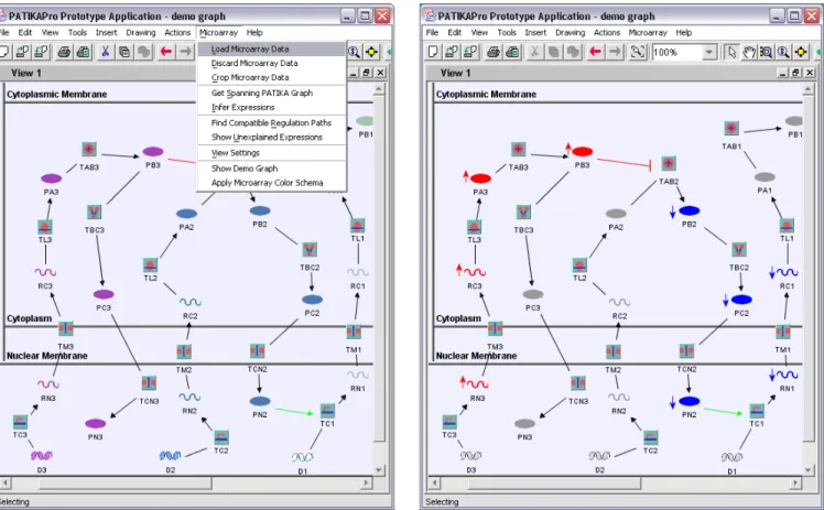
Figure 6 shows a sample demo graph. When the user selects “load microarray data” option in the “microarray” menu, the selected file is loaded and a filter dialog is displayed (Figure 7) to let the user define filters for the trusted microarray data. Figure 8 shows the activity inferred based on the provided microarray data. Here, with the help of the RNA-level data provided by the microarray data, the algorithm is able to infer possible activity of protein states.
Inference and Other Analysis Tools The RNA states of the spanning graph are automatically associated with expression data. At this point data associated is expected to be sparse, since only a subset of the RNA states are significant. After running the inference algorithm on the graph, inferred activity status of nodes is displayed. User is provided with visualization facilities such as coloring schemas and multiple views to examine the inferred differential activity.
Even a visual inspection of the resulting graph may provide the user with useful insight about the mechanisms active in test cells. In addition to the created view, the editor supports some helpful facilities for the analysis: • Highlighting the RNA states whose expression can not
be explained by other expressions.
• Highlighting the up-regulator states of a state. • Highlighting the down-regulator states of a state. • Highlighting the states that are up-regulated by a state.
Fig. 6. Demo graph displayed by the PATIKA editor before microarray data is loaded.
Fig. 7. The filter dialog for microarray data. The filtered microarray
data is mapped to the current graph as input to the inference algorithm.
• Highlighting the states that are down-regulated by a state.
Fidelity Test
We would be able to test our results through inferring a part of significant states, using the rest of the significant states, if we had a large scale cellular model at the desired level of detail. Unfortunately, such models are not available at the present. Instead we opt to demonstrate that the outcomes of our algorithm is sensible, through a theoretical model.
Fig. 8. The inferred activity is highlighted (blue: down-regulated,
red: up-regulated) and up and down-regulated nodes on the active
path are marked with up and down arrows, respectively by the algorithm.
First of all, a hypothetical testing graph, i.e. an artificial large scale cellular model, is created. The structure of the hypothetical graph is designed to capture the real observed patterns and relations as much as possible, such as transcriptional regulations, complex formations, post-translational modifications, etc.
In order to emulate microarray data, we assumed that a state’s activity is either on or off that tells if the molecule exists in the cell effectively. The control case is generated by assigning on values to a high percentage of the DNA states and propagating the activity to the neighboring states, according to the regulation type of the edges. The transitions with known inputs are given priority. Moreover, conflicts and errors are also introduced with a low probability to capture the unknown events and experimental errors. The test case is generated by introducing a single change in the activity of one of the DNA states, and disseminating its effect throughout a portion of the network. While propagating the effect we use the same constraints that are used in generating the
control case.
Afterwards, the microarray data is generated by check-ing a subset of RNA molecules. If their expression status differs in the control and test cases, they are assumed to be significant states of the microarray experiment. Finally, the inference algorithm is executed on the network and the results are compared with the activity data of the test case. The hypothetical graph is constructed with 500 bioen-tities,∼3000 states,∼4400 up-down regulation relations. After creation of the control case, test case is created by changing activity status of 500 states, starting from a DNA molecule, propagating through regulation relations.
Average results of 50 trials showed that about 110 states among 500 affected states is inferred with 95% accuracy. Besides the affected states, unaffected states on alternative compatible paths between significant RNAs are also inferred (Figure 9).
Fig. 9. Pie chart showing the percentage of different inferences. The
inference is on the correct path with a probability of 0.55. When on the correct path, its activity status is inferred with high accuracy.
DISCUSSION AND CONCLUSION
We believe that the pathway activity inference is an important problem, as it examines the activity status of the molecular states in the cells being tested, as opposed to the underlying static relations (e.g., those described by PATIKAgraphs). Obviously our solution is not a complete one, however it provides a necessary initial step by finding paths on the network graph that are compatible with the given expression profile.
Although the results of theoretical testing is promising, it is far from being a proof of concept. Testing our algorithm with real biological data is our next step, which would allow us to pinpoint possible problems and improve our algorithm. Our major bottleneck is the lack of system-scale static models. PATIKAprovides us with a convenient framework for collaboratively constructing such a model. Fortunately new high throughput methods (Zhu et al., 2001; Ito et al., 2001), databases (Bader et al., 2001; Xenarios et al., 2001; Karp et al., 2002), data exchange
formats (Ashburner et al., 2000; Hucka et al., 2003; BioPAX, 2003) and computational methods (Hvidsten et al., 2001; Akutsu et al., 2000; Segal et al., 2003) are being developed at an amazing rate and we expect to have system-scale models of human cells in the near future.
Building a static model is a one-time task. On the other hand examining the dynamic status of the system is a recurring task, as the possible number and combinations of deviations, from the “normal” system is virtually infinite. In cases such as cancer, such deviations could be different for each patient. The algorithm lines out possible scenarios that might explain changes in the microarray data, and may help to discover such polymorphisms, diseases or abnormalities. Choosing the most likely scenario is one of the most challenging tasks for future research.
An interesting application of the algorithm arises when a single parameter is changed between control and the test such as a mutation or a chemical in the medium in the expression profiling experiment. This initial change in turn will modify the status of certain states, some of which can be measured directly via microarray experiments. Since no other parameter was changed in the system, changes in the expression profile must be somehow associated with the initial difference. Therefore any affected state must be reachable in our graph from the initial state, through a path that does not conflict with the microarray data. If it is not reachable, then we can deduce that there is an experimental error or a path missing in our graph. If there is a single non-conflicting path from initial state to affected state then we can infer the status of every node on this path. Note that this deduction represents the most likely explanation in our best knowledge. If there are multiple paths from the source to the target, then there can be two possibilities for each path. They can be effectual paths, meaning that their effect is partially or completely responsible for the observed change of their target. Alternatively, they can be ineffectual, meaning that they are not responsible for the observed change since their effect on the target is dominated by at least one effectual path.
Although the algorithm has not been tested with real biological data yet, we expect to have multiple effectual paths on a certain target. A well-known example is com-plementary pathways, in which a signal is propagated in two parallel paths (Haupt et al., 2003). On the bright side, this algorithm can potentially discover such complemen-tary relations between paths as well.
Our experiments show that inference on ineffectual paths are not likely to return correct results. Therefore it is necessary to be able to separate ineffectual paths from effectual ones. One method is through expert examination. An expert can separate paths that are likely to be effectual considering the properties of the path. Moreover they can conduct specific experiments to investigate ambiguous
points. Obviously, other high throughput techniques, which can assess the status of states other than RNAs would be of great help and would significantly reduce the ambiguities in the analysis. It is possible to improve the accuracy of inference by using the algorithm to assign activities to the states on unambiguous points, and use these new assignments to rule out some ineffectual paths, until no new inference can be made.
If such methods can produce system-scale dynamic models, we will need to capture and integrate this data. Pathway ontologies will need to be extended to capture sequence of signal flow, stochastic alternatives and dom-ination rules that are not necessarily evident from the topology of the static model.
REFERENCES
Akutsu, T., S. Miyano, and S. Kuhara (2000). Inferring qualitative relations in genetic networks and metabolic pathways.
Bioinfor-matics 16(8), 727–734.
Ashburner, M., C. Ball, J. Blake, D. Botstein, H. Butler, J. C. JM, A. Davis, K. Dolinski, S. Dwight, J. Eppig, M. Harris, D. Hill, L. Issel-Tarver, A. Kasarskis, S. Lewis, J. Matese, J. Richardson, M. Ringwald, G. Rubin, and G. Sherlock (2000, May). Gene ontology: tool for the unification of biology. the gene ontology consortium. Nat. Genet. 25(1), 25–29.
Bader, G., I. Donaldson, C. Wolting, B. Ouellette, T. Pawson, and C. Hogue (2001). Bind-the biomolecular interaction network database. Nucleic Acids Research 29, 242–245.
BioPAX (2003). Biological pathways exchange.
http://www.biopax.org.
Demir, E., O. Babur, U. Dogrusoz, A. Gursoy, A. Ayaz, G. Gulesir, G. Nisanci, and R. Cetin-Atalay (2004). An ontology for collaborative construction and analysis of cellular pathways. To appear in Bioinformatics.
D’haeseleer, P., S. Liang, and R. Somogyi (2003). Genetic network inference: from co-expression clustering to reverse engineering.
Bioinformatics 16, 707–726.
GenMAPP (2003). Gene microarray pathway profiler.
http://www.genmapp.org.
Gollub, J., C. Ball, G. Binkley, J. Demeter, D. Finkelstein, J. Hebert, T. Hernandez-Boussard, H. Jin, M. Kaloper, J. Matese, M. Schroeder, P. Brown, D. Botstein, and G. Sherlock (2003, Jan-uary). The stanford microarray database: data access and quality assessment tools. Nucleic Acids Res. 31(1), 94–6.
Haupt, S., M. Berger, Z. Goldberg, and Y. Haupt. (2003, October). Apoptosis - the p53 network. J Cell Sci. 116, 4077–85. Hucka, M., A. Finney, H. M. Sauro, H. Bolouri, J. C. Doyle,
H. Kitano, A. P. Arkin, B. J. Bornstein, D. Bray, A. Cornish-Bowden, A. A. Cuellar, S. Dronov, E. D. Gilles, M. Ginkel, V. Gor, I. I. Goryanin, W. J. Hedley, T. C. Hodgman, J.-H. Hofmeyr, P. J. Hunter, N. S. Juty, J. L. Kasberger, A. Kremling, U. Kummer, N. Le Novere, L. M. Loew, D. Lucio, P. Mendes, E. Minch, E. D. Mjolsness, Y. Nakayama, M. R. Nelson, P. F. Nielsen, T. Sakurada, J. C. Schaff, B. E. Shapiro, T. S. Shimizu, H. D. Spence, J. Stelling, K. Takahashi, M. Tomita, J. Wagner, and J. Wang (2003). The systems biology markup
language (SBML): a medium for representation and exchange of biochemical network models. Bioinformatics 19(4), 524–531. HUGO (2003). Hugo gene nomenclature committee. World Wide
Web. http://www.gene.ucl.ac.uk/nomenclature/.
Hvidsten, T. R., J. Komorowski, A. K. Sandvik, and A. Laegreid (2001). Predicting gene function from gene expressions and ontologies. In Pacific Symposium on Biocomputing, pp. 299–310. Ideker, T., O. Ozier, B. Schwikowski, and A. Siegel (2002). Discovering regulatory and signaling circuits in molecu-lar interaction networks. Bioinformatics 18, S233–S240.
http://www.cytoscape.org/.
Ito, T., T. Chiba, R. Ozawa, M. Yoshida, M. Hattori, and Y. Sakaki (2001). A comprehensive two-hybrid analysis to explore the yeast protein interactome. Proceedings of the National Academy
of Sciences 98, 4569–4574.
Karp, P., S. Paley, and P. Romero (2002). The pathway tools software. Bioinformatics 18, S225–232.
Krull, M., N. Voss, C. Choi, S. Pistor, A. Potapov, and E. Wingender (2003). TRANSPATH(R): an integrated database on signal transduction and a tool for array analysis. Nucl. Acids. Res. 31(1), 97–100.
Lustig, B., B. Jerchow, M. Sachs, S. Weiler, T. Pietsch, U. Karsten, M. van de Wetering, H. Clevers, P. Schlag, W. Birchmeier, and J. Behrens (2002, February). Negative feedback loop of wnt signaling through upregulation of conductin/axin2 in colorectal and liver tumors. Molecular and Cellular Biology 22(4), 1184– 1193.
Rebhan, M., V. Chalifa-Caspi, J. Prilusky, and D. Lancet (1997). GeneCards: encyclopedia for genes, proteins and diseases. http://bioinformatics.weizmann.ac.il/cards/.
Rzhetsky, A. and S. M. Gomez (2001). Birth of scale-free molecular networks and the number of distinct DNA and protein domains per genome. Bioinformatics 17(10), 988–996.
Segal, E., M. Shapira, A. Regev, D. Pe’er, D. Botstein, D. Koller, and N. Friedman (2003). Module networks: identifying regula-tory modules and their condition-specific regulators from gene expression data. Nature Genetics 34, 166–76.
Vert, J. and M. Kanehisa (2003). Extracting active pathways from gene expression data. Bioinformatics 19(90002), 238ii–244. Xenarios, I., E. Fernandez, L. Salwinski, X. Duan, M. Thompson,
E. Marcotte, and D. Eisenberg (2001). Dip: The database of interacting proteins: 2001 update. Nucleic Acids Research 29(1), 239241.
Zhu, H., M. Bilgin, R. Bangham, D. Hall, A. Casamayor, P. Bertone, N. Lan, R. Jansen, S. Bidlingmaier, T. Houfek, T. Mitchell, P. Miller, R. Dean, M. Gerstein, and M. Snyder (2001). Global analysis of protein activities using proteome chips. Science 293, 2101–2105.