Quadratic assignment problem : linearizations and polynomial time solvable cases

(1)

QUADRATIC ASSIGNMENT PROBLEM:

LINEARIZATIONS AND POLYNOMIAL TIME

SOLVABLE CASES

A THESIS

SUBMITTED TO THE DEPARTMENT OF INDUSTRIAL ENGINEERING AND THE INSTITUTE OF ENGINEERING AND SCIENCE

OF BILKENT UNIVERSITY

IN PARTIAL FULFILLMENT OF THE REQUIREMENTS FOR THE DEGREE OF

DOCTOR OF PHILOSOPHY

By Güneş Erdoğan

(2)

I certify that I have read this thesis and that in my opinion it is fully adequate, in scope and in quality, as a dissertation for the degree of Doctor of Philosophy.

___________________________________ Prof. Barbaros Tansel (Supervisor)

___________________________________ Prof. Cevdet Aykanat

___________________________________ Prof. Erhan Erkut

___________________________________ Assoc. Prof. Levent Kandiller

___________________________________ Assist. Prof. Hande Yaman

Approved for the Institute of Engineering and Science:

___________________________________ Prof. Mehmet Baray

(3)

ABSTRACT

QUADRATIC ASSIGNMENT PROBLEM: LINEARIZATIONS

AND POLYNOMIAL TIME SOLVABLE CASES

Güneş Erdoğan

Ph.D. in Industrial Engineering Supervisor: Prof. Barbaros Tansel

October 2006

The Quadratic Assignment Problem (QAP) is one of the hardest combinatorial optimization problems known. Exact solution attempts proposed for instances of size larger than 15 have been generally unsuccessful even though successful implementations have been reported on some test problems from the QAPLIB up to size 36. In this dissertation, we analyze the binary structure of the QAP and present new IP formulations. We focus on “flow-based” formulations, strengthen the formulations with valid inequalities, and report computational experience with a branch-and-cut algorithm. Next, we present new classes of instances of the QAP that can be completely or partially reduced to the Linear Assignment Problem and give procedures to check whether or not an instance is an element of one of these classes. We also identify classes of instances of the Koopmans-Beckmann form of the QAP that are solvable in polynomial time. Lastly, we present a strong lower bound based on Bender’s decomposition.

Keywords: Quadratic Assignment Problem, Linearization, Computational Complexity, Polynomial Time Solvability

(4)

ÖZET

KARESEL ATAMA PROBLEMİ: DOĞRUSALLAŞTIRMALAR

VE POLİNOM ZAMANDA ÇÖZÜLEBİLİR DURUMLAR

Güneş Erdoğan

Endüstri Mühendisliği Bölümü Doktora Tez Yöneticisi: Prof. Barbaros Tansel

Ekim 2006

Karesel Atama Problemi (KAP) bilinen en zor kombinatoryal eniyileme problemlerinden biridir. QAPLIB’deki boyutu 36’yı bulan bazı test problemlerinde başarılı çözümler elde edilmiş olsa da, tam çözüm yöntemleri boyutu 15’i geçen problemlerde genel olarak başarısız olmuştur. Bu tezde, KAP’ın ikili yapısını inceleyip yeni tamsayı programlar sunmaktayız. “Akış-tabanlı” formülasyonlara odaklanıp, bunları geçerli eşitsizliklerle kuvvetlendirip, dallan-ve-kes algoritması ile edindiğimiz hesapsal tecrübeyi sunmaktayız. Devamla, KAP’ın Doğrusal Atama Problemine tamamen veya kısmen indirgenebilen özel hallerini sunmakta ve verilen bir problemin bu sınıfların bir elemanı olup olmadığını kontrol eden prosedürler vermekteyiz. Ayrıca KAP’ın Koopmans-Beckmann formuülasyonunun polinom zamanda çözülebilir sınıflarını ortaya çıkartmaktayız. Son olarak, Bender ayrışımına dayanan kuvvetli bir alt sınır sunmaktayız.

Anahtar Kelimeler: Karesel Atama Problemi, Doğrusallaştırma, Hesaplama Zorluğu, Polinom Zamanlı Çözülebilirlik

(5)

(6)

ACKNOWLEDGEMENTS

I thank my advisor Prof. Barbaros Tansel for his guidance, expertise, and patience throughout this dissertation research. With his support, this study has been an invaluable learning experience for me. It has really been an honor to work with this consummate professional.

I am indebted to members of my dissertation committee, Prof. Cevdet Aykanat, Prof. Erhan Erkut, Assoc. Prof. Levent Kandiller, and Assist. Prof. Hande Yaman, for showing keen interest in the subject matter and for accepting to read and review this thesis. Their remarks and recommendations have been invaluable.

It may be unusual to thank an institution; nevertheless I feel the need to thank Bilkent University for providing such an excellent environment for self-development. After 4 years of B.S., 2 years of M.S., and 5 years of Ph.D. study, I ask myself: If there was a higher degree of education, would I pursue it at Bilkent University? The answer is yes, without hesitation.

I would like to express my thanks to my colleagues at Tepe Teknoloji Inc., Babur Baturay, Fatih Canpolat, Menderes Fatih Güven, Nejat Serpen, Osman Tufan Doğan, and Veli Biçer for their help and support during the last phase of my graduate study.

I also would like to express my special thanks to my friends Başar Uncu, Bedrettin – Zeynep Duran, Burç Uzman, Burkay Genç, Emre Can Sezer, İlker – Esra Yağlıdere, Kağan Menekşe, Kamer Kaya, Murat Güler, Özgür Kutluözen, Selim Akgül, Serkan Bayraktar, Sibel Alumur, and Tayfun Küçükyılmaz for their help and morale support.

Finally, I would like to express my deepest gratitude to all members of my family, especially my mother Şenol Erdoğan, for their love, understanding, and patience.

(7)

LIST OF FIGURES

Figure 1. Computational Progress for Instances of Nugent, Vollmann, and Ruml

...3

Figure 2. An Example of Assignment Matrix...15

Figure 3. Pairwise Assignment Matrix and its Submatrices ...16

Figure 4. Lawler’s Linearization ...19

Figure 5. Kaufman and Broeckx’s Linearization ...20

Figure 6. Balas and Mazzola’s Linearization ...21

Figure 7. An Overview of the Literature ...23

Figure 8. Multicommodity Flow Formulation...24

Figure 9. Multicommodity Distance Formulation...28

Figure 10. Single Commodity Flow Formulation...28

Figure 11. Single Commodity Distance Formulation...32

Figure 12. Facility-Based Formulation...33

Figure 13. Location-Based Formulation...34

Figure 14. Facility-Location Formulation...35

Figure 15. A Final View of the Literature...39

Figure 16. Flow Diagram for the Proposed Branch-and-Cut Algorithm...50

Figure 17. Hamiltonian Path on a Grid Graph (a is odd)...88

Figure 18. Hamiltonian Cycle on a Grid Graph (a is even)...91

(10)

LIST OF TABLES

Table 1. Computational Results...37

Table 2. Effect of Valid Inequalities on Lower Bound...53

Table 3. Problems Solved to Optimality by Branch-and-Cut...55

Table 4. Suboptimally Solved Problems...58

Table 5. Comparison of scaled CPU times (in minutes) for instances nugxx...59

Table 6. Run Times with Different Initial Upper Bound Values...60

Table 7. Indices Computed for the Instances from QAPLIB...60

Table 8. Deviations of the objective function values of the solutions obtained by solving the closest element of Class 1, from the optimal objective function values ...75

Table 9. Computational results for the branch-and-cut algorithm using Kaufman-Broeckx formulation, and the proposed valid inequalities ...105

(11)

C h a p t e r 1

INTRODUCTION

The Quadratic Assignment Problem (QAP) was introduced by Koopmans and Beckmann in 1957 as a mathematical model for the location of a set of indivisible economic activities. The decision to be made is a one-to-one assignment of n facilities to n locations, which is exactly the same as the Linear Assignment Problem (LAP) except for the objective function. The term “quadratic” describes the cost function, which is the sum of the products of distances between locations and the amounts of flows between the facilities assigned to the locations.

Generating a feasible solution for the QAP is a trivial task. Let a = (a(1), a(2), …, a(n)) be a permutation of the integers {1,...,n} with a(i) denoting the index of the location to which facility i is assigned. Any such vector a is a feasible solution to the QAP. Similarly, devising a heuristic for the QAP is not a major task. A greedy k-exchange algorithm that starts with a random assignment is a valid (and surprisingly high quality) heuristic for the QAP. On the contrary, proving computationally the optimality of a given solution is next to impossible for large instances of the QAP. It has been shown that the QAP is NP-Hard in the strong sense (Sahni and Gonzales, 1976).

Despite 49 years of academic effort, from its initial formulation in 1957 to date, it remains as yet one of the hardest combinatorial optimization problems. Even though faster computers, specialized data structures, and algorithmic improvements have led to significant progress in solvable sizes of many NP-Hard problems (e.g. the Traveling Salesman, Vehicle Routing, Set Covering,

(12)

Uncapacitated Facility Location, etc.), the QAP has been defiantly resisting all solution attempts beyond the size of n > 15 when the cost data is arbitrary. The largest solved instance of the QAP to date is of size 36 (Nyström, 1999; Brixius and Anstreicher, 2001) while the largest solved size of, for example, the Traveling Salesman Problem has close to 25000 cities (Applegate et al., 2001).

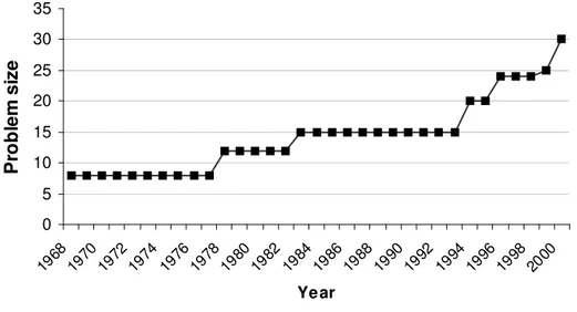
For a better understanding of the current computational status of the QAP, we now give a historical sketch of the computational progress. A collection of instances and respective solutions, QAPLIB (Burkard, Karisch, and Rendl, 1997), is available online to benchmark efficiency of solution methods for the QAP. Although many different classes of instances exist in the QAPLIB, the computational improvement for the QAP may best be explained by the progress in solving the notoriously difficult instances of Nugent, Vollmann, and Ruml (1968). These are the most used instances for testing computational efficiency. The original set consists of 8 instances of sizes 5, 6, 7, 8, 12, 15, 20, and 30. Distance matrices for sizes 5 and 7 represent almost rectangular grid graphs. For sizes 6, 8, 12, 15, 20, and 30, the distance matrix represents grids of 2*3, 2*4, 3*4, 3*5, 4*5, and 5*6, respectively. Later, instances of sizes 14, 16, 17, 18, 21, 22, 24, and 25 were added to the original set by Clausen and Perregaard (1997) by deleting certain rows and columns of flow and distance matrices of larger instances. Likewise, Anstreicher et al. (2002) constructed instances of sizes 27 and 28 in the same way.

Nugent, Vollmann, and Ruml (1968) solved instances nug05, nug06, nug07, and nug08 to optimality using complete enumeration. Burkard and Stratmann (1978) solved nug12 and Burkard and Derigs (1983) solved nug15. Clausen and Perregaard were able to solve instances up to size 20 for the first time in 1994. Their results were published in 1997. Bruengger et al. were the first ones to solve nug21 and nug22 in 1996. In the same year, Clausen et al. reportedly solved nug24. Marzetta and Brüngger managed to solve nug25 in

(13)

1999. Finally, Anstreicher et al. (2002) were able to solve nug27, nug28, and nug30 to optimality in the year 2002. The progress is summarized in Figure 1.

0 5 10 15 20 25 30 35 19 68 19 70 19 72 19 74 19 76 19 78 19 80 19 82 19 84 19 86 19 88 19 90 19 92 19 94 19 96 19 98 20 00 Ye ar P ro b le m s iz e

Figure 1: Computational Progress for Instances of Nugent, Vollmann, and Ruml

This set of instances is not fully representative of the overall computational state of the art for the QAP. As of this writing, the largest instances reportedly solved are ste36a, ste36b, and ste36c that are of size 36. These instances were proposed by Steinberg in 1961. Solving ste36a required 180 hours on a PIII 800 Mhz PC, while ste36b and ste36c took approximately 60 days and 200 days of CPU time, respectively. However, instances proposed by Burkard and Offermann in 1977 of size 26 have remained unsolved until recently (March 2004), at which time they were solved by the method of Hahn et al. (2001). There are still instances of size 30 waiting to be solved in the QAPLIB. We emphasize the fact that most successful applications are parallel implementations that rely on high amounts of computing power.

(14)

The computational status of the QAP poses a challenge: What new perspectives do we need to solve larger sizes of the QAP without having to rely on the high computing power of parallel processing? In this dissertation we pick up the challenge and devise an exact solution technique for the QAP that can solve large instances in a reasonable amount of computing time. Our search for such techniques has led us to identify instances which can be solved in polynomial time, which we also present.

We start by giving the formal definition of the QAP.

1. 1 Problem Definition

Although a brief description of the problem was given in the beginning of the chapter, we believe that the QAP can best be expressed in terms of compact formulations. The original formulation of the QAP by Koopmans and Beckmann (1957), where the decision variable xij is defined to be equal to 1 if facility i is

assigned to location j and 0 otherwise, follows:

ij n j i ij n l k j i kl ij jl ikd x x c x f

∑

= = + 1 , 1 , , , min (1) s.t. n i x n j ij 1, 1,..., 1 = ∀ =

∑

= (2) n j x n i ij 1, 1,..., 1 = ∀ =

∑

= (3)

{ }

i j n x_ij ∈ 0,1,∀, =1,..., (4)

where fik denotes the amount of flow between facilities i and k, djl denotes the

(15)

location j. The linear cost coefficients may be added to certain quadratic cost coefficients to yield a pure quadratic problem and were ignored in later studies.

Lawler (1963) studied the case of generalized cost coefficients where a four dimensional matrix that defines all the costs is the input data instead of two n by n coefficient matrices. The following is the formulation for the Lawler QAP:

∑

= n l k j i kl ij ijklx x C 1 , , , min (5) s.t. (2), (3), and (4)

where Cijkl denotes the cost incurred when facility i is located at j and facility k is

located at l simultaneously.

A third formulation by Edwards (1977), also known as the trace formulation and is useful for certain derivations, is as follows:

)

(

min

T T

X∈Π

tr

FXD

X

(6)

where F is the n by n flow matrix, D is the n by n distance matrix, X is an n by n permutation matrix, ∏ represents the set of n by n permutation matrices, and

R R

tr: n2 → is the trace operator that returns the sum of the diagonal elements of a square matrix.

A fourth formulation known as the Kronecker product formulation (Lawler, 1963) is as follows. Kronecker product of two matrices _A_∈_Rmn_and_B_∈_Rpq_is

(16)

            = ⊗ B a B a B a B a B a B a B A mn m m n . . . . . . . . . . : 1 1 1 12 11 (7)

and the operation 〈,〉 for two matrices mn

R A∈ and mn R B∈ is defined by 〈A,B〉 =

∑∑

= = m i n j ij ijb a 1 1 (8)

The Kronecker product formulation for the QAP is:

min 〈C,Y〉 (9)

s.t.

Y = X ⊗X (10)

X ∈ Π (11)

where C = [Cijkl] is the four dimensional generalized cost coefficient matrix, and

X and ∏ are as defined above.

The fifth and final formulation, referred to as the combinatorial formulation, is as follows: Let a = (a(1), a(2), …, a(n)) be a permutation of the integers {1,...,n} with a(i) denoting the index of the location to which facility i is assigned. Define A to be the set of all such permutations. The combinatorial form of the Koopmans-Beckmann QAP is defined as:

∑

∈ j i j a i a ij A a f d , ) ( ) ( min (12)

(17)

∑

∈ j i j ja i ia A a C , ) ( ) ( min (13)

In the next section, we provide a brief literature review.

1. 2 Literature Review

In this section we briefly go over the studies in the literature that deal with exact solution techniques or identify polynomially solvable cases. For a more complete exposition to the literature on the QAP, we refer the reader to the following surveys:

Pardalos, Rendl, and Wolkowicz (1994) gave an extensive survey about the developments in methods and applications regarding the QAP. They presented various formulations, respective representations of the feasible set of solutions, theoretical and practical applications, discussions about computational complexity issues, and a survey of numerical methods for the QAP. Burkard et al. (1997) presented a survey that focus on the polynomially solvable cases that have been identified. They tried to draw a line between the NP-Hard and polynomially solvable cases of the QAP. They analyzed coefficient matrices with special properties (sum, product, Monge, Anti-Monge, Kalmanson, Toeplitz, and circulant matrices) and gave computational complexity results for many of the resulting cases and posed questions for open cases. Burkard et al. (1998) gave an extensive survey about the QAP. They provided various formulations, polytope analysis of formulations, lower bounding techniques, exact solution methods, instances that can be solved in polynomial time, and the studies about the asymptotic behavior of QAP. Çela (1998) published a book named “The Quadratic Assignment Problem, Theory and Algorithms” covering many topics about the QAP.

(18)

One of the main tracks of research on the exact solution techniques for the QAP has been Mixed Integer Programming (MIP) formulations. Since the QAP has originally been stated as a nonlinear optimization problem, the MIP formulations for the QAP are known as linearizations. Many linearization attempts have been made the first of which is given by Lawler in 1963. This was also the first formulation involving the pair assignment variables (yijkl = xijxkl) and

exploiting the relation between the pair assignment and the single assignment variables. The formulation involves n4 + n2 variables and n4 + 2n + 1 constraints, and is valid for the general cost coefficient case. Love and Wong (1976) proposed a mixed integer formulation for the case when one of the matrices is the distance matrix of a grid graph. Their formulation requires n2

binary variables, 4n2_{+ 2n continuous variables, and n}2_{+ 3n constraints. Their}

formulation aims at exploiting the rectilinear structure embedded into the distance matrix. The largest problem size they could cope with was n = 8. Kaufman and Broeckx (1978) proposed a linearization involving 2n2

variables and n2

+ 2n constraints. They defined the cost incurred by each assignment variable as a decision variable (

∑

= = n l k kl jl ik ij ij x f d x w 1 ,

). Although the number of variables and constraints of Kaufman and Broeckx is much less than the linearization of Lawler, lower bounds generated by the formulation were too weak to be of use. Balas and Mazzola (1980) proposed an exponential-sized linearization that involved a constraint for every possible permutation matrix. They adapted a constraint generation approach to cope with the huge number of constraints. Their formulation was not usable for instances of size n ≥ 10. Bazaraa and Sherali (1980) applied a cutting plane algorithm by applying Bender’s decomposition on a linearized formulation for the QAP. Although they could not prove the optimality of their solutions, they conjectured that their method yielded high quality suboptimal results at the early stages. Kettani and Oral (1993) presented a linearization for the QAP based on the formulation of

(19)

Kaufman and Broeckx, together with a method to decrease the number of binary variables. Their linearization required nlogn binary variables, n2 continuous nonnegative variables, and 2n2 + 4n constraints. They were able to solve instances of size n ≤ 15. Adams and Johnson (1994) presented a linearization that generalized previous linearizations involving the pair assignment variables of Lawler. They proved that lower bounds generated by the LP relaxation of their formulation are always as strong as the Gilmore-Lawler Bound (GLB), which will be mentioned in detail below. Resende, Ramakrishnan, and Drezner (1995) performed a computational test of the lower bounds generated by the relaxation of the formulation by Adams and Johnson (1994). Failing to solve the resulting LP with commercial solvers, they used an experimental interior point method code, called ADP. Problems of size n ≤ 30 taken from the QAPLIB were used for the experimentation. They reported that, in 87% of the instances they have tested, the formulation yielded the best lower bound known until then. Ramakrishnan, Resende, and Pardalos (1995) implemented a branch-and-bound algorithm for the formulation by Adams and Johnson (1994), and extensively tested the algorithm using instances in QAPLIB. They were able to solve all instances with size n ≤ 15. Ramachandran and Pekny (1996) provided a formulation involving the so called three-body interaction variables. The number of variables in the formulation was O(n6) and the number of constraints was O(n5). Ball, Kaku, and Vakhutinsky (1998) presented two network based linearizations, the first one with O(n3) nodes and O(n4) arcs, and the second one with O(n) nodes and O(n2) arcs. Both linearizations involved the single assignment variables. They made computational experiments with a branch-and-bound algorithm using the first formulation, and a constraint generation approach for the second formulation. They were not able to solve instances of size n > 8. Ramakrishnan et al. (2002) performed an empirical analysis of the three-body formulation of Ramachandran and Pekny, and reported that all instances from QAPLIB that are of size n ≤ 12 are solved at the root node of the branch-and-bound tree. They were not able to

(20)

solve larger size problems because of the exceedingly large number of variables and constraints.

There have been a few attempts to analyze the polyhedral structure of the QAP in order to discover valid inequalities that could lead to IP formulations with tighter relaxations. Unfortunately, the results were unfruitful because of the large number of variables. Jünger and Kaibel (2001) analyzed the formulation by Adams and Johnson (1994) and interpreted the formulation as the problem of finding a minimum weighted n-clique. They constructed a projection of the original formulation and proved that finding a minimum weighted n-clique in the original problem is equivalent to finding a minimum weighted n-1 or n-2 clique in the projected problem. Furthermore, they claimed that polyhedral investigations were much easier for the projected problem. In their subsequent work (Jünger and Kaibel, 2001), the authors identified a large class of facet defining inequalities which they refer to as box inequalities. Their computational experiments showed that adding the box inequalities tightened the relaxation considerably, but the resulting linear problems were hard to solve.

Another relevant track of research on the QAP has been the search for strong lower bounds to be used in a branch-and-bound setting. The first and most famous lower bound, proposed independently by Gilmore (1962) and Lawler (1963), depended on the idea of solving n2 + 1 LAPs of size n. First n2 LAPs answer the following question: “What is the minimum objective function value

for

∑

= n l k kl jl ik ij f d x x 1 ,

when xij = 1 ?”. Each answer is recorded in the corresponding

parameter lij. A final LAP is solved to obtain the bound for the QAP, for which

the objective function cost coefficients are the lij’s. The complexity of the lower

bounding technique is O(n5) for the case of the general cost coefficients that can be reduced to O(n3) for the Koopmans–Beckmann form. The bound is very strong for small sized problems but quickly deteriorates as the instance size

(21)

increases. Kaku and Thompson (1986) proposed a branch and bound algorithm that use LAPs to calculate certain lower bounds that are similar to Gilmore-Lawler Bound (GLB). As preprocessing, they solved n2 LAPs of size (n-1)*(n-1). At each node of the branch-and-bound tree, they solved another LAP whose objective coefficients were determined by the branches until that node and the data available from preprocessing. They were able to solve problems up to size n = 10. Finke, Burkard, and Rendl (1987), in their survey, elaborated on lower bounding techniques and presented an eigenvalue based bound. Using the trace formulation by Edwards (1977), they proved that the minimal product of eigenvalues of coefficient matrices constitutes a lower bound for the QAP with symmetric matrices. For obtaining tighter lower bounds, they studied the so called reduction techniques that transfer a part of the quadratic terms to linear terms. They analyzed the constant row and column reductions and diagonal reductions, and proved that diagonal reductions are unnecessary. They devised an optimal reduction scheme to transform the quadratic coefficients to the linear coefficients. Carraressi and Malucelli (1992) proposed a way of reformulating QAP so as to transfer the quadratic cost coefficients to linear cost coefficients that is effectively another form of reduction. At the end of the transfer, they solved the linear part to obtain a lower bound. They applied the transfer algorithm iteratively to get a strong lower bound. Although they were able to produce good quality lower bounds, computational complexity of lower bound generation method was O(kn5_{) , where k is the number of iterations per transfer}

sequence. Rendl and Wolkowicz (1992) improved the eigenvalue-based lower bound proposed by Finke, Burkard, and Rendl (1987). Using the reduction scheme proposed before, they used a steepest ascent algorithm to find a reduction that would yield a stronger lower bound. Their approach was computationally expensive. On the average, they had to perform 70 eigenvalue computations to find a stronger lower bound. Consequently, the lower bounding mechanism was still too slow for an effective branch and bound approach. Hadley, Rendl, and Wolkowicz (1992) used an orthogonal relaxation of the QAP to come up with improved eigenvalue based bounds. Building upon the trace formulation by

(22)

Edwards (1977), they transformed the feasible set of solution matrices from permutation matrices to orthogonal and doubly stochastic (sum of elements each row and column is 1) matrices. They successfully computed bounds that are almost as strong as those of Rendl and Wolkowicz (1992) and computationally not more demanding than the original eigenvalue based bound. Hahn, Grant and Hall (1998) presented a branch-and-bound algorithm based on the Kronecker product formulation for the QAP. Their algorithm employed a dual procedure to compute lower bounds. The dual procedure performed a series of reductions on cost elements Cijkl to decrease the elements while preserving the optimal

solutions and nonnegativity of the elements. Anstreicher and Brixius (1999) announced a new lower bounding technique for the QAP, based on convex quadratic programming. Simply, they reinterpreted the derivation of the projected eigenvalue bound by Hadley, Rendl, and Wolkowicz (1992), and added a previously ignored quadratic term. Next, they used an interior point algorithm to approximate the quadratic term. The quality of the resulting lower bound was high and computational complexity was not very high compared to its quality. This lower bound proved to have the best performance among those listed above, in terms of the trade-off between the strength of the bound and the computation time of the bound.

Yet another relevant track of research has been the identification of classes of instances that can be solved easily, though it has been rather limited compared to the rest of the studies on the QAP. Christofides and Benavent (1989) studied the case when the flow matrix represents a tree, and proved that the QAP was NP-Hard even for this special case. They presented a branch-and-bound algorithm, which uses the Lagrangean relaxation of an integer programming formulation of the tree QAP. To solve the relaxation, they used a dynamic programming algorithm. They were able to solve problems up to size 25, in no more than 350 seconds. Chen (1995) proposed three special cases of the general form of the QAP that can be represented as parametric LAPs. The complexity status of these classes is open, but computational results have been reported by Chen (1995) for

(23)

test problems up to size 50. Burkard et al. (1995) provided three polynomial time solvable classes of the Koopmans-Beckmann form where one input matrix is monotone Anti-Monge while the other is either symmetric Toeplitz generated by a benevolent (or a k-benevolent) function, or symmetric with bandwidth one. They show that certain assignments qualify as optimal for these cases. Deineko and Woeginger (1998) provided another polynomially solvable class for the Koopmans-Beckmann form with one matrix being Kalmanson and the other being symmetric decreasing circulant. They proved that identity permutation was the optimal solution for this case. They also stated that permuted Kalmanson matrices could be recognized in O(n2) time and proved that permuted symmetric decreasing circulant matrices could be recognized in O(n2) time. Burkard et al. (1997) analyzed in their aforementioned survey coefficient matrices with special properties (sum, product, Monge, Anti-Monge, Kalmanson, Toeplitz, circulant) and gave complexity results for many of the resulting cases.

1. 3 Outline of the Dissertation

In this chapter we gave the definition of the problem and provided a brief literature review. We focused on the studies about the exact solution techniques and the classes of instances of the QAP with special structure. In Chapter 2, we present an in-depth analysis of the existing linearization paradigm in the literature and present new linearizations based on our findings. In Chapter 3, we focus on one of the new linearizations and present sets of valid inequalities. We describe a branch-and-cut algorithm that solves problems up to size n = 30 and provide extensive experimental results using data from the QAPLIB. In Chapter 4, we shift our focus to classes of instances of the QAP with special structure and provide new polynomially solvable classes. In Chapter 5, we present a lower bounding method that returns lower bounds that are provably at least as strong as the GLB. Finally, in Chapter 6, we present our conclusions and address directions possible future work.

(24)

C h a p t e r 2

LINEARIZATIONS

In this chapter, we analyze the existing Mixed Integer Programming (MIP) formulations for the QAP and construct new MIP formulations for the QAP based on our findings. In Section 1, we state our tools of analysis. In Section 2, we perform the analysis and uncover new ways of linearizing the QAP based on our analysis. In Section 3, we construct the IP models based on the observations stated in Section 2. In Section 4, we present our computational experience with the models presented. In Section 5, we give our concluding remarks.

2. 1 Tools of Analysis

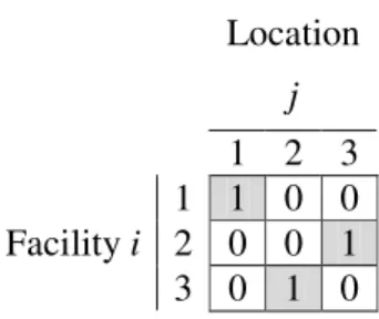
Recall that for any feasible solution to the QAP, the decision variables form a permutation matrix each corresponding to a one-to-one onto assignment of facilities to locations. In Figure 2, a small example for n = 3 is depicted, where the entry (i,j) of the matrix denotes the value of the assignment variable xij. The

Assignment Matrix in the example represents the solution where facility 1 is assigned to location 1 (x11 = 1), facility 2 is assigned to location 3 (x23 = 1), and

(25)

Location j 1 2 3 1 1 0 0 Facility i 2 0 0 1 3 0 1 0

Figure 2: An Example of Assignment Matrix

Perhaps more important than the Assignment Matrix is the Pairwise Assignment Matrix that represents the values of the quadratic terms xijxkl.

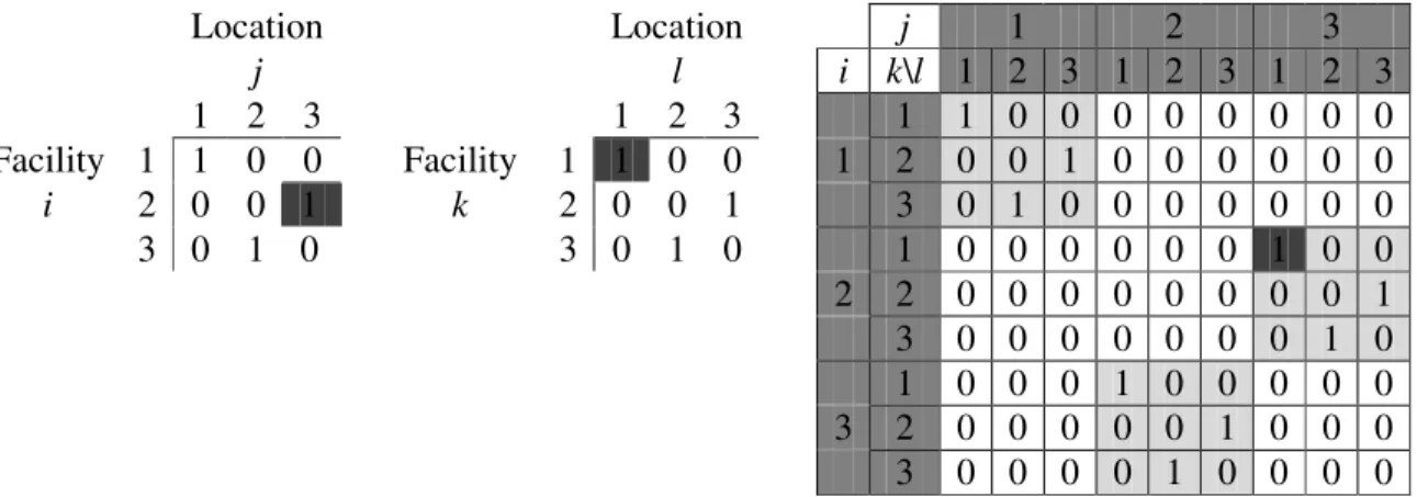
Although the assignment variables represent the core decisions, the costs are incurred by pairs of assignment variables. It is not an easy task to represent these n4 values in two dimensions in a structured way. Hahn et al. (1998) use the scheme depicted in Figure 3 that enables us to better understand the structure of the pairwise interactions of assignment decisions. The rows of the Pairwise Assignment Matrix are labeled with facility pairs (i,k) and the columns are labeled with location pairs (j,l). The entry in row (i,k) and column (j,l) of the Pairwise Assignment Matrix is the value of the quadratic term xijxkl. In Figure 3,

the row (and column) labels are 11, 12, 13, 21, 22, 23, 31, 32, and 33 where the leading index is shown as a header in the leftmost column and the topmost row. Observe that whenever the ij-entry is 1 in the assignment matrix (of Figure 2), a copy of the assignment matrix is reproduced in the Pairwise Assignment Matrix (of Figure 3) in the submatrix corresponding to the header indices i and j. Observe also that whenever xij = 0 in the Assignment Matrix, all the entries in the

submatrix corresponding to header indices i and j are also zero. We note that this matrix is the result of the Kroenecker product of an assignment / permutation matrix X with itself. Simply put, if we denote the Assignment Matrix as X, then submatrix (i,j) of the Pairwise Assignment Matrix is equal to xijX. The objective

function value for a given solution is returned by the sum of the cost coefficients corresponding to the 1’s in the Pairwise Assignment Matrix (Cijkl for the entry in

(26)

j 1 2 3 i k\l 1 2 3 1 2 3 1 2 3 Location pairs 1 1 0 0 0 0 0 0 0 0 2 0 0 1 0 0 0 0 0 0 1 3 0 1 0 0 0 0 0 0 0 1 0 0 0 0 0 0 1 0 0 2 0 0 0 0 0 0 0 0 1 2 3 0 0 0 0 0 0 0 1 0 1 0 0 0 1 0 0 0 0 0 2 0 0 0 0 0 1 0 0 0 3 3 0 0 0 0 1 0 0 0 0 Facility pairs

Figure 3: Pairwise Assignment Matrix and its Submatrices

These two matrices play a crucial role in our forthcoming analysis. In the next section, we will demonstrate that the auxiliary variables of the linearizations available in the literature correspond to simultaneous effects of decisions in two subsets of the Assignment Matrix. As a consequence, the auxiliary variables represent the cost incurred by certain subsets of the Pairwise Assignment Matrix. Each such subset corresponds to a subset sum of the quadratic objective function

∑

= n l k j i kl ij ijklx x C 1 , , ,

. In brief, we will be using the Assignment Matrix, the Pairwise Assignment Matrix, and the quadratic objective function to analyze the patterns of the models in the literature.

2. 2 Analysis of the Formulations in the Literature

As stated in Chapter 1, linear MIP models for the QAP are customarily referred to as linearizations. The QAP is originally stated as a nonlinear problem

(27)

while any attempt to describe it by linear inequalities and a linear objective function transforms it to a linear MIP. To be able to linearize the QAP, we need to define auxiliary variables that describe the cost contribution of the quadratic interactions. Thus, the core structure of the linearization process is shaped by the way that the auxiliary variables are defined. Generally, each type of auxiliary variable describes the total cost of the simultaneous effects of decisions in some two subsets of the Assignment Matrix. The models we are about to analyze differ in the level of aggregation of these costs.

We now proceed to demonstrate our foregoing observation on the models in the literature. Even though many different linearization techniques have been proposed for various special cases (Love and Wong, 1976; Christofides and Benavent, 1989), models based on Lawler’s pairwise assignment variables have dominated the literature. The author defined the variables yijkl = xijxkl so as to

represent the simultaneous effect of every pair of the assignment decisions.

Later, many other authors used this variable definition to construct linearizations of the QAP (Frieze and Yadegar, 1983; Resende, Ramakrishnan, and Drezner, 1994; Adams and Johnson, 1994). One of these studies by Adams and Johnson (1994) includes a proof of the fact that their linearization is at least as strong as the well-known GLB. The authors also show that many lower bound generation methods may be perceived as Lagrangean relaxations of their formulation. The formulation by Adams and Johnson (1994), which is known to yield the strongest lower bound among the formulations with O(n4) variables, follows: (IP1)

∑

= n l k j i ijkl ijkly C 1 , , , min (14)

(28)

s.t. n i x n j ij 1 1,..., 1 = ∀ =

∑

= (15) n j x n i ij 1 1,..., 1 = ∀ =

∑

= (16) n l j i x y _ij n k ijkl , , 1,..., 1 = ∀ =

∑

= (17) n k j i x y _ij n l ijkl , , 1,..., 1 = ∀ =

∑

= (18) n l k j x y _kl n i ijkl , , 1,..., 1 = ∀ =

∑

= (19) n l k i x y _kl n j ijkl , , 1,..., 1 = ∀ =

∑

= (20) l j k i n l k j i y y_ijkl = _klij ∀, , , =1,..., : < , ≠ (21)

{ }

i j n x_ij ∈ 0,1 ∀, =1,..., (22)

{ }

i j k l n y_ijkl ∈ 0,1 ∀, , , =1,..., (23)

Lawler’s linearization with auxiliary variables yijkl accounts for the

simultaneous effect of the pair of assignment variables xij and xkl. The pairs of

subsets of the Assignment Matrix under consideration are the pairs of assignment variables. Any such pair corresponds to a single cell of the Pairwise Assignment Matrix, as depicted in Figure 4.

(29)

Location Location j 1 2 3 j l i k\l 1 2 3 1 2 3 1 2 3 1 2 3 1 2 3 1 1 0 0 0 0 0 0 0 0 Facility 1 1 0 0 Facility 1 1 0 0 1 2 0 0 1 0 0 0 0 0 0 i 2 0 0 1 k 2 0 0 1 3 0 1 0 0 0 0 0 0 0 3 0 1 0 3 0 1 0 1 0 0 0 0 0 0 1 0 0 2 2 0 0 0 0 0 0 0 0 1 3 0 0 0 0 0 0 0 1 0 1 0 0 0 1 0 0 0 0 0 3 2 0 0 0 0 0 1 0 0 0 3 0 0 0 0 1 0 0 0 0

Figure 4: Lawler’s Linearization

Kaufman and Broeckx (1978) defined the variables =

∑

l k kl ijkl ij ij x C x w , to represent by wij the contribution of each assignment variable xij to the overall

cost. This linearization is somehow less favored in the literature, due to its weaker lower bound. Observe that, in terms of our tools of analysis, the relevant subsets of the Assignment Matrix under consideration are the pairings of each assignment variable with the overall Assignment Matrix. Hence, the variable wij

stands for the simultaneous effect of the assignment variable xij with the rest of

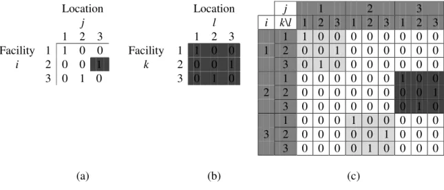
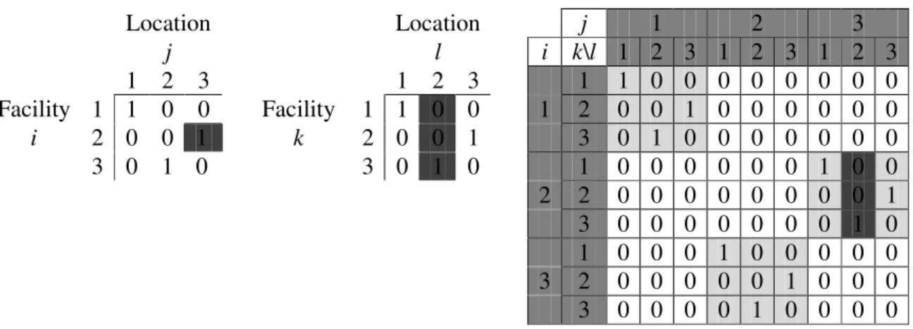
the Assignment Matrix. Figure 5 illustrates such a pairing corresponding to ij = 23 in 5(a) with the entire Assignment Matrix in 5(b). The resulting submatrix in the Pairwise Assignment Matrix corresponding to header indices 2,3 is marked in 5(c). The cost contribution that results from this interaction is the sum of the cost elements that correspond to the 1’s in the darkest colored submatrix of Figure 5(c). The formulation by Kaufman and Broeckx follows:

(IP2)

∑

= n j i ij w 1 , min (24)

(30)

s.t. n j i x M x C w n l k ij kl ijkl ij (1 ) , 1,..., 1 , = ∀ − − ≥

∑

= (25) n j i w_ij ≥0 ∀, =1,..., (26) and (15), (16), (22)

where M is a sufficiently large constant. Location Location j 1 2 3 j l i k\l 1 2 3 1 2 3 1 2 3 1 2 3 1 2 3 1 1 0 0 0 0 0 0 0 0 Facility 1 1 0 0 Facility 1 1 0 0 1 2 0 0 1 0 0 0 0 0 0 i 2 0 0 1 k 2 0 0 1 3 0 1 0 0 0 0 0 0 0 3 0 1 0 3 0 1 0 1 0 0 0 0 0 0 1 0 0 2 2 0 0 0 0 0 0 0 0 1 3 0 0 0 0 0 0 0 1 0 1 0 0 0 1 0 0 0 0 0 3 2 0 0 0 0 0 1 0 0 0 3 0 0 0 0 1 0 0 0 0 (a) (b) (c)

Figure 5: Kaufman and Broeckx’s Linearization

An even less favored formulation is that of Balas and Mazzola (1980), for which they define a single auxiliary variable, =

∑

l k j i kl ij ijklx x C w , , , , to represent the overall cost. (IP3) w min (27)

(31)

n kl x l k x l k j i kl ij ijklx x Mx x QAP C w kl kl ∈ ∀ − ≥

∑

= ∀ = ∀ * 0 : , 1 : , , , * * * (28) 0 ≥ w (29) and (15), (16), (22)

where QAPn_{denotes the set of all feasible solutions for a QAP of size n.}

Constraint set (28) forces the single auxiliary variable to be greater than or equal to the objective function value yielded by x*, if x = x*

, and has no effect otherwise. In this case, the authors define a single variable that pairs up the Assignment Matrix with itself. Figure 6(a)(b) identify the submatrices corresponding to the auxiliary variable w while the interaction of these submatrices yields the entire Pairwise Assignment Matrix shown in 6(c).

Location Location j 1 2 3 j l i k\l 1 2 3 1 2 3 1 2 3 1 2 3 1 2 3 1 1 0 0 0 0 0 0 0 0 Facility 1 1 0 0 Facility 1 1 0 0 1 2 0 0 1 0 0 0 0 0 0 i 2 0 0 1 k 2 0 0 1 3 0 1 0 0 0 0 0 0 0 3 0 1 0 3 0 1 0 1 0 0 0 0 0 0 1 0 0 2 2 0 0 0 0 0 0 0 0 1 3 0 0 0 0 0 0 0 1 0 1 0 0 0 1 0 0 0 0 0 3 2 0 0 0 0 0 1 0 0 0 3 0 0 0 0 1 0 0 0 0 (a) (b) (c)

Figure 6: Balas and Mazzola’s Linearization

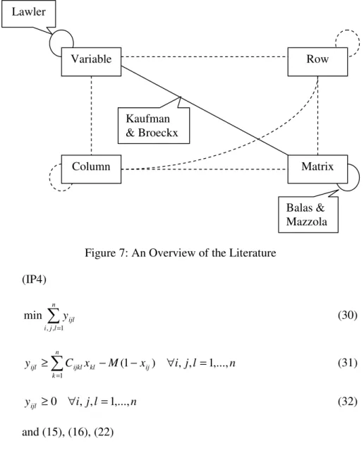
From our observations up to this point, we can see that any possible partitioning of the Pairwise Assignment Matrix into any two subsets would result in a different linearization. An auxiliary variable is introduced by each such

(32)

pairing. In order to better model the QAP, we feel the need to identify certain patterns in the foregoing formulations. We can easily observe that there are two types of subsets of the Assignment Matrix that have been used in the literature in the modeling process. One type is a single entry of the Assignment Matrix (i.e. single assignment variables) and the other type is the whole Assignment Matrix. Pairings of type I or type II with type I or type II yield the linearizations of Lawler, of Kaufman and Broeckx, and of Balas and Mazzola. Even though not seen in the literature (except Erdoğan and Tansel, 2005), the columns and the rows of the Assignment Matrix are also eligible to be used for constructing linearizations. The four types of subsets (single entry, column, row, and the whole Assignment Matrix) seem to yield the best physical interpretations for the corresponding cost aggregations. So, we base our analysis on these subsets. The graph in Figure 7 depicts the current situation of the literature. Each subset is denoted as a node and the arcs (solid lines) denote the interactions analyzed in the literature. The arcs depicted by broken lines in the figure are linearizations that have not yet been analyzed in the literature except for the linearizations introduced in a recent work of ours (Erdoğan and Tansel, 2005). We want to emphasize that each arc implies a unidirectional relation. For example, one can define the variables of Kaufman and Broeckx as the interaction of the Assignment Matrix and a single assignment variable ( =

∑

j i ij ijkl kl kl x C x w , ) and still construct the same formulation. In the next section, we focus on the interactions corresponding to broken lines and present the resulting new formulations for the QAP.

2. 3 New Formulations

To complete the picture in Figure 7, let us start with the interaction between a variable and a column. The corresponding submatrix in the Pairwise Assignment Matrix is a column of the submatrix corresponding to the assignment variable, as

(33)

depicted in Figure 8. Following the examples above, we define the variable

∑

= = n k kl ijkl ij ijl x C x y 1

. This nonlinear representation shows that the variable

yijl represents the interaction between the assignment variable xij and the l’th

column of the Assignment Matrix. Using this variable definition, the following formulation is constructed:

Figure 7: An Overview of the Literature (IP4)

∑

= n l j i ijl y 1 , , min (30) n l j i x M x C y _ij n k kl ijkl ijl (1 ) , , 1,..., 1 = ∀ − − ≥

∑

= (31) n l j i y_ijl ≥0 ∀, , =1,..., (32) and (15), (16), (22) Variable Row Column Matrix Lawler Balas & Mazzola Kaufman & Broeckx

(34)

where M is a large constant. Observe that constraint (31) forces the variable y_ijl

to be greater than or equal to

∑

= n k kl ijklx C 1

wheneverx_ij =1, and has no effect otherwise. Location Location j 1 2 3 j l i k\l 1 2 3 1 2 3 1 2 3 1 2 3 1 2 3 1 1 0 0 0 0 0 0 0 0 Facility 1 1 0 0 Facility 1 1 0 0 1 2 0 0 1 0 0 0 0 0 0 i 2 0 0 1 k 2 0 0 1 3 0 1 0 0 0 0 0 0 0 3 0 1 0 3 0 1 0 1 0 0 0 0 0 0 1 0 0 2 2 0 0 0 0 0 0 0 0 1 3 0 0 0 0 0 0 0 1 0 1 0 0 0 1 0 0 0 0 0 3 2 0 0 0 0 0 1 0 0 0 3 0 0 0 0 1 0 0 0 0

Figure 8: Multicommodity Flow Formulation

The way we construct constraint (31) will serve as an example for the formulations to follow in this section. Whenever one of the subsets is a single assignment variable, the simultaneous effect of the subsets is linearized as soon as the variable is decided. For this case,

∑

= = n k kl ijkl ijl C x y 1 ifx_ij =1, and y_ijl =0

ifx_ij =0. Hence, we have constructed constraint (31) by enumeration on possible

values xij can take, i.e. to force a lower bound of

∑

= n k kl ijklx C 1 on y_ijl whenever 1 = ij

x , and to have no effect whenever x_ij =0. The same constraint construction method may be used if one of the subsets is a column or a row, by enumeration on the possible assignments in the column or row. For example the linearization above can be recast as:

(35)

n l k j i x M x C y_ijl ≥ _ijkl _ij − (1− _kl) ∀, , , =1,..., (33)

Notice that constraint set (33) is constructed by enumeration on the decisions in column l, i.e. for each possible decision xkl. It forces a lower bound

of C_ijklx_ij on y_ijl whenever x_kl =1, and has no effect whenever x_kl =0.

Although this formulation is quite similar to the formulation of Kaufman and Broeckx, this modeling paradigm gives us a structure to exploit for the Koopmans-Beckmann form. For the Koopmans-Beckmann form, the variable

definition becomes

∑

= = n k kl jl ik ij ijl x f d x y 1

which can further be simplified to

∑

= = n k kl ik ij ijl x f x y 1 '

, with the term djl becoming the objective function coefficient

of '

ijl

y . The variable '

ijl

y also has a physical meaning: it represents the total material flow from location j to location l whenever facility i is located at j. This flow based interpretation suggests adding flow conservation constraints into the formulation: (IP4’)

∑

= n l j i ijl jly d 1 , , ' min (34) s.t. n j i f x y n l n k ik ij ijl , , 1,..., 1 1 ' = ∀       =

∑

= = (35) n l i x f y n j kl n k ik ijl , , 1,..., 1 1 ' = ∀ =

∑

= = (36)

(36)

n l j i x M x f y _ij n k kl ik ijl (1 ) , , 1,..., 1 ' = ∀ − − ≥

∑

= (37) n l j i y_ijl' 0, , , 1,..., = ∀ ≥ (38) and (15), (16), (22)

We now prove the validity of IP4’.

Theorem 1: Let x be a feasible solution to an instance of the QAP defined by matrices F and D with objective value zQAP(x). Then, there exists a unique vector

'

y such that (x, '

y ) is feasible to IP4’ with objective value zIP4’(x,y') = zQAP(x).

Proof: With x being feasible to the QAP, constraints (15), (16), and (22) are satisfied. For each i ∈ {1,…,n}, let a(i) be the location index j for which xij = 1.

Similarly, for each location j, let a-1(j) be the facility index i for which xij = 1.

Since xij = 0 ∀ j ≠ a(i), (35) and (38) imply that yijl' =0 ∀ j ≠ a(i) and i ∈

{1,…,n}. Consequently, the left side of (36) gives ' ) ( li ia

y (because all terms except for j = a(i) are zero), while the right side of (36) gives f_ia−1₍_l₎(because all

terms except for l = a-1(j) are zero). Hence, '

y is uniquely determined by the equations } ,..., 1 { , ) ( ' ) ( f 1 i l n y_ia_i_l = _ia− _l∀ ∈ (39) and ' ijl y = 0 ∀ j ≠ a(i) and i, l ∈ {1,…,n} (40) Solution '

y constructed in this way satisfies (38). It also satisfies (36) by construction. The only remaining possibility to be checked is constraint (35). If j ≠ a(i), then (35) gives zero on both sides. If j = a(i), the left side of (35) is

(37)

∑

= n l l i ia y 1 ' )

( while the right side is

∑

= n k ik f 1 . Since ' ₍₎ ) (_i_l _ia1 _l ia f y = − by construction, the left side is

∑

= − n l l ia f 1 ()

1 , which is the same as

∑

= n k ik f 1

. This proves the uniqueness

and feasibility of (x, '

y ) to IP4’ for each feasible x to QAP.

To prove zIP4’(x,y) = zQAP(x), observe that fikdjlxijxkl = 0, unless i = a

-1_{(j) and}

k = a-1(l), in which case it is f_a−1₍_j₎_a−1₍_l₎d_jl. Since the objective value of IP4’ gives

∑

= − − n l j a ja l jlf d 1 , ( ) () 1 1 , it is the same as

∑

= n l k j i kl ij jl ikd x x f 1 , , , . □

IP4 and IP4’ has O(n3

) variables and O(n3

) constraints. Both formulations are valid for arbitrary distance data. Notice that the proof of Theorem 1 does not involve the constraint set (37). This formulation will be referred as the Multicommodity Flow Formulation for the rest of this study. Next, we focus on the interaction between a variable and a row. The corresponding reflection on the Pairwise Assignment Matrix is a row of the submatrix corresponding to the assignment variable, as depicted in Figure 9.

Following the examples above, we define the variable

∑

= = n l kl ijkl ij ijk x C x t 1 . This representation shows that the variable tijk represents the interaction between

the assignment variable xij and k’th row of the Assignment Matrix. Using this

variable definition, a formulation conjugate to IP4 may be constructed. Similarly, the extension of this formulation to the Koopmans-Beckmann form results in variables representing the induced distance between two facilities (and another formulation conjugate to IP4’). Although the word “commodity” does not make sense when we speak of distances, since this formulation is the conjugate of the

(38)

Multicommodity Flow Formulation presented above, it will be referred to as the Multicommodity Distance Formulation in the rest of this study. We omit these formulations for the sake of brevity.

Figure 9: Multicommodity Distance Formulation

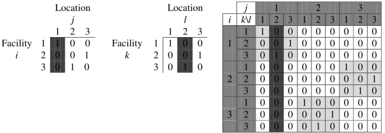
Next we focus on the interactions of columns of the Assignment Matrix. As depicted in Figure 10, the reflection of this interaction is a column of the Pairwise Assignment Matrix.

(39)

We define the corresponding variable as =

∑

k i kl ij ijkl jl C x x y , . The variable yjl

represents the interaction between the j’th and l’th columns of the Assignment Matrix. The resulting formulation follows:

(IP5)

∑

= n l j jl y 1 , min (41) s.t. n l j i x M x C y _ij n k kl ijkl jl (1 ) , , 1,..., 1 = ∀ − − ≥

∑

= (42) n l j y_jl ≥0,∀ , =1,..., (43) and (15), (16), (22)

Constraint (42) forces the variable yjl to be greater than or equal to

∑

= n k kl ijklx C 1

wheneverx_ij =1, and has no effect otherwise. As in the case of (IP4), this modeling paradigm allows us to move towards a more specific formulation for the Koopmans-Beckmann form. For this form, the variable definition

becomes

∑

= = n k i kl ij jl ik jl f d x x y 1 ,

which can be further simplified to

∑

= = n k i kl ij ik jl f x x y 1 , '

where the term djl becomes the objective function coefficient

of the variable '

jl

y . This variable definition also has a physical meaning: it defines (gives) the total material flow from location j to location l. This gives us the opportunity to add flow conservation constraints to the formulation:

(40)

(IP5’)

∑

= n l j jl jly d 1 , ' min (44) s.t. n j x f y n l n i ij n k ik jl , 1,..., 1 1 1 ' = ∀       =

∑

∑ ∑

= = = (45) n l x f y n j n k kl n i ik jl , 1,..., 1 1 1 ' = ∀       =

∑

∑ ∑

= = = (46) n l j i x M x f y _ij n k kl ik jl (1 ) , , 1,..., 1 ' = ∀ − − ≥

∑

= (47) n l j y'_jl ≥0,∀ , =1,..., (48) and (15), (16), (22)

Constraint (47) forces the variable '

jl

y to be greater than or equal to

∑

= n k kl ikx f 1

whenever x_ij =1, and has no effect otherwise. We now prove the validity of the formulation.

Theorem 2: Let x be a feasible solution to an instance of the QAP. Then, there exists a unique '

y such that (x,y') is feasible to IP5’ with objective function

value ( , ') ( )

'

5 x y z x

z_IP = _QAP .

Proof: With x being feasible to the QAP, constraints (15), (16), and (22) are satisfied. With a-1(j) denoting the facility index i for which xij = 1, (45) and (46)

give, respectively, that

∑

= = − = n l n k a jk jl f y 1 1 ( ) ' 1 and

∑

= = − = n j n i ia l jl f y 1 1 () ' 1 . Constraint

(41)

(47) sets the exact lower bound of each flow as '

il

y ≥ f_a−1₍_j₎_a−1₍_l₎. This upper

bound must be satisfied as equality, otherwise constraints (45) and (46) are violated. This proves the uniqueness and feasibility of (x, '

y ) to IP5’ for each feasible x to QAP.

To prove zIP5’(x,y) = zQAP(x), observe that y = il' f_a−1(_j)_a−1(_l), implying that the

objective value of IP5’ is

∑

= − − n l j a ja l jl f d 1 , ( ) () 1

1 which is the same as

∑

= n l k j i kl ij jl ikd x x f 1 , , , .□

This formulation will be referred to as the Single Commodity Flow Formulation in the rest of this study. IP5 and IP5’ has O(n2) variables and O(n3) constraints. Note that both formulations are valid for arbitrary distance data. Unlike the Multicommodity Flow Formulation, the flow conservation constraints are not sufficient to define the set of feasible solutions. As stated in the proof, '

il y = 1₍ ₎ 1₍₎ l a j a

f − − for every permutation a, which implies that variables

'

y take permuted values of the flow matrix. This provides an opportunity to exploit any structure that may be available in the flow matrix.

We next focus on the interactions between the rows of the Assignment Matrix. In this case, the induced subset is a row of the Pairwise Assignment Matrix, as depicted in Figure 11.

(42)

Figure 11: Single Commodity Distance Formulation

Following the scheme above, we define the variable

∑

= = n l j kl ij ijkl ik C x x t 1 , . The variable tik represents the interaction between the i’th and k’th rows of the

Assignment Matrix. Using this variable definition, a formulation conjugate to IP5 may be constructed. Similar to the Multicommodity Flow Formulation case, the extension of this formulation to the Koopmans-Beckmann form results in variables representing the induced distance between two facilities (and another formulation conjugate to IP5’). Hence, these formulations will be referred to as the Single Commodity Distance Formulation in the rest of this study. We omit this formulation as it is straightforward to derive it.

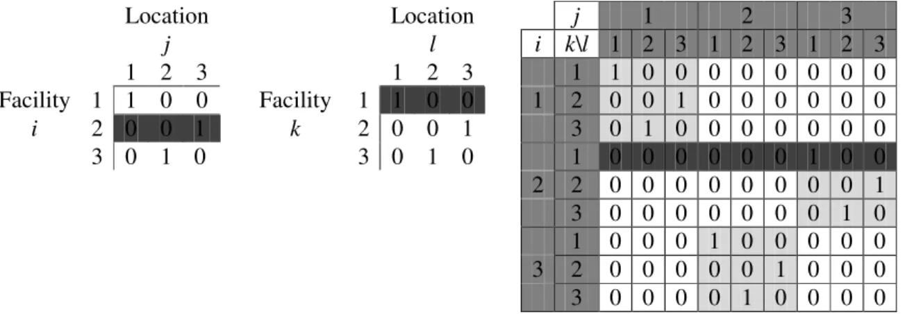
We now focus on the interactions between the row of the Assignment Matrix and the whole Assignment Matrix. In this case, the induced submatrix in the Pairwise Assignment Matrix is a submatrix consisting of all rows associated with the header index of the chosen row in the Assignment Matrix (depicted in Figure 12).

(43)

Figure 12: Facility-Based Formulation

For this case, we define the variable

∑

= = n l k j kl ij ijkl i C x x w 1 , , . The variable wi

represents the interaction between the i’th row of the Assignment Matrix the whole Assignment Matrix. Using this variable definition, the following formulation may be constructed:

(IP6)

∑

= n i i w 1 min (49) n j i x M x C w _ij n l k kl ijkl i (1 ) , 1,..., 1 , = ∀ − − ≥

∑

= (50) n i w_i ≥0 ∀ =1,..., (51) and (15), (16), (22)