Prototypes : exemplar based video representation

PROTOTYPES: EXEMPLAR BASED VIDEO

REPRESENTATION

a thesis submitted to

the graduate school of engineering and science

of bilkent university

in partial fulfillment of the requirements for

the degree of

master of science

in

computer engineering

By

¨

Ozge Yal¸cınkaya

June 2016

PROTOTYPES: EXEMPLAR BASED VIDEO REPRESENTATION By ¨Ozge Yal¸cınkaya

June 2016

We certify that we have read this thesis and that in our opinion it is fully adequate, in scope and in quality, as a thesis for the degree of Master of Science.

Selim Aksoy(Advisor)

¨

Oznur Ta¸stan

Sinan Kalkan

Approved for the Graduate School of Engineering and Science:

Levent Onural

ABSTRACT

PROTOTYPES: EXEMPLAR BASED VIDEO

REPRESENTATION

¨

Ozge Yal¸cınkaya

M.S. in Computer Engineering Advisor: Selim Aksoy

June 2016

Recognition of actions from videos is a widely studied problem and there have been many solutions introduced over the years. Labeling of the training data that is required for classification has been an important bottleneck for scalability of these methods. On the other hand, utilization of large number of weakly-labeled web data continues to be a challenge due to the noisy content of the videos. In this study, we tackle the problem of eliminating irrelevant videos through pruning the collection and discovering the most representative elements.

Motivated by the success of methods that discover the discriminative parts for image classification, we propose a novel video representation method that is based on selected distinctive exemplars. We call these discriminative exemplars as “pro-totypes” which are chosen from each action class separately to be representative for the class of interest. Then, we use these prototypes to describe the entire dataset. Following the traditional supervised classification methods and utilizing the available state-of-the-art low and deep-level features, we show that even with simple selection and representation methods, use of prototypes can increase the recognition performance. Moreover, by reducing the training data to the selected prototypes only, we show that less number of carefully selected examples could achieve the performance of a larger training data. In addition to prototypes, we explore the e↵ect of irrelevant data elimination in action recognition and give the experimental results which are comparable to or better than the state-of-the-art studies on benchmark video datasets UCF-101 and ActivityNet.

Keywords: action recognition, weakly-labeled data, discriminative exemplars, video representation, iterative noisy data elimination, feature learning.

¨

OZET

PROTOT˙IPLER: ¨

ORNEK TABANLI V˙IDEO TEMS˙IL˙I

¨

Ozge Yal¸cınkaya

Bilgisayar M¨uhendisli˘gi, Y¨uksek Lisans Tez Danı¸smanı: Selim Aksoy

Haziran 2016

Videolardan hareketlerin tanımlanması yaygın olarak ¸calı¸sılan bir problemdir ve yıllar boyunca ¨onerilen bir¸cok ¸c¨oz¨um olmu¸stur. Sınıflandırma i¸cin gerekli olan e˘gitim verisini etiketleme, bu y¨ontemlerin ¨ol¸ceklenebilirli˘gi i¸cin ¨onemli bir sorun olmu¸stur. Di˘ger taraftan, videoların g¨ur¨ult¨ul¨u i¸ceri˘gi nedeniyle ¸cok sayıdaki zayıf etiketli web verilerinin kullanımı bir sorun olmaya devam etmektedir. Bu ¸calı¸smada, koleksiyonu budama yoluyla ilgisiz videoların elenmesi ve en temsilci elemanların ke¸sfedilmesi problemlerini ele almaktayız.

G¨or¨unt¨u sınıflandırma i¸cin ayrı¸stırıcı par¸caları ke¸sfeden y¨ontemlerin ba¸sarısın-dan esinlenerek, se¸cilen ayırt edici ¨ornekleri temel alan yeni bir y¨ontem ¨oneriyoruz. Her hareket sınıfından o sınıf i¸cin tanımlayıcı olacak ¸sekilde ayrı ayrı se¸cilen bu ayrı¸stırıcı ¨orneklere “prototipler” demekteyiz. Sonrasında, bu prototip-leri t¨um veri k¨umesini betimlemede kullanmaktayız. Geleneksel sınıflandırma y¨ontemlerini izleyerek ve mevcut olan en g¨uncel alt ve derin d¨uzeydeki ¨oznitelikleri kullanarak, en basit se¸cim ve tanımlama y¨ontemleriyle bile, prototip kullanımının hareket tanıma performansını arttırabilece˘gini g¨osteriyoruz. Ayrıca, e˘gitme verilerinin sadece se¸cilmi¸s prototiplere azaltılmasıyla, daha az sayıdaki dikka-tle se¸cilmi¸s ¨orneklerin, daha b¨uy¨uk sayıdaki e˘gitme verilerinin performansına ula¸sabilece˘gini g¨osteriyoruz. Prototiplere ek olarak, hareket tanımlamada ilgi-siz veri elemesinin etkisini ara¸stırıyoruz ve en g¨uncel ¸calı¸smalardan daha iyi veya kıyaslanabilir olan deneysel sonu¸cları, kriter olarak g¨or¨ulen UCF-101 ve Activi-tyNet video veri k¨umeleri ¨uzerinden veriyoruz.

Anahtar s¨ozc¨ukler : hareket tanımlama, zayıf etiketlenmi¸s veri, ayırt edici ¨ornekler, video tanımlama, yinelemeli g¨ur¨ult¨ul¨u veri eleme, ¨oznitelik ¨o˘grenimi.

Acknowledgement

First, I wish to express the deepest appreciation to Assoc. Prof. Pınar Duygulu S¸ahin for her guidance and persistent help through the learning process of this thesis. Also, I want to thank Assoc. Prof. Selim Aksoy for his advices throughout my graduate life.

I am grateful to my family Oya, Abdurrahman and Anıl Yal¸cınkaya for their constant support and moral throughout my life. None of these would have been possible without them.

I would like to thank my childhood friend C¸ a˘glar Tun¸c and his fiance ¨Oyk¨u Arkan, my cousins Gizem Orta and Arman Tekinalp, my dearest high school friends Ya˘gmur Karaku¸s, Buket S¸ahin, Melike Kara¸cam and Nihan ¨Oz¸celik for always being with me to motivate when I need.

And lastly, I would like to thank Orhun Mert S¸im¸sek for adding meaning to my life and the unconditional support that allows me to pursue my career.

This thesis is partially supported by TUBITAK project with grant no 112E174 and CHIST-ERA MUCKE project.

vi

Contents

2.2.1 Discriminative Patch Idea . . . 9

2.2.2 Association Through Model Evaluation (AME) . . . 9

3 Prototypes 12 3.1 Prototype Selection . . . 13

3.1.1 Random Selection . . . 14

3.1.2 Discriminative Selection . . . 14

CONTENTS viii

3.1.4 AME Selection . . . 15

3.2 Prototype Based Representation . . . 16

3.2.1 Euclidean Similarity Values . . . 16

3.2.2 Exemplar SVM Scores . . . 17 4 Experimental Setup 20 4.1 Datasets . . . 20 4.1.1 UCF-101 . . . 20 4.1.2 ActivityNet . . . 21 4.1.3 Sports-S . . . 21 4.1.4 UCF-S . . . 22 4.2 Video Representation . . . 22 4.2.1 Low-level . . . 23 4.2.2 Deep-level . . . 23 4.3 Evaluation . . . 24

5 Results and Discussion 25 5.1 Prototype Experiments . . . 25

5.2 Analysis of AME for Action Recognition . . . 31

CONTENTS ix

5.2.2 Comparisons and Results . . . 32

List of Figures

1.1 Examples from Sports-1M dataset’s basketball action class which are collected from YouTube. As it can be seen, there are real basketball action videos as well as the irrelevant ones which include a ceremony or an interviewer. . . 2

2.1 AME overview [1]. The irrelevant instances are purified through iterative model evolution. In each iteration, while M1 _separates

candidate category references from global negatives, M2 _separates

category references from other candidates. . . 11

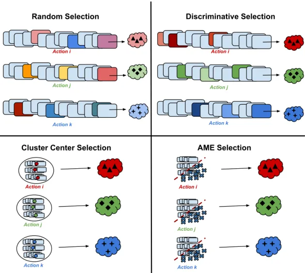
3.1 Illustration of prototype selection methods for three action classes. For random selection, we get less distinctive exemplars since we also choose irrelevant instances. Therefore, our prototypes can be considered weak. However, with discriminative selection [2] method, the selected samples are more representative for the class of interest. Likewise, cluster center selection gives a generalization of the data whereas AME [1] eliminates the noisy instances for more purified prototypes. . . 18

LIST OF FIGURES xi

3.2 An overview of prototype representation and used methods for three action classes. We represent each video in terms of selected prototypes. In order to do that, we use two di↵erent methods: (1) measuring the Euclidean distance between prototypes and a video, (2) calculating the SVM prediction scores of the video by using the models which are learned against a global negative set for each prototype. Then, we save the results in vectors for a proper description. . . 19

5.1 Classification results for di↵erent number of prototypes for both random and cluster center selection. As it can be seen from the graphics, the quality of the prototypes are more important than the amount of them. . . 36 5.2 Resulting exemplars of di↵erent selection methods for “basketball”

action class in Sports-S dataset. . . 37 5.3 Class based accuracy results for UCF-101 dataset with prototype

representation. The results are given for cluster center selection when k = 60 and Euclidean similarity representation. . . 38 5.4 E↵ects of AME [1] parameters on classification accuracy

both for UCF-101(left) and ActivityNet(right) datasets: (1) min elimination ratio which determines the rate of eliminated in-stances at the end of the iterations ; (2) M1 selection ratio specifies the positive to negative instances rate selected by M1 model; (3) M2 selection number indicates the number of instances that should be eliminated in each iteration. . . 39 5.5 Class based accuracies on ActivityNet classes after AME [1]

elim-ination. . . 40 5.6 Example of unsuccessful eliminated instances for ActivityNet class

LIST OF FIGURES xii

5.7 Example of successful eliminated instances by AME [1] for Activi-tyNet action classes. As seen from examples, AME is able to retain the representative instances while eliminating the irrelevant ones. The e↵ect of purifying the data is clearly seen on the performances (1) “Archery” class. Baseline: 31.57%, AME: 44.73%. (2) “Check-ing tires” class. Baseline: 26.82%, AME: 41.46%. (3) “Platform diving” class. Baseline: 56.66%, AME: 73.33%. . . 41

List of Tables

5.1 Results for UCF-S dataset. Baseline is: 48.72% . . . 27 5.2 Results for Sports-S dataset. Baseline is: 33.62% . . . 27 5.3 Class based accuracies on UCF-S and Sports-S for prototype

rep-resentation. . . 28 5.4 Prototypes as training data. . . 29 5.5 Prototype based representation results for UCF-101 and ActivityNet. 30 5.6 The best cluster numbers and the number of instances in per class

for each dataset. . . 31 5.7 UCF101 classification results after AME [1] elimination. In the

first column the state-of-the art results are given and second col-umn reports AME results over these baselines. . . 33 5.8 Comparison of AME [1] and Discriminative Patch method we

im-plemented based on the algorithm that is given in [2]. . . 33 5.9 Action recognition results on ActivityNet after AME [1]

elimina-tion. First column reports baseline classification results for deep level features and second column gives improvements of AME. . . 34

Chapter 1

Introduction

Searching for a video with the desired content is a challenging process due to the excessive amount of videos on the Internet that grow rapidly everyday. Every minute, 300 hours of videos are uploaded to YouTube alone1 _{and the videos}

watched everyday are at the level of hundreds of millions of hours2_{. In addition,}

according to statistics, there are over 120.000.000 videos in total on YouTube. The current methods have limitations to access the videos with a specific con-tent among this massive amount of data. Thus, a very large percentage of the videos lies almost inaccessible and plays an important role for the big visual data to be regarded as the “dark matter” of the Internet. Classification of the videos into predefined categories is the main attempt to solve this problem. However, despite the recent achievements for images, large scale video categorization con-tinues to be a challenge.

Manual annotation is required to have a clean training data for classification. However, labeling is a bottleneck not only due to the e↵ort required to annotate large amounts, but also due to the noisy nature of the videos. A single video may contain several parts some of which could be irrelevant. Therefore, a spe-cific category label may be inadequate to describe the full video. Moreover, the

1_{http://www.statisticbrain.com/youtube-statistics/} 2_{https://www.youtube.com/yt/press/statistics.html}

labeling procedure may be subjective and this can cause the data to be noisy and inconsistent.

The mass amount of data on the web itself has been a solution to handle the labeling e↵ort. However, using the weakly labeled data collected from the internet instead of a hand-crafted dataset brings several challenges. First of all, web data may have irrelevant tags. Secondly, one video can have multiple tags and determining which one is appropriate is difficult. Also, a single video may include many di↵erent actions or events even if the tag is relevant.

Figure 1.1: Examples from Sports-1M dataset’s basketball action class which are collected from YouTube. As it can be seen, there are real basketball action videos as well as the irrelevant ones which include a ceremony or an interviewer.

Therefore, the impurity of the weakly-labeled data is an important problem for learning models from these collections. Consider the sport videos collected through textual queries for a specific keyword. The collection may include the videos with real game scenes, as well as the audience, shows of the cheer girls, interviews with players, etc. that are all labeled with the same keyword (Fig-ure 1.1). If we use the entire collection as the training examples, the noise in the data may prevent to build good models since some of the training instances

does not include the desired action. Learning bad models cause us to be failed in prediction phase. Consequently, the e↵ect of spurious instances in the collection should be decreased before generating models for the categories since we need e↵ective models for accurate prediction. In order to do that, we focus on the description of the instances which are used in classification.

Representation of the videos through descriptors ranging from low-level fea-tures to semantic concepts has been a widely studied topic and with the recent advances on deep features, the importance of efficient and e↵ective representa-tions has been reconsidered again. Since the extracted descriptors do not consider the relevancy of the video, we focus on representing the data in a way that in-cludes the information of association to a specific concept. For this purpose, we explore the e↵ect of mid-level representations on the recognition performance by using the baseline representations.

Some of the instances of the training set tend to be visually distinctive and descriptive, and thus could be considered as representatives or exemplars to de-scribe the category. Moreover, some of the parts of the videos can be used as discriminative exemplars since videos of the same category are likely to include similar set of exemplars, some of which could also be individually shared within other videos. Based on these observations, we approach the problem as describ-ing the videos through representative short video clips or videos itself that we refer to as “prototypes”. The main idea of the prototypes is choosing only the descriptive instances from each class and then using them for representing the entire dataset in order to reduce the e↵ect of the noisy instances while learning the models. By this way, we measure the similarity of each instance to chosen distinctive prototypes which provides us a better representation than both low and deep-level descriptions.

We are inspired from the literature on finding the mid-level discriminative patches for specific image categories. These approaches follow the idea of finding patches that are distinctive among a large set of patches extracted from cate-gory images against large set of global negatives. Discovering meaningful mid-level components in videos have also been studied in the form of finding atomic

actions [3] in complex activities or descriptive spatio-temporal volumes for ac-tions [4]. However, the problem that we attack has important di↵erences from finding discriminative patches. First of all, we consider the videos as a whole, and therefore try to find the discriminative video examples, but not the parts of the videos. Furthermore, we require quite a few number of data examples compared to discriminative patch approaches that utilize large number of data.

Selecting the prototypes is an important problem since the entire representa-tion is based on them. Therefore, we investigate di↵erent methods for choosing appropriate exemplars and representing the data in terms of prototypes. We ex-periment on both low-level and deep-level features. For our research, we utilize ActivityNet, UCF-101 and a subset of Sports-1M benchmark video datasets.

In addition to prototype selection and representation methods, we also analyze the e↵ect of data pruning techniques. Specifically, we exploit Association Through Model Evolution(AME) which is proposed by Golge et al. [1] as a prototype selection method. We utilize AME for a better action recognition on weakly-labeled datasets since this method has a proven achievement on classification of weakly-labeled images.

In this study, we attack a more difficult problem and aim to discover discrimi-native examples to classify human activities in videos where intra-class di↵erences and inter-class similarities are larger. We experiment on UCF101 and ActivityNet datasets and report the results which are better than state-of-the-art. In addi-tion, we give the examination of AME parameters on classification results which is not explored in detail previously.

In the following, after reviewing the relevant studies in the broad literature of activity recognition and discriminative selection, the proposed method “proto-types” will be described with selection and representation methods. Experimen-tal results obtained on the datasets that we used will be presented followed by discussions.

Chapter 2

Background

In this chapter, we give the most recent methods that are used in action recog-nition in the literature by utilizing both low-level and deep-level features. After that, we explain the studies that are based on choosing discriminative instances for decreasing the e↵ect of the noise, which consist of the discriminative patch method and AME that we used in our work.

2.1

Action Recognition

Action recognition has been a widely studied topic and many approaches are proposed over the years [5]. The basic approaches for action representation can be extracting global spatio-temporal templates as in [6], using motion history images [7], space-time silhouettes of the actions [8], spatial motion descriptors like optical flows [9, 10] or utilizing still images’ parts and attributes for detecting the action [11] which can be specified as global descriptors. However, they were not able to handle the camera stabilization problems and appearance changes properly while tracking a moving object or doing segmentation. Therefore, local solutions have started to be used instead of the global ones.

More recently space-time local descriptors and trajectories are stated as ap-propriate representatives for action recognition. In addition, bag of visual words and fisher vector encoding methods are used for video-level representation. On the other hand, as an alternative to hand-crafted features, deep-level features learned by Convolutional Neural Networks have been recently adapted for video classification [12, 13, 14, 15, 16] and their success has been proven on benchmark datasets. In the following, we first describe the introduced methods based on the most recent low-level hand-crafted features. Then, we explore the current methods on deep-level features.

2.1.1

Low-level Representations

After obtaining successful results by using global representations and optical flow, local descriptors were introduced as novel low-level motion representations. Firstly, image descriptors have been generalized to video features such as 3D-SIFT [17], extended SURF [18] and HOG3D [19]. Laptev proposed Space Time Interest Points (STIP) by expanding the local interest points to spatio-temporal domain [20, 21, 22, 23, 24]. While extracting STIP features, they utilized Harris interest point detectors in order to locate the local structures. They detected the important variations both in space and time for a spatio-temporal local descrip-tor.

STIP features are encoded with the “bag of features” method in order to obtain a video level description which is pursued by a SVM classifier in several works [25, 26] that have proven to be successful. In these studies, they basically calculated the bag of spatio-temporal point representations of the videos after extracting STIP features. They managed to recognize realistic human actions in the movie clips which can be stated as challenging since they include diverse motions come from human nature.

After the achievements of spatio-temporal structures, dense trajectories were introduced by Wang et al. [27, 28]. In this work, they presented a novel trajectory description which is robust to irregular camera motions. They employed dense

points of each frame and track them according to optical flow vectors which give the motion information between frames. Moreover, they computed HOG ,HOF and MBH [29] descriptors along the trajectories to capture shape, appearance and motion information.

In addition to dense trajectories, Wang et al. proposed improved dense trajec-tories (IDT) as a more robust method to camera motions [30, 31] that outperform the other methods for recognition of complex activities with Fisher Vector encod-ing [32, 33].

2.1.2

Deep-level Representations

Deep features that are extracted from Convolutional Neural Networks (CNN) are proposed for image classification [34] and their performance has been proven to be successful recently. In the light of these achievements, many studies are intro-duced for action recognition with neural networks. Basically, videos are treated as image collections. Therefore, for each frame of a video a CNN representation is extracted. After that, a video-level prediction is calculated by fusing represen-tations of all frames.

Karpathy et al. proposed a network to learn motion information from raw images by using slow fusion [16] for large scale data. Simonyan et al. showed that using both single frame and optical flow images in two stream network provides a successful representation for videos [15] since optical flow is able to give temporal information whereas single frame gives spatial information.

In addition to utilizing 2D networks, several approaches employ 3D convolution in order to provide the temporal information as well [14, 13, 35]. Since using the temporal information while computing the video representation is more suitable for videos, using 3D CNN structures is more preferable.

Furthermore, a structure that utilizes depth map sequences [36], an end-to-end network that uses reinforcement learning to detect the most distinctive parts of

the videos for decreasing the data size [37], are introduced. Yue et al. proposed a pooling process as a convolutional layer for an accurate video level represen-tation [38]. They also employed Long Short-Term Memory (LSTM) networks for sequential learning from raw frames. Finally, Wang et al. presented a new video representation, trajectory-pooled deep-convolutional descriptor (TDD), by utilizing both hand-crafted and deep-level features.

2.2

Discriminative Selection

Similar to our work, there are many attempts to decrease the e↵ects of weakly-labeled data on classification. It has been shown that using the representative parts of the data may be a solution. Firstly, Singh et al. proposed discriminative patch approach for image classification [2] and it is used in many works [39, 40, 41, 42].

Jain et al. [43] proposed a method to detect discriminative parts of videos from spatio-temporal patches by using exemplar-SVM [44]. Chu et al. introduced a method for finding the subsequences that include similar visual content from temporal similarity [45]. Misra et al. [46] focused on discovering distinctive exemplars to cope with diversity in appearance for accurate object detection similar to our work. Golge et al. introduced a method for concept learning from noisy web images by clustering the data while detecting outliers [47] and an iterative approach named Association Through Model Evaluation (AME) to eliminate irrelevant data for better classification results [1]. A scene classification method is proposed in [48] by detecting the discriminative parts incrementally. In addition, CNNs are adapted for distinctive part detection while learning from weakly labeled data [49] and in an exemplar based manner [50].

In the following, we give the details of discriminative patch method and AME that we used in our work.

2.2.1

Discriminative Patch Idea

This method was introduced to discover representative and discriminative patches from images for a mid-level representation by Singh et al. [2]. Firstly, the authors extracted thousands of patches from the images in di↵erent scales and represent them by HOG features. Then, the algorithm created clusters for each class by using k-means. The most representative instances from each cluster were detected by selecting the top N instances that got the highest prediction score from SVM againts a global negative patch set. This process continued iteratively until the instances which got the highest scores did not change. As a result, the most distinctive cluster elements which were the furthest ones from negative set, were defined as discriminative and representative patches for the category classes.

In our work, we adopt this idea for videos and we consider each video as a patch in the given algorithm. Therefore, for each class, we use the most discriminative and representative instances instead of using the entire data. We employ this method for distinctive prototype selection.

2.2.2

Association Through Model Evaluation (AME)

AME is proposed to eliminate the noisy and irrelevant data from queried web images with an iterative model evaluation by linear classifiers [1]. In this method, a model is learned by utilizing positive class instances and a global negative set. After that, some of the category elements which are distant from the separating hyperplane are selected as confidently classified ones against global negatives and they are referred as possible positive class instances whereas the closer ones to the line are considered as spurious. Then, another model is learned for separating remaining positives and possible noisy elements for detecting intra-class variety.

The authors, combine the confidence scores of first and second models to mea-sure the instance saliency. The instances which have the lowest confidence scores are defined as the noisy ones and this procedure continues iteratively up to a

desired pruning level. In each iteration, remaining positive instances are used as the next training data.

Algorithm 1: AME

1 C₀ C 2 t 1

3 while stoppingConditionN otSatisf ied() do 4 M_t1 LogisticRegression(C_{t 1}, N ) 5 C_t+ selectT opP ositives(Ct 1, Mt1, p) 6 C_t Ct 1 Ct+ 7 M_t2 LogisticRegresstion(C_t+, C_t ) 8 [S₁, S₂ ] getConfidenceScores(C_t , M_t1M_t2) 9 It selectIrrelevantItems(Ct , S1, S2, r) 10 C_t C_{t 1} I_t 11 t t + 1 12 end 13 C Ct 14 return C

As depicted in Algorithm 1, C =_{c1, c2, . . . cm} refers to the videos in a class

and N = _{{n1, n2, ..., nl} refers to the vast numbers of global negatives. Each} vector is a d dimensional representation of a single video. At each iteration t, the first LR model M1 _{learns a hyper-plane between the candidate class instances}

C and global negatives N . Then, C is divided into two subsets: p instances in C that are farthest from the hyperplane are kept as the candidate positive set (C+_{) and the rest is considered as the negative set (C ) for the next model. C}+

is the set of salient instances representing the category references for the class and C is the set of possible spurious instances. The second LR model M2 _uses

C+ _{as positive and C as the negative set to learn the best possible hyperplane}

separating them. For each instance in C , by aggregating the confidence values of both models, r instances with the lowest scores are eliminated as irrelevant. This iterative procedure continues until it satisfies a stopping condition. They use M1 0_{s objective as the measure of data quality. As AME incrementally remove poor}

instances, it is expected to have better separation against the negatives.

We utilize this method to select the pure and representative prototypes by eliminating the irrelevant data. Moreover, we investigate the achievement of AME on action recognition by applying it to large-scale video benchmarks (Figure 2.1).

Videos Features 1 n M1 ... M1 M1 M1 M2 M2 Iterative Elimination

Figure 2.1: AME overview [1]. The irrelevant instances are purified through iter-ative model evolution. In each iteration, while M1 _{separates candidate category}

references from global negatives, M2 _{separates category references from other}

candidates.

We also examine the e↵ects of the parameter set and provide the analysis of video datasets.

AME has three parameters which a↵ect the elimination results. The maximum number of samples that must be eliminated is specified by min elimination ratio. For example, if this parameter is equal to 0.4, at least 40% of the instances should be eliminated from each class at the end of the iterations. M1 selection ratio determines the ratio of positive to negative samples that should be selected by M1

classifier which is the first model that is learned between positive and negative sets. The number of samples that should be eliminated in each iteration by learning the second model M2 _{is specified with M2 selection number .}

Chapter 3

Prototypes

We introduce a novel mid-level representation method for videos to be used in action recognition. Our main purpose is to reduce the adverse e↵ects of irrelevant and noisy instances on model learning for accurate action prediction.

We basically determine the discriminative instances which describe the data best and then we use them as the prototypes for representation of the entire data. We define prototypes as the videos or video clips being representatives for the entire collection.

The main idea is to replace the calculated features with a representation based on prototypes. Each clip is then replaced by a description based on the selected prototypes, with the length of the descriptor being the number of the prototypes. We select prototypes from all action classes in the training set. Complete steps of prototype based representation process can be seen in Algorithm 2.

Here, we select prototypes from each action class of training set, after deter-mining the amount of them. We use calculated baseline representations while choosing prototypes. Then, we compute the similarities between each prototype and instances from both training and test sets. As a result, new prototype based representations of all instances are calculated.

Algorithm 2: Prototype based representation

Data: T rainingSetbaseline, T estSetbaseline 1 prototypeN o N

2 foreach actionClass_i in T rainingSet_baseline do

3 prototypes[i] selectP rototypes(actionClass_i, prototypeN o) 4 end

5 foreach instance_i in T rainingSet_baseline do 6 foreach prototype_j in prototypes do

7 simV alues[j] calculateSimilarty(instancei, prototypej) 8 end

9 T rainingSet_proBasedRep[i] simV alues 10 end

11 foreach instancei in T estSetbaseline do 12 foreach prototypej in prototypes do

13 simV alues[j] calculateSimilarty(instance_i, prototype_j) 14 end

15 T estSet_proBasedRep[i] simV alues 16 end

17 return getP redictionScores(T rainingSet_proBasedRep, T estSet_proBasedRep)

We investigate di↵erent forms of prototype selection and prototype based rep-resentation. In the following, we give details of prototype selection methods. Then, the representation methods by the means of prototypes are explored.

3.1

Prototype Selection

Since describing the data with a noisy instance will cause failure in classification phase, using irrelevant and spurious data as prototype is not preferable. Bad exemplars will cause an inadequate representation for videos. Therefore, selecting the most representative prototypes is very essential for an accurate prototype based representation. Note that we select exemplars after we calculate the video level representations of the videos such as low-level or deep-level. Here, we give three di↵erent selection methods which are used in this work. An overview of the methods can be seen in Figure 3.1.

3.1.1

Random Selection

First of all, a possible prototype choice might be randomly picked exemplars from each class by ignoring distinctiveness. However, since there might be irrelevant data, selecting that inefficient exemplar will not provide the desired representa-tion. Nevertheless, our experiments show that even random selection provides better classification results due to decreased e↵ect of noise. It is because we rep-resent a noisy data in terms of prototypes which may include distinctive data as well. On the other hand, for a noisier dataset, random selection shows bad results compared to the hand-crafted dataset since the amount of spurious instances is higher.

3.1.2

Discriminative Selection

For discriminative selection, we directly used the algorithm that is given in [2]. Here, after generating clusters by k-means, the discriminative members of each cluster are selected by learning a SVM model for each instance. The instances that have top confidence scores against to the global negative set are taken as new cluster members. The process continues until cluster members are not changed. Consequently, at the end of the iterations, the resulting cluster members are indicated as the discriminative ones. For our experiment, we used each video in each class as a patch and we applied this algorithm to find the most distinctive videos or video clips.

3.1.3

K-Means Cluster Center Selection

As another prototype selection method, we employ k-means clustering. This time, we do not use the cluster instances but we choose k-means cluster centers as prototypes. The appropriate cluster number is chosen by the experiments.

instances that includes the representative information. Therefore, N number of cluster centers can provide a good distinctiveness for the class of interest and be used in representation of videos as prototypes.

3.1.4

AME Selection

Finally, we select prototypes by using AME [1] iterative elimination. Motivated by the success of irrelevant data elimination of AME, we choose the final purified set of current action class as discriminative instances. Since our intuition is not to use noisy data as prototypes, AME contributes for selection of more efficient exemplars in this study.

3.2

Prototype Based Representation

After selecting suitable exemplars, we describe all videos based on these pro-totypes instead of using low-level or deep-level representations. Hence, the new feature vector of video X from action class i can be regarded as Xf =

(p1

i, p2i, p3i, p1j, p2j, p3j, ..., pkz) where i, j, ..., z are the action classes and pki corresponds

to similarity value of a specific prototype from action class i with identity number k.

While calculating this representation, we utilize two di↵erent methods. An illustration of the methods can be seen in Figure 3.2.

3.2.1

Euclidean Similarity Values

One idea to calculate a prototype based representation is to look into the similar-ity between a set of prototypes and a video clip. In this representation method, we calculate the Euclidean distance between a video feature and selected proto-types in order to determine the similarity. Then, we create a new representation vector for the current video which includes the distance values to the prototypes. For instance, if we have N prototypes in total that are picked from each class, we will have N Euclidean distance values for one video. Hence, our new feature vector is formed by the computed distance values and have a dimension of 1_{⇥ N.} By doing that, we hold the information of which prototype is more similar to the video of interest. Likewise, new feature vector has the knowledge of which action the video belongs to. Thus, if the video is irrelevant or a noisy data, the distance measure between a representative prototype will be high so that its new feature vector values will be very di↵erent from those of a relevant video. This variety provides us a simple and accurate classification.

selected prototype as distinctive exemplar. The other values also give the in-formation of the action class that the video belongs to. On the contrary, if the elements of the new feature vector are close to 1, it is very possible that the video is an irrelevant instance.

Since noisy video’s new feature vector has di↵erent values from the others, it will have less e↵ect on model learning. We reduce the impact of the noisy instance while the di↵erence between relevant and irrelevant samples increases.

3.2.2

Exemplar SVM Scores

Another method to represent videos by the means of prototypes is using linear SVM confidence scores. For each selected prototype, we learn a model against a global negative dataset as in [44]. After obtaining the model structures, a prediction score is calculated for each video in the dataset by using learned hyper-planes for prototypes. Then, a new feature vector is formed from the prediction scores.

The new feature vector consists the information of classification results between prototypes and instances. According to distance to the learned model line, we can understand which clip is closer to global negatives and which one is relative to its action class. Similar to Euclidean distance affinity description, in the classification phase, this representation is useful in order to eliminate the adverse e↵ect of noisy instances.

Likewise, if there are N prototypes, we will have N SVM models and N pre-diction scores for each video in the dataset. After obtaining prepre-dictions, our new representation will be a feature vector of size 1_{⇥ N. Note that for all} represen-tation methods, we normalize the values into the range [0-1].

Random Selection Discriminative Selection

Cluster Center Selection AME Selection

Action i Action j Action k Action i Action j Action k Action i Action j Action k Action i Action j Action k

Figure 3.1: Illustration of prototype selection methods for three action classes. For random selection, we get less distinctive exemplars since we also choose irrele-vant instances. Therefore, our prototypes can be considered weak. However, with discriminative selection [2] method, the selected samples are more representative for the class of interest. Likewise, cluster center selection gives a generalization of the data whereas AME [1] eliminates the noisy instances for more purified prototypes.

Action i

Action j

Action k

Video clips

Prototypes

Prototype based

representation

Euclidean Similarity

Exemplar SVM Score

Figure 3.2: An overview of prototype representation and used methods for three action classes. We represent each video in terms of selected prototypes. In order to do that, we use two di↵erent methods: (1) measuring the Euclidean distance between prototypes and a video, (2) calculating the SVM prediction scores of the video by using the models which are learned against a global negative set for each prototype. Then, we save the results in vectors for a proper description.

Chapter 4

Experimental Setup

In this chapter, we provide the details of our experiments on the proposed meth-ods. First, we briefly explain the used benchmark datasets and then explore the video representations that we utilize for our baseline. Finally, the evaluation method of the classification results is demonstrated.

4.1

Datasets

4.1.1

UCF-101

The UCF-101 [51] contains 13,320 videos with 101 action classes including a set of activities such as human-object interactions, body motions, musical instruments and sports. Each category is organized into 25 groups, where each group consists of 4-7 clips of an action. It is reported that the videos from the same group share common features as similar background or viewpoint. There are 150 video clips in per class approximately and each video is stated as challenging due to the camera motion, viewpoint variations or illumination conditions. UCF-101 can be regarded as a hand-crafted dataset since the videos are trimmed.

In our experiments, we use given train/test splits for the evaluation of the baseline results. For all representation methods, we use the entire video frames for this dataset since there are short video clips.

4.1.2

ActivityNet

The ActivityNet [52] includes nearly untrimmed 20,000 videos covering wide range of daily human activities with 203 activity classes in version 1.1. All videos are collected from social video sharing web sites as indicated in [52]. Since labeling process is done by text based querying, the dataset can be stated as weakly-labeled and noisy. Moreover, there are nearly 100 videos per class.

In our experiments, we use a sample clip of each video for feature extraction. We take 120 frames of each video by choosing the start point of frame sequences randomly for the simplicity of feature extraction so that we would not use the entire video since videos may have 3-4 minutes duration. Because of sampling the clips di↵erently, there is a variety between our baseline result and the reported result by Fabian et al. [52] for the same feature extraction method that we used. We utilize given training and validation set instances while doing the classifica-tion. Since test set’s ground truth labels are withheld, we do not give prediction results for this set.

4.1.3

Sports-S

The Sports-1M dataset [16] consists of 1 million sports videos which are collected from YouTube with 487 classes. There are 1000-3000 videos in per class ap-proximately. However, since some videos are removed by the users we have lower amount of video in per class. The dataset is stated as noisy, because the provided annotations are created automatically, and they are all at video level. Further-more, it is not guaranteed to extract video features accurately since the videos are unconstrained. Therefore, information quality di↵ers among the dataset.

For the simplicity of the experiments, we construct a subset of Sports-1M by finding ten common sports categories shared among both Sports-1M and UCF-101 and call the subset as Sports-S. Those categories are: “basketball”, “billiard”, “horse race”, “archery”, “bowling”, “fencing”, “golf”, “kayaking”, “skiing”, “surf-ing”.

For Sports-S dataset to be similar to UCF-101 structure, we sample 25-27 videos randomly from each class while creating our subset. We divide all videos into short clips of 10 seconds long and consider each video as one group as in UCF-101. After splitting, there are approximately 20-30 clips for each video and we have nearly 500 clips in total for each class. Since video duration varies, the number of clips for each video show di↵erences as well. In total we used 4500 videos/clips for Sports-S dataset.

4.1.4

UCF-S

We create a subset of UCF-101 which is named as UCF-S in addition to Sports-S. In this dataset, we again use ten common action classes which are reported previously.

4.2

Video Representation

In order to represent videos by defining the actions in it, we use hand-crafted low-level and deep-level features. We experiment with di↵erent representations and we take the state-of-the-art results as our baseline which are computed based on those features. In the following, the detailed explanations and implementation steps are given.

4.2.1

Low-level

For capturing the motion information by using hand-crafted features, we extract Improved Dense Trajectories (IDT ) from each video and we follow the same representation method that is presented in [33, 30]. Unlike proposed method, we do not apply PCA dimension reduction. For each computed trajectory, we utilize HOG, HOF and MBH descriptors which are in the dimension of 96, 108 and 192 accordingly.

Fisher Vector Encoding: We employ Fisher Vector [32] for the encoding part. We randomly sample a subset of 256,000 features from the training set to de-termine the GMM and the number of Gaussians is set to K = 256. After that, we have a video representation in a 2DK dimensional Fisher vector for each de-scriptor type, where D is the dede-scriptor dimension. Finally, we apply power and L2 normalization to the Fisher Vector. Then, all descriptors’ normalized Fisher Vectors are concatenated for a combined representation.

Bag of Features Encoding: Moreover, we utilize bag of visual words method. We use a codebook of size 400. While creating the codebook, we randomly sample 100 dense trajectory features from each clip and cluster 1.317.000 features with k-means. Hence, each clip is represented with a 1x400 vector.

4.2.2

Deep-level

Firstly, we adopt features obtained from convolutional networks which are trained for object recognition in order to get the object interaction information from frames. We use the AlexNet architecture [34] which is trained on ILSVRC 2012 and provided by Ca↵e [53] framework.

Since this network aims to encode object information in image based manner, we derive the features frame by frame for a video. After that, we basically take the average of all frames’ deep features for a video level description as done in [52, 35]. We use the features of fc-6 layer after activation which are in dimension of 1x4096.

Moreover, we extract features by using a 3D convolutional network architecture C3D, which is introduced by Tran et al. [35]. 3D ConvNets are stated as more suitable network architectures for spatio-temporal feature learning compared to 2D ConvNets such as AlexNet. Therefore, since the temporal information is also included in the network, extracted features are more accurate for action recognition.

We use provided C3D implementation which is based on Ca↵e [53] framework. We employ given pre-trained model on Sports-1M and we extract fc-6 layer fea-tures for our experiments. We sample clip sequences from videos and we average their C3D representations for video level description as stated in [35].

4.3

Evaluation

For the evaluation, we apply multi-class Linear SVM with one-vs-all approach by selecting C=100 both for low and deep level features. We select the class with the highest score for the prediction and we basically calculate the overall classification accuracy. We utilize LIBLINEAR [54] implementation in our experiments and simply use the computed features as train and test sets according to given splits. We compute baseline models by using the computed video representations for train data in learning phase and then we use given test data for the prediction part. After obtaining baseline results, we apply the same process to produce new prototype based features. Likewise, for exemplar SVM, we use the same settings.

Chapter 5

Results and Discussion

In this part, we present the experimental results of prototype based representa-tions and the analysis of AME’s performance on action recognition. Firstly, the improvements of prototype based representation and the e↵ect of prototype selec-tion methods are explored. Then, we show the examinaselec-tion of AME parameters on classification results in addition to enhancement of AME on state-of-the-art action recognition methods.

5.1

Prototype Experiments

Baseline Evaluation: As a starting point of our experiments, first, we calculate the baseline representations by utilizing low-level IDT feature and bag of words encoding method for UCF-S, Sports-S and UCF-101 datasets. We give detailed experimental results for UCF-S and Sports-S and in the light of these investiga-tions we calculate the best prototype representation result for the entire UCF-101 dataset. Note that, our IDT-BoW baseline results are not the state-of-the-art. We use this representation only for basic experiments.

Random Selection: We evaluate our prototype based representation method first by choosing random clips from each category. We choose R random clips

from each class of train set as prototypes. Then, we calculate representations in dimension of 10xR both for Euclidean similarity and exemplar-SVM scores since we have 10 action classes. We use these novel prototype based representations in the classification process as in the baseline case. We repeated the same process 5 times and we give the avarage results. Note that, we utilize baseline low-level representations that are computed previously for new prototype based vectors.

Compared to the baseline results that are obtained with low-level feature rep-resentation, we get higher accuracies both for UCF-S and Sports-S as seen in Table 5.1 and Table 5.2 respectively. However, the lower results for some values in Figure 5.1 show that since Sports-S has impurity and some clips are irrelevant, random selection of prototypes could cause us to fail in representation. Neverthe-less, we get slightly better results since we decrease the noisy instances’ influence on classification results as explained in Section 3.1.1

Cluster Center Selection: As the second experiment, we select exemplars by choosing cluster centers with k-means. As seen in Figure 5.1, for almost all cases cluster centers are better than random samples since they include a generalized information of the data. Hence, they can be referred as more representative in-stances than random samples. We experiment with di↵erent cluster numbers and obtain the best results with 60 clusters for each of the ten categories for UCF-S and for 80 clusters for Sports-S, that is for 600 and 800 prototypes respectively. Note that, we apply cluster center selection 5 times with di↵erent random initial-izations for k-means and we report the average of accuracies.

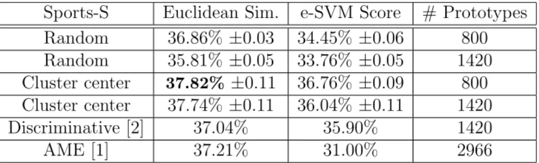
Discriminative Selection: Moreover, we use discriminative patch [2] algorithm to select the prototypes. As seen in Table 5.1 and Table 5.2, the results are better than random selection whereas using the cluster centers is better than using discriminative clips even if the number of prototypes are the same, and cluster centers being much better with careful selection of number of prototypes. AME Selection: Finally, we use AME [1] approach to select the prototypes by eliminating irrelevant and noisy data. We select purified positive instances as our exemplars. According to experimental results which are given in Table 5.1

UCF-S Euclidean Sim. e-SVM Score # Prototypes Random 53.81% _±1.21 51.63% _±1.19 430 Random 53.54% ±1.25 51.54% ±1.20 600 Cluster center 55.27% _±0.61 53.81% _±0.53 430 Cluster center 56.36% _{±0.90 53.00% ±0.87} 600 Discriminative [2] 54.18% 53.45% 430 AME [1] 54.18% 54.18% 867

Table 5.1: Results for UCF-S dataset. Baseline is: 48.72% Sports-S Euclidean Sim. e-SVM Score # Prototypes Random 36.86% ±0.03 34.45% ±0.06 800 Random 35.81% ±0.05 33.76% ±0.05 1420 Cluster center 37.82% _{±0.11 36.76% ±0.09} 800 Cluster center 37.74% _±0.11 36.04% _±0.11 1420 Discriminative [2] 37.04% 35.90% 1420 AME [1] 37.21% 31.00% 2966

Table 5.2: Results for Sports-S dataset. Baseline is: 33.62%

and Table 5.2, AME is also useful since it provides the most relative instances for the action class of interest. However, still we have the best improvements by choosing prototypes from k-means cluster centers.

Discussion on the proposed methods: An illustration of prototype selection methods for Sport-S dataset is given in Figure 5.2. We get insufficient prototypes from random selection since there are noisy or irrelevant data in “basketball” class such as an interview, a fan made video or a ceremony. Selecting cluster centers provides elimination by giving more importance to real action videos. Further-more, by choosing discriminative members with discriminative selection [2] and AME [1], we were able to select efficient prototypes compared to random selection. Note that, for almost all the experiments, using Euclidean similarity values was better than using Exemplar SVM(e-SVM) scores for representation. It is because for an accurate model learning with exemplar SVMs, the negative data should be e↵ective enough and it should include a large range of variety. Therefore,

UCF-S Sports-S

Baseline Prototype Baseline Prototype Archery 41.37% 24.13% 28.12% 32.50% Basketball 20.00% 40.00% 28.35% 34.32% Billiards 79.31% 93.10% 13.86% 24.75% Bowling 59.37% 71.87% 55.38% 48.46% Fencing 60.00% 75.00% 47.10% 60.86% Golf 24.24% 45.45% 2.38% 4.76% HorseRacing 68.00% 64.00% 26.42% 25.00% Kayaking 73.33% 76.66% 41.34% 42.30% Skiing 22.22% 26.62% 45.25% 50.36% Surfing 50.00% 50.00% 21.13% 22.76% Overall 48.72% 56.36% 33.62% 37.82%

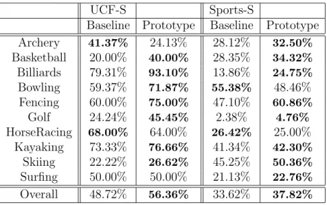
Table 5.3: Class based accuracies on UCF-S and Sports-S for prototype repre-sentation.

setting the global negative data in terms of the amount and the quality, is slightly difficult. Our intuition, Euclidean similarity is a much simple method to use and gives consistent results. However, it is important to be careful about the curse of dimensionality while using Euclidean distance.

Thus, in the follow-up experiments we used Euclidean similarity values as our representation method, and cluster centers as prototypes with 600 for UCF-S and 800 for Sports-S. As Table 5.3 shows, for almost all categories prototype based representation is better than using low-level features. Lower results for Sports-S dataset is due to the difficulty of the dataset compared to clean UCF-S dataset. However, other than for archery and bowling, we see a similar pattern for the individual actions.

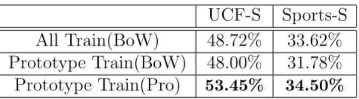
Choosing only the prototypes as training data: Besides using the pro-totypes for representation, we also experiment using the propro-totypes directly as training data to reduce the data size. As shown in Table 5.4, compared to us-ing all the examples in the trainus-ing data (1084 for UCF-S and 3296 for Sports-S respectively) with the low-level BoW representation, using only prototypes (600 for UCF-S and 800 for Sports-S respectively) with the same representation gives

UCF-S Sports-S All Train(BoW) 48.72% 33.62% Prototype Train(BoW) 48.00% 31.78% Prototype Train(Pro) 53.45% 34.50%

Table 5.4: Prototypes as training data.

lower performances. However, especially for UCF, it is not significant in spite of the reduced number of training examples. This shows us that, with the careful selection of the training data we can reduce the e↵ort required for labeling. More importantly, when we use the prototypes as representation as well, we can also increase the classification performance.

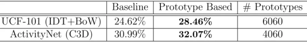
Experiments on benchmark datasets: In addition to our detailed experi-ments on subset datasets as UCF-S and Sports-S, we give the improved results on the benchmark datasets such as UCF-101 and ActivityNet. We show the comparison of baseline and prototype based representation method results in Ta-ble 5.5. Moreover, class based enhancements of UCF-101 dataset can be observed in Figure 5.3. Note that, we use the k-means cluster center selection method with k = 60 and Euclidean Similarity representation since they have proven to give the best results for UCF-101.

For Activitynet baseline, we utilize computed deep-level C3D features which are explained in 5.2.2. By this way, we show, even with the deep-level advance features, prototype based representation can help us to obtain better classification scores. We determine the best cluster number empirically as k = 20 for this dataset.

Note that, we have lower improvements on weakly-labeled datasets such as Sports-S and ActivityNet than the enhancement on UCF-101. This di↵erence is due to the noisy content of the datasets since validation and test data have also these irrelevant samples. Consequently, in the prediction phase, we have lower chance to decrease the e↵ect of noise despite the accurate models. However, since UCF-101 is a hand-crafted dataset, our contribution results in a more e↵ective

Baseline Prototype Based # Prototypes

UCF-101 (IDT+BoW) 24.62% 28.46% 6060

ActivityNet (C3D) 30.99% 32.07% 4060

Table 5.5: Prototype based representation results for UCF-101 and ActivityNet. manner.

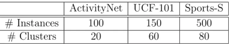
Discussion on cluster number selection: As shown in experimental re-sults(Fig. 5.1), the chosen cluster number is very e↵ective on an accurate rep-resentation. While selecting the cluster number, it is important to consider the number of instances in each class. In order to select a useful prototype, cluster centers should be representative. Therefore, the more clusters we have the more impure clusters we get according to the number of instances in the class and it provides insufficient cluster centers which influence prototype quality.

For example, ActivityNet has approximately 100 videos in per class and if we choose k = 80, our cluster centers will be irrelevant since we create clusters from noisy instances, too. However, according to the results, k = 20 is a good number by the means of eliminating the bad influence of spuriour samples. Likewise, Sports-S dataset has 500 examples in each class so that we should select higher number of cluster centers for an accurate representation. Hence, the e↵ective number of clusters di↵ers with respect to the dataset.

In addition to instance number, we should consider the content of the classes. For instance, UCF-101 can be regarded as a purer dataset than the others. So, high number of clusters will not e↵ect the results that much. In contrast, Ac-tivityNet and Sports-S are noisy and weakly-labeled datasets so that we should be careful while selecting the cluster number. A complete report of best cluster numbers for each dataset can be seen in Table 5.6.

ActivityNet UCF-101 Sports-S

# Instances 100 150 500

# Clusters 20 60 80

Table 5.6: The best cluster numbers and the number of instances in per class for each dataset.

5.2

Analysis of AME for Action Recognition

For this experiment, we get state-of-the-art results by applying the same reported settings to related datasets. After that, we observe the achievements of AME [1] on computed representations for action recognition. We basically apply AME on train set in order to eliminate irrelevant or noisy instances iteratively after the representation process for each class separately. We use a global negative set against given positive train set for a class. We create the negative dataset by taking all class instances except the positive class by applying one-vs-rest approach.

We compute baseline models by using raw train data in learning phase and then we use given test data for the prediction part. We purify the training data from noisy instances to learn better models by using AME [1] and we do the prediction phase again over the models which are learned from pure training set. Note that, we only change the training data for learning better models in AME. Therefore, we apply the same evaluation process after using the reported methods.

5.2.1

Parameter Tuning

We did detailed experiments on AlexNet UCF-101 and ActivityNet features by tuning AME [1] parameters which are explained in Section 2.2.2. The graph-ics that show e↵ects of the parameters on classification accuracy are given in Figure 5.4.

Here, we observe that higher min elimination ratio values decrease the recog-nition accuracy on UCF-101 dataset which includes less noisy data than Activi-tyNet. For the big min elimination ratio numbers, AME eliminates the relevant data, too. Therefore, this situation is inappropriate for datasets like UCF-101. However, to provide a more purified dataset and to get higher action recognition results, ActivityNet needs bigger number of elimination.

M1 selection ratio and M2 selection number should be selected carefully since they determine the number of eliminated instances for M1 _{and M}2 _{models. For}

the comparisons, we choose the parameters according to obtained results which give the maximum classification accuracy.

5.2.2

Comparisons and Results

We compare the baseline results with AME [1] results. Note that, since this method improves the learning on given features, we do not provide the best results for datasets. We only show the enhancement over the stated baseline results in the literature. In order to do that, firstly, we get the same baseline results with the same methods. Then, we apply AME on resulting features as explained before. In the following, we give results for each dataset separately. UCF-101: Since we did experiments by using both low-level and deep-level features for this dataset, we give three di↵erent baselines and AME [1] results in Table 5.7. Here, we take the given result in [33] as IDTF baseline. Furthermore, for AlexNet and C3D deep feature results, we take the reported results in [35].

In Table 5.7, we present results from which we got the highest improvement on the baseline when we select min elimination ratio=0.1 , M1 selection ratio=0.4 and M2 selection number=1 . The reported AME result on IDT representation is calculated by using the same parameters which are determined by fine tuning.

Moreover, we compare our AME result with discriminative patch approach introduced by Singh et al. [2] for discovering representative and discriminative

Method Baseline AME [1] IDT + FV + Linear SVM 84.80% [33] 85.14% AlexNet(fc-6) + Linear SVM 68.80% [35] 69.09% C3D(fc-6) + Linear SVM 82.30% [35] 83.47%

Table 5.7: UCF101 classification results after AME [1] elimination. In the first column the state-of-the art results are given and second column reports AME results over these baselines.

Method Baseline AME [1] Discriminative [2] AlexNet(fc-6) 68.80% [35] 69.09% 52.33%

Table 5.8: Comparison of AME [1] and Discriminative Patch method we imple-mented based on the algorithm that is given in [2].

patches from images for a mid-level representation. We adapt this method for videos and we consider each video as a patch in the given algorithm [2]. The comparisons on AlexNet features with our implementation of discriminative patch method is given in Table 5.8. Note that, we used our implementation which is based on given algorithm in [2] and we adapted this to video classification. The large drop on the performance with discriminative patch idea is likely to occur due to the insufficiency of the data required by that method.

ActivityNet: For this dataset, we compare our results with given state-of-the-art result in [52]. Here, we compute the same features which are extracted from AlexNet architecture by using pre-trained ImageNet model. We employ fc-6 layer features for our baseline result. The accuracy result for this method is reported as 28.3% by [52]. However, our baseline result is 25.68%. Our observation for this variety is using di↵erent sample clips from videos as explained in 4.1. Therefore, we give the improvements over this baseline result in Table 5.9.

Moreover, we calculate C3D (3D Conv) features by using the provided frame-work. As far as we know, there are not any reported results for ActivityNet C3D feature evaluation. Therefore, we give our calculated baseline result in Table 5.9. We feed approximately 7 clips in 16 frames long to the network for each video

Method Baseline Accuracy (%) AME [1] AlexNet(fc-6) + Linear SVM 25.68% 27.52%

C3D(fc-6) + Linear SVM 30.99% 33.19%

Table 5.9: Action recognition results on ActivityNet after AME [1] elimination. First column reports baseline classification results for deep level features and second column gives improvements of AME.

as done in [35]. After extracting 3D deep features for each clip, we average them for a video level description which is followed by L2 normalization. Then, we do multi-class Linear SVM classification.

We show the results in Table 5.9 by selecting the parameters which give the highest results for AME [1] after fine tuning as follows: min elimination ratio=0.4 , M1 selection ratio=0.7 and M2 selection number=10 . The reported AME result on C3D representation is calculated by using the same parameters. Furthermore, we give the class based comparisons in Figure 5.5.

Discussion: As it can be seen from the results, we have less improvement on UCF-101 compared to ActivityNet. The reason is that ActivityNet dataset is more challenging since it is directly collected from the internet. However, UCF-101 is a hand-crafted dataset and there are a few challenging instances that can decrease accurate model learning instead of the noisy and irrelevant data. Therefore, we can say that eliminating 10 instances from each class is enough for a better learning by looking Figure 5.4.

Here, if we start to increase M1 selection ratio, algorithm eliminates the rele-vant data as well. Hence, we got lower classification accuracy results. An example of this situation can be seen in Figure 5.6. Since we do not want to loose infor-mative instances, choosing M1 selection ratio small is a good idea for a less noisy dataset. Furthermore, AME can be used as an informative and representative instance selector since it iterates through the entire data in order to determine the best set which has the data furthest from negative set. Meanwhile, it removes the instances that can decrease the accurate model learning.

In contrast, for a noisy dataset, the more we eliminate the data the higher scores we get. As it can be seen from the Figure 5.4, for ActivityNet dataset, we got the highest prediction scores by eliminating 40 instances from each class since the M1 selection ratio=0.4 . Also, the value of M2 selection number varies according to dataset. For example, while eliminating only 1 data in per iteration is preferable for UCF-101, for ActivityNet dataset we have higher results when 10 instances are eliminated. The reason is that again for UCF dataset we do not want to eliminate relevant instances and if iterations finish so early, we would not be able to prune actual challenging data. So, iterative approach provides us better results.

Figure 5.7 shows sample video clips from ActivityNet dataset that are selected as category references or eliminated as irrelevant items. As seen from the ex-amples, AME [1] successfully keeps the videos that are representative for the category while eliminating the videos that are not descriptive for the category or could describe more than one category. Compared to the performance of the orig-inal training data, the new data purified by AME [1] is much better in these cases. As depicted in Figure 5.6, in some cases, especially on relatively clean UCF-101 dataset, AME may remove some of the relevant items besides the irrelevant ones resulting in lower performances for small number of classes.

200

400

600

800

1000

Number of Prototypes

53

53.5

54

54.5

55

55.5

56

56.5

Classification Accuracy

UCF-S

random

cluster centers

200

400

600

800

1000

1200

Number of Prototypes

34.5

35

35.5

36

36.5

37

37.5

38

Classification Accuracy

Sports-S

random

cluster centers

Figure 5.1: Classification results for di↵erent number of prototypes for both ran-dom and cluster center selection. As it can be seen from the graphics, the quality of the prototypes are more important than the amount of them.

K-means Cluster Center Selection Random Selection

Discriminative Selection (High Scored Cluster Members)

AME Selection

Figure 5.2: Resulting exemplars of di↵erent selection methods for “basketball” action class in Sports-S dataset.

0 25 50 75 100 Ap p lyEye Ma ke u p Ap p lyL ip st ick Arch e ry Ba b yC ra w lin g Ba la n ce Be a m Ba n d Ma rch in g Ba se b a llPi tch Ba ske tb a ll Ba ske tb a llD u n k Be n ch Pre ss Bi ki n g Bi lli a rd s Bl o w D ryH a ir Bl o w in g C a n d le s Bo d yW e ig h tSq u a ts Bo w lin g Bo xi n g Pu n ch in g Ba g Bo xi n g Sp e e d Ba g Bre a st St ro ke Bru sh in g T e e th C le a n An d Je rk C lif fD ivi n g C ri cke tBo w lin g C ri cke tSh o t C u tt in g In Ki tch e n D ivi n g D ru mmi n g F e n ci n g F ie ld H o cke yPe n a lt y F lo o rG ymn a st ics F ri sb e e C a tch F ro n tC ra w l G o lf Sw in g H a ircu t H a mme rT h ro w H a mme ri n g H a n d st a n d Pu sh u p s H a n d st a n d W a lki n g H e a d Ma ssa g e H ig h Ju mp H o rse R a ce H o rse R id in g HulaHoop _IceD a n ci n g Ja ve lin T h ro w Ju g g lin g Ba lls Ju mp R o p e Ju mp in g Ja ck Ka ya ki n g Kn it ti n g BoW Prototype 0 25 50 75 100 L o n g Ju mp Lunges Mi lit a ryPa ra d e Mi xi n g Mo p p in g F lo o r N u n ch u cks Pa ra lle lBa rs Pi zza T o ssi n g Pl a yi n g C e llo Pl a yi n g D a f Pl a yi n g D h o l Pl a yi n g F lu te Pl a yi n g G u it a r Pl a yi n g Pi a n o Pl a yi n g Si ta r Pl a yi n g T a b la Pl a yi n g V io lin Po le V a u lt Po mme lH o rse Pu llU p s Pu n ch Pu sh U p s Rafting R o ckC limb in g In d o o r R o p e C limb in g Rowing Sa lsa Sp in Sh a vi n g Be a rd Sh o tp u t Ska te Bo a rd in g Ski in g Ski je t SkyD ivi n g So cce rJu g g lin g So cce rPe n a lt y St ill R in g s Su mo W re st lin g Su rfin g Sw in g T a b le T e n n isSh o t T aiChi T e n n isSw in g T h ro w D iscu s T ra mp o lin e Ju mp in g T yp in g U n e ve n Ba rs V o lle yb a llSp iki n g W a lki n g W it h D o g W a llPu sh u p s W ri ti n g O n Bo a rd Yo Yo

Figure 5.3: Class based accuracy results for UCF-101 dataset with prototype representation. The results are given for cluster center selection when k = 60 and Euclidean similarity representation.