Selçuk J. Appl. Math. Selçuk Journal of Vol. 10. No.1. pp. 75-84, 2009 Applied Mathematics
Edgeworth Series Approximation for GammaTtype Chance Constraints Mehmet Yılmaz
Ankara University, Faculty of Science, Statistics Department, Ankara, Turkey e-mail: yilm azm @ science.ankara.edu.tr
Received: April 28, 2008
Abstract. We introduce two expansions for approximation to distribution of sum of weighted Gamma variates based on Central Limit Theorem. For more than two weighted components, the exact distribution is more complicate for some application areas like chance constrained programming. This lead us to give two expansions to transform Gamma type chance constrained stochastic model into its deterministic equivalent.
Key words: Gamma distribution, edgeworth expansion, central limit theorem, chance constrained programming, stochastic programming
2000 Mathematics Subject Classification. 60E05, 90C15, 62E17, 60E07. 1.Introduction
The distribution of non negative weighted sum of independent Gamma variates arises in many application areas such as reliability of systems, industrial pro-duction process, engineering, etc. Literature review of this subject can be found in Johnson et al. (1994).
Common problem in the practical application of statistics is the difficulty of find-ing exact distribution of weighted sum. Even if one can find exact distribution of weighted sum, its complexity can not lead to solve some problems in CCP when the number of components is more than two for gamma variates. Therefore, normal approximation commonly used in application of statistics. This lead us to introduce edgeworth series expansions based on normal approximation for such a distribution. We will also use central limit theorem and compare these three approximation methods with exact distribution of weighted sum up to four components in second section. We will recall CCP in third section, since aimed to finding deterministic equivalent of Gamma type CCP model and illustrative examples are also given.
2. Approximations of Weighted Sum of Gamma Variates
In this section, we will introduce and extend three expansion methods based on normal approximation for the independent but not identical random variables. First method is related to generalized central limit theorem, second is called first term edgeworth expansion, and the third method is called second term edgeworth expansion.
Theorem1. (Generalized Central Limit Theorem). Let 1 2 be
con-tinuous and independent random variables such that ||2 ∞ ( = 1 2 )
(1) à P =1 ≤ ! = ó ()2 ´− 1 2 " P =1 − à P =1 !# ≤ ! = Φ ()
where Φ stands for standard normal distribution, ()2 denotes
P
=1
(− ())2
here stands for
− P =1 ()2
(Lehmann, 1999 and Feller, 1966).
Theorem2. Let 1 2 be independent continuous random variables
such that ||4 ∞ ( = 1 2 ). denotes distribution function of
standardized sum = P =1 (− ()) v u u t à P =1 !
for large values of , then the first term edgeworth series expansion is (2) () = Φ() −6√3Φ(3)()
the second term edgeworth series expansion is (3) () = Φ() −6√3Φ(3)() + 1 ³ 4 24Φ (4)() +2 3 72Φ (6)()´ where = 2−1 = 1 ln () (Wallace, 1958).
2.1 Set-up for Weighted Gamma Variates
Consider distributed as ( ), then the density function is
() = 1 Γ() −1 − 0 and 0
Suppose that ’s are non negative real numbers then for = 1 2 , ∼
( ) Hence characteristic function of P =1 denoted by is as follows () = Q =1 Ã 1 − 12 2 !− −1 1 2 2
here 1and 2denote P =1 and P =1 () 2
respectively. Third and
fourth cumulants are K3= 2
P =1 () 3 3 2 2 , and K4= 6 P =1 () 4 2 2 In the view of Theorem1, µ P =1 ≤ ¶ is approximated as (4) ( ≤ ) ≈ Φ() where =√−1
2. Now, we can reformulated (2) and (3)
(5) (≤ ) ≈ Φ() + ∙ 3(1−2) 6(2) 3 2 ¸ () (6) (≤ ) ≈ Φ() + ∙ 3(1−2) 6(2) 3 2 − 4(3−3) 242 2 − 32( 5 −103+15) 723 2 ¸ () here (·) denotes unit normal density function, and 3 and 4 stand for K3
and K4 respectively.
Suppose that a system contains two weighted components such as 1∼
(1 4) and 2∼ (2 3) distributed independently. We will first compare
these approximations with the exact distribution. The quantity of (21+
152≤ ) can be tabulated some values of . We can see that from table1, (5)
and (6) are not far from away exact distribution, but (4) is not. Here ED, NA, FE and SE denote exact distribution, normal approximation, first edgeworth and second edgeworth series expansions respectively.
TABLE 1. Computed probability for two weighted components
Secondly, consider a system with three components such as 1∼ (2 4)
2 ∼ (5 3), 3 ∼ (1 2) distributed independently then the
quantity of (051+ 082+ 3≤ ) can be computed and tabulated below
(Table2).
TABLE 2. Computed probability for three weighted components
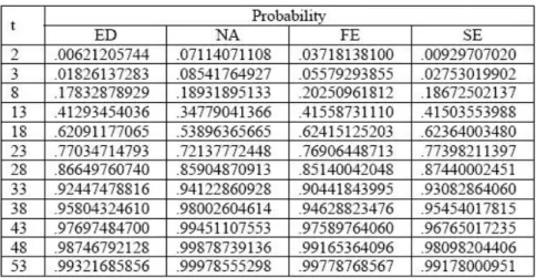
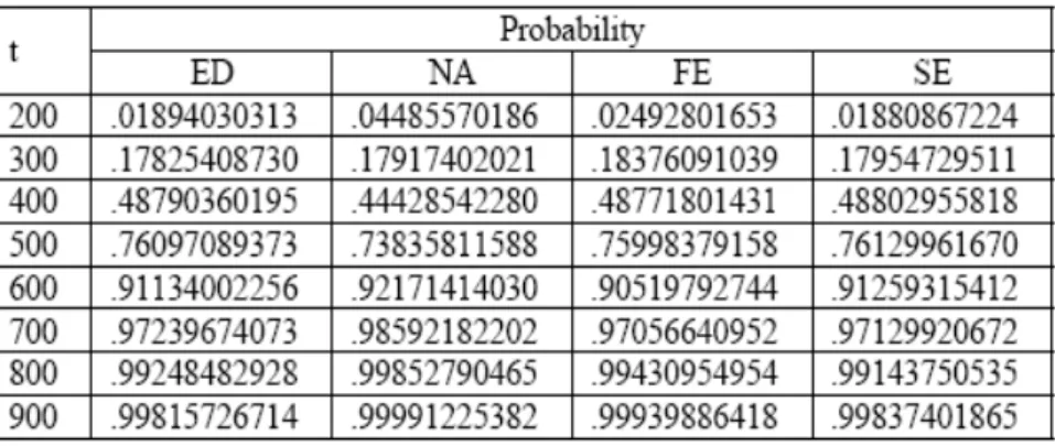
Thirdly, a system contains four weighted components such as 1∼ (2
1) 2∼ (3 3), 3∼ (1 1) and 4∼ (7 4) distributed
independently. The computed probability of 121+ 072+ 093+ 1154
TABLE 3. Computed probability for four weighted components
For more than three components, exact distribution is quite complex in appli-cation areas like CCP. It can be emphasized that even if these approximations yield better result for large sample theory, we can see that for = 2 3 4 edge-worth series results are closely to reach exact distribution’s results. Thereby FE and SE methods can be applied to solving CCP problem by transforming chance constraints in model into its deterministic equivalents.
3. Deterministic Model for Gamma Type Chance Constraints
We first introduce chance constrained stochastic programming. Stochastic pro-gramming deals with the case that input data (prices, right hand side vector, technologic coefficients) are random variables. As parameters are random vari-ables a probability distribution should be determined. There are two approaches used frequently for changing stochastic programming problem into determinis-tic programming problem. These are chance constraint programming and two staged programming (Hillier and Lieberman, 1990).
CCP which is one of stochastic programming methods contains fixing the certain appropriate levels for random constraints. For this reason, it is generally used for modeling of technical or economic systems. The practices contain economic planning, input control, structural design, stocking management, air and water quality management problems. In chance constraints, each constraint can be realized with a certain probability. The original mathematical programming model, max(min)() = X =1 P =1 ≤ for = 1 2 ≥ 0 = 1 2
was well defined. Constraints replaced by
(7) Ã P =1 ≤ ! ≥ 1 − for = 1 2
where the are specified probabilities. Here, it is assumed that decision
variables are deterministic, technologic coefficients, or right hand side,
or are random variables or both of and are random variables (see,
Charnes and Cooper, 1959).
We consider the CCP problem when the ’s are random variables distributed
( ) = 1 2 , and , are constant. Deterministic
equiva-lents of (7) will be obtained in this case. The equivalent deterministic problem is obtained by five methods and these are compared by values of the objective function. We can establish for only two and three components since the exact distribution can not appropriate in solving CCP for more than three compo-nents.
Consider k th chance constraint given in model (7)
(8) Ã P =1 ≤ ! ≥ 1 −
one can find deterministic equivalent of (8), the problem may turn to find dis-tribution of
P
=1
. Therefore, suggested first method is finding exact
distri-bution.
Method I: (Exact Distribution, (ED)). This method will be obtained for two and three components. 2denotes distribution of 11+ 22
(9) 2() = R 0 21+2−1− 11 µ 2 1+ 2 µ 1 11− 1 22 ¶¶ where 2= Γ(1+2)(1 1
1)1−1(22)2−1 and 3 denotes distribution of 11+
22+ 33 (10) 3() = R 0 31+2+3−1− 11( ) where ( ) is defined by R 0 3−1 (1 − )1+2−1− 33− 11 (2 1+ 2 (1 − )12) and 12= ³ 1 11 − 1 22 ´ can be defined.
Method II: (Central Limit Theorem, (NA)). Deterministic equivalent of (8) can be obtained by using normalization, from (4) as follows
(11) Φ³√−1 2 ´ ≥ 1 − ⇒ Φ−1(1 − )√ 2+ 1≤ 1− P =1 = 0 2− P =1 () 2 = 0
Method III: (First Term Edgeworth Series Expansion, (FE)). From (5), we can rewrite (8) (12) 1− P =1 = 0 2− P =1 () 2 = 0 −√−1 2 = 0 3= 2 P =1 () 3 = 0 Φ() + ∙ 3(1−2) 6(2) 3 2 ¸ −52 √ 2 ≥ 1 −
Method IV: (Second Term Edgeworth Series Expansion, (SE)). Deterministic equivalent of (8) can be rewritten from (6) as follows
(13) 1− P =1 = 0 2− P =1 () 2 = 0 −√−1 2 = 0 3= 2 P =1 () 3 = 0 4= 6 P =1 () 4 = 0 Φ() + ∙ 3(1−2) 6(2) 3 2 − 4(3−3) 242 2 − 32( 5 −103+15) 723 2 ¸ −52 √ 2 ≥ 1 −
Method V: (Sengupta’s Method, (SM)). Sengupta (1970) has offered for trans-forming chi-square type chance constraint into its deterministic equivalent. Let 1 2 be independent and distributed 2()then (
P =1 ≤ ) ≥ 1 − can be transformed to (14) µ P =1 () ¶ − 2() µ P =1 2 () ¶ ≥ 0
here () = , = P =1 and 2
() denotes inverse distribution function with
degrees of freedom on the 1 − level.
Gamma variates can easily represented by chi squared variates, such that, if ∼ ( ) then 2 ∼
2
(2). Hence, equivalent deterministic
constraint of (8) can be given in the view of (14) respectively,
(15) (1) − 1 2 2 (2 P =1 ) 2≥ 0
inequality is reversed for the min problem.
In the next section, we will give illustrative examples for five methods and compare with each other.
4. Numerical Examples
Example1. Consider the CCP problem as follows:
(16)
max (1 2) = 1+ 2
(11+ 22≤ 2) ≥ 08
1 2≥ 0 1 2≤ 1
where 1 and 2 distributed as (1 4) and (2 3) respectively.
Solutions have been obtained by using Lingo 9.0 and Matlab presented as in Table 4.
TABLE 4. Solutions for Model (16)
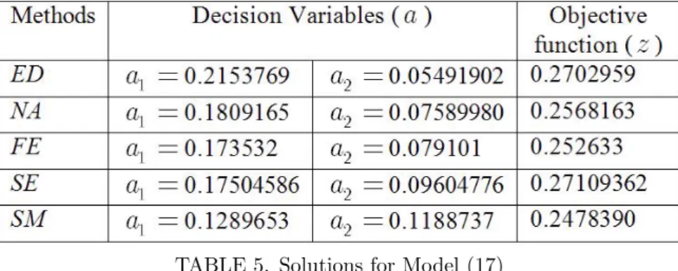
Example2. Consider the CCP problem with two chance constraints as follows:
(17) max (1 2) = 1+ 2 (111+ 212≤ 2) ≥ 085 (121+ 222≤ 1) ≥ 096 1 2≥ 0 1 2≤ 1 where 11∼ (1 4), 12 ∼ (2 3), 21∼ (1 1), 22 ∼ (1 2)
TABLE 5. Solutions for Model (17)
Example3. Consider the CCP problem for three components as follows:
(18)
max (1 2 3) = 1+ 2+ 3
(11+ 22+ 33≤ 1) ≥ 08
1 2 3≥ 0 1 2 3≤ 1
where 1∼ (1 4), 2∼ (2 3) and 3∼ (1 2)
TABLE 6. Solutions for Model (18) 5. Conclusion
In this present work, we have introduced two expansions based on normal ap-proximation for the weighted sum of Gamma variates. These are considered as an application of CCP problem when only ’s are assumed to be independently
distributed Gamma random variables. Since the exact distribution of weighted sum of Gamma variates can be convenient for two and three components, NA, FE, SE and SM methods can be compared with ED. It can be concluded from the illustrative examples that FE and SE give better approximation to the ED’s results for small values of , however ED and SE are related to large sample theory. These give eligible results for the Gamma type CCP problem.
As can be seen in Table 4,5, and 6 above, which summarizes the solution of the (16), (17) and (18) models for five methods. The solutions of deterministic model obtained by using NA, SM are extremely far away from the ED, but FE and SE solutions are close to ED solutions. Furthermore, ED method is
quite complex for large values of , ED method is also difficult to perform any other distribution such as Chi Square. FE and SE are both useful for large . Therefore SE method can be recommended to converting chance constraint into its deterministic constraint for Gamma type chance constrained stochastic programming.
References
1. Charnes A. and Cooper W. W. (1959): Chance-constrained programming, Man-agement Sci. 5, 73-79.
2. Feller, W. (1966): An Introduction to Probability Theory and Its Applications, Volume II. (John Wiley and Sons, Inc. New York, London).
3. Johnson, N.L. Kotz, S. and Balakrishnan, N. (1994): Continuous Univariate Dis-tributions I., Second Ed. New York: John Wiley and Sons.
4. Hillier, F.S. and Lieberman, G.J. (1995): Introduction to Mathematical Program-ming. Hill Publishing Company, New York.
5. Lehmann, E.L. (1999): Elements of Large Sample Theory, Springer Verlag, New York Inc.
6. Sengupta, J.K. A. (1970): Generalization of some distribution aspects of chance constrained linear programming, International Economic Review, 11, 287-304. 7. Wallace, D. L. (1958): Asymptotic approximations to distributions, The Annals of Mathematical Statistics, 29, No. 3, p. 635-654.