Dynamics of a plant-herbivore model with differential-difference equations

(1)

APPLIED & INTERDISCIPLINARY MATHEMATICS | RESEARCH ARTICLE

Dynamics of a plant–herbivore model with

differential–difference equations

S. Kartal1_*

Abstract: This paper studies the behavior of a plant–herbivore model including both

differential and difference equations. To analyze global behavior of the model, we

consider the solution of the system in a certain subinterval which gives to system of

difference equations. The boundedness characters, the periodic nature, both

local and global stability conditions of the plant–herbivore system are investigated.

Numerical studies indicate that the system exhibits Neimark–Sacker bifurcation for

different parameter values in certain regions.

Subjects: Applied Mathematics; Dynamical Systems; Mathematical Modeling; Mathematics & Statistics; Science

Keywords: plant–herbivore system; difference equation; stability; Neimark–Sacker bifurcation

Mathematics subject classifications: 37N25; 39A28; 39A30 1. Introduction

Classical approaches to modeling plant–herbivore interactions are based on predator–prey system (Caughley & Lawton, 1981; May, 2001). This interaction has been described in much research using discrete and continuous model (Agiza, ELabbasy, EL-Metwally, & Elsadany, 2009; Chattopadhayay, Sarkar, Frıtzsche-Hoballah, Turlıngs, & Bersıer, 2001; Danca, Codreanu, & Bakó, 1997; Das & Sarkar, 2001; Edelstein-Keshet, 1986; Feng, Qiu, Liu, & DeAngelis, 2011; Lebon, Mailleret, Dumont, & Grognard, 2014; Li, 2011; Liu, Feng, Zhu, & DeAngelis, 2008; Mukherjee, Das, & Kesh, 2011; Ortega-Cejas, Fort, & Méndez, 2004; Owen-Smith, 2002; Saha & Bandyopadhyay, 2005; Sui, Fan, Loladze, & Kuang, 2007; Sun, Chakraborty, Liu, Jin, & Anderson, 2014; Zhao, Feng, Zheng, & Cen, 2015). The model of Li (2011) is a system of differential equations with Holling type II functional response where the plant toxin’s influence in herbivores is considered. In study, Mukherjee et al. (2011) have used discrete time model with Holling type II functional response for describing the plant–herbivore interaction.

*Corresponding author: S. Kartal, Faculty of Education, Department of Mathematics, Nevsehir Haci Bektas Veli University, Nevsehir 50300, Turkey E-mail: senol.kartal@nevsehir.edu.tr

Reviewing editor:

Amar Debbouche, Guelma University, Algeria

Additional information is available at the end of the article

ABOUT THE AUTHOR

Senol Kartal is an associate professor in Nevsehir Haci Bektas Veli University, Turkey. His PhD thesis is about the population dynamics (Modeling of Tumor Immune System Dynamics Using System of Difference Equations and Its Stability Analysis). His research interests are related to population dynamics, discrete and continuous dynamical system, and bifurcation theory. He has published his research contributions in some internationally renowned journals whose publishers are Elsevier, Taylor & Francis, Wiley, and other journals.

PUBLIC INTEREST STATEMENT

In this study, we consider a plant–herbivore model which consists of ordinary differential equations. Our aim is to build a better understanding of how both discrete and continuous times affect the dynamic behavior of plant–herbivore interactions. Therefore, we add discrete time to this model and obtain a system of differential equations with piecewise constant arguments which gives system of difference equations. The boundedness characters, the periodic nature, both local and global stability conditions of the system are investigated.

Received: 22 October 2015 Accepted: 21 December 2015 First Published: 19 January 2016

(2)

It is well known that discrete time models governed by difference equations are more appropriate than the continuous time models when the populations have non-overlapping generations. So, a signifi-cant number of the study on the mathematical models of plant–herbivore interactions are described by the system of difference equations (Agiza et al., 2009; Danca et al., 1997; Mukherjee et al., 2011; Sui et al., 2007). In addition, working with difference equations instead of differential equations allows us to some advantages. Discrete dynamical models can bring about easier computational methods for the persistence, periodic solutions, boundedness, local and global properties of the dynamical system.

In plant–herbivore interactions, delay differential equations may widely occur due to herbivore dam-age and deployment of inducible defenses (Das & Sarkar, 2001; Ortega-Cejas et al., 2004; Sun et al., 2014). From this point of view, Sun et al. (2014) and et all have constructed a reaction-diffusion model with delay governed by system of partial differential equations where the effect of time delay on the herbivore cycles is investigated. In addition, the properties of delay differential equations are very close to differential equation with piecewise constant arguments. In Cooke and Györi study (1994), it was pointed out that these equations can be used to get approximate solutions to delay differential equations that include discrete delays. In such biological situations, dynamics of growth and death of populations can be described by differential equations otherwise, difference equations may reflect the interaction of two populations such as competition or predation phenomena (Gurcan, Kartal, Ozturk, & Bozkurt, 2014; Kartal & Gurcan, 2015). In the literature, various types of biological model consisting of differential equations with piecewise constant arguments have been analyzed using the method of reduction to discrete equations (Busenberg & Cooke, 1982; Gopalsamy & Liu, 1998; Gurcan et al., 2014; Kartal & Gurcan, 2015; Liu & Gopalsamy, 1999; Öztürk, Bozkurt, & Gurcan, 2012).

In the present paper, our aim is to build a better understanding of how both discrete and continu-ous times affect the dynamic behavior of plant–herbivore interactions. So we will reconsider the model (see Chattopadhayay et al., 2001)

as a system of differential equations with piecewise constant arguments such as

which include both differential and difference equations. In this model, x(t) and y(t) represent the density of plant and herbivore population, respectively,

[[

t]]

denotes the integer part of

t ∈ [0, ∞)

and all these parameters are positive. The parameter r, K, and

𝛼

is the intrinsic growth rate,

environ-mental carrying capacity, and specific predation rate of plant species, respectively. s represents the death rate of herbivores and

𝛽

is the conversion factor of herbivores (Chattopadhayay et al., 2001).

The logistic term

rx(t)

(

1 −

x(t) K

)

and the term sy(t) include only a continuous time for the growth of plant and for the death of herbivore, respectively. The predational form

𝛼x(t)y([[t]])

represent the loss of plant population and

𝛽x([[t]])y(t)

is conversion factor of herbivores which include both dis-crete and continuous time for a each populations. So the plant–herbivore interaction is considered in a certain subinterval and is modeled using a system of differential equations with piecewise con-stant arguments.

2. Local and global stability analysis

System (1.2) can be written an interval

t ∈ [n, n + 1)

as follows:

(1.1)

{

_dx dt

=

rx(t)

(

1 −

x(t) K

)

− 𝛼

x(t)y(t),

dy dt

= −

sy(t) + 𝛽x(t)y(t),

(1.2)

{

_dx dt

=

rx(t)

(

1 −

x(t) K

)

− 𝛼

x(t)y([[t]]),

dy dt

= −

sy(t) + 𝛽x([[t]])y(t),

(2.1)

{

_dx dt

−

x(t)(r − 𝛼y(n)) = −rkx

2

(

t),

dy y(t)

= ((𝛽

x(n) − s))dt,

(3)

where 1 K

=

k.

By solving each equations of the system (2.1) and letting

t → n + 1

, we obtain a system of differ-ence equations

System (2.2) reflects the dynamical behavior of the system of differential equations with piecewise constant arguments. So we will consider the system of difference equation to analyze the global behavior of system (1.2).

The equilibrium points of system (2.2) can be obtained as

We note that the positive equilibrium of the system exists if

𝛽 >

ks

. Now, we will find Jacobian matrix of the system to investigate the dynamic behavior of the model.

Theorem 2.1. The equilibrium points E0 and E1 are saddle point.

Proof At the equilibrium point E0, the Jacobian matrix is the form

The matrix J0 has eigenvalues 𝜆1=e

r_{, 𝜆}

2=e

−s_{. Hence}_𝜆

1>1 and 𝜆2<1 and consequently E0 is saddle

point. On the other hand, the Jacobian matrix J1 at the point E1 is

which gives eigenvalues 𝜆₁=e−r_{and 𝜆}

2=e −s+𝛽

k. Considering the condition _{𝛽 >}ks, we can say that E

1

is saddle point.

On the other hand, the Jacobian matrix J∗ at the positive equilibrium point E∗ is

which yields the following characteristic equation

Now, we can apply Schur–Cohn criterion to determine stability conditions of the system with char-acteristic equation p(𝜆).

Theorem 2.2 The positive equilibrium point E∗ of system (2.2) is local asymptotically stable if and only if

Proof From the Schur–Cohn criterion, E∗ is local asymptotically stable if and only if

(a) (2.2)

{

x(n + 1) =

x(n)(r−𝛼y(n)) (r−𝛼y(n)−rkx(n))e−(r−𝛼y(n)) +rkx(n)

,

y(n + 1) = y(n)e

𝛽x(n)−s

,

E

₀

= (0, 0),

E

₁

=

( 1

k

, 0

)

,

E

_∗

=

( s

𝛽

,

r

𝛼

(

1 −

ks

𝛽

))

.

J0= ( er ₀ 0 e−s ) . J 1= ( e−r −𝛼−e −r 𝛼 kr 0 e−s+𝛽 k ) J_∗= ( e−kr ̄x (−1+e−kr ̄x_)𝛼 kr 𝛽 ̄y 1 ) p(𝜆) = 𝜆2+ 𝜆 ( −1 − e−kr ̄x) +e−kr ̄x +(1 − e −kr ̄x )𝛼𝛽 ̄y kr =0. ks < 𝛽 < k + ks.

p(1) = 1 + e

−kr ̄x

+

(1 −

e

−kr ̄x

)𝛼𝛽 ̄

y

kr

− 1 −

e

−kr ̄x

< 0,

(4)

(b) (c) (d)

The condition (a), (b), and (c) gives the inequalities

and

which always hold under the condition 𝛽 >ks. From (d), we get

which reveal

This completes the proof. □

For the parameter values

r = 0.2, 𝛼 = 0.6, K = 5, 𝛽 = 0.01, s = 0.02

and using initial conditions

x(1) = 0.2, y(1) = 0.22

, it can be seen that the positive equilibrium point

( ̄

x, ̄y) = (2, 0.2)

is local asymptotically stable, where blue and red graphs represent population density of plant and herbi-vore population, respectively.

Theorem 2.3 Let {x(n), y(n)}∞

n=−1 be a positive solution of system (2.2); then

In addition, if y(n) < x(n), then y(n) ≤ er

k(er−1)e

𝛽er k(er−1)−s_.

Proof It can be easily seen that

Also, it can be shown that y(n + 1) ≤ er

k(er−1)e

𝛽er

k(er−1)−s under the condition y(n) < x(n).

p(−1) = 1 + e

−kr ̄x

+

(1 −

e

−kr ̄x

)𝛼𝛽 ̄

y

kr

+ 1 +

e

−kr ̄x

< 0,

D

+ 1

= 1 +

e

−kr ̄x

+

(

1 −

e

−kr ̄x

)

𝛼𝛽 ̄

y

kr

< 0,

D

− 1

= 1 −

e

−kr ̄x

−

(

1 −

e

−kr ̄x

)

𝛼𝛽 ̄

y

kr

< 0.

(2.3) p(1) = ( 1 −e−kr ̄x)_{𝛼𝛽 ̄}_y kr < 0, (2.4) p(−1) = 2 + 2e−kr ̄x + ( 1 −e−kr ̄x)_{𝛼𝛽 ̄}_y kr < 0 (2.5) D+ 1= 1 +e −kr ̄x + ( 1 −e−kr ̄x)_{𝛼𝛽 ̄}_y kr < 0 e−kr ̄x + ( 1 −e−kr ̄x)_{𝛼𝛽 ̄}_y kr < 1 𝛽 <k + ks. x(n) ≤ e r k(er −1) . x(n + 1) = x(n)[r − 𝛼y(n)]e r−𝛼y(n)

r − 𝛼y(n) + rkx(n)(er−𝛼y(n)−1)≤

[r − 𝛼y(n)]er−𝛼y(n)

rk(er−𝛼y(n)

−1) ≤

er k(er₋₁) .

(5)

Theorem 2.4 The system has no prime period-two solutions.

Proof On the contrary, suppose that the system (2.2) has a distinctive prime period-two solutions

where w1≠w2, and q1≠q2, and wi, qi are positive real numbers for i ∈ {1, 2}. Then, from system (2.2)

one has

Since q1≠q2, we have 𝛽w2−s ≠ 0 and 𝛽w1−s ≠ 0. From the second and last equation in the system,

we have

If q2 is written the above equation, we hold

This equation must satisfy

which is a contradiction 𝛽w2−s ≠ 0 and 𝛽w1−s ≠ 0.

Theorem 2.5 Let A1=r − 𝛼y(n) and A2= 𝛽x(n) − s. Suppose that the conditions of Theorem 2.1 hold

and (i) (ii) (iii) (iv) (v)

Then the positive equilibrium point of system (2.2) is global asymptotically stable. Proof We define a Lyapunov function as

where q = ( ̄x, ̄y) is positive equilibrium point of system (2.2).̄ The change along the solutions of the system is

…,(w1, q1), (w2, q2), (w1, q1), (w2, q2) … . ⎧ ⎪ ⎪ ⎪ ⎨ ⎪ ⎪ ⎪ ⎩ w1= w2[r−𝛼q2] [r−𝛼q2−rkw2]e −[r−𝛼q2]+rkw2 , q1=q2e 𝛽w2−s w2= w1[r−𝛼q1] [r−𝛼q1−rkw1]e −_[r−𝛼q1]₊_rkw 1 , q2=q1e 𝛽w1−s_, q21=q 2 2e 𝛽w₂−s−𝛽w₁+s_. q21=q 2 1e 𝛽w₁−s+𝛽w₂−s_. 𝛽w₁−s + 𝛽w₂−s = 0 Let y(n) < r 𝛼 and ̄x < A₁(1 + e−A1₎ 2rke−A1 for x(n) ∈ ( 0, 2 ̄xe −A1 1 + e−A1 ) , Let y(n) > r 𝛼and ̄x > −A₁(1 + e−A₁₎ 2rk(e−A1₋₁) for x(n) ∈ ( 2 ̄xe−A1 1 + e−A1 , 2 ̄x ) , Let y(n) > r 𝛼for x(n) ∈(2̄x, ∞),

Let A

₂

>

0 for y(n) ∈

(

0,

2 ̄y

1 + e

A2

)

,

Let A

₂

<

0 for y(n) ∈

(

2 ̄y

1 + e

A 2

, ∞

)

.

V(n) = [q(n) − ̄q]2_, _{n = 0, 1, 2 …}

(6)

From the first equation in (2.2), we hold;

By considering (i), (ii), and (iii), we have ΔV1(n) < 0. These imply that _n→∞limx(n) = ̄x. Additionally, we can

show that ΔV2(n) < 0 which gives _n→∞limy(n) = ̄y. 3. Bifurcation analysis

In this section, we investigate existence of stationary bifurcation (fold, transcritical, and pitchfork bi-furcation), period doubling bifurcation, and Neimark–Sacker bifurcation for the system (2.2). All of these bifurcations can be analyzed under the set of algebraic conditions that is called Schur–Cohn criterion. It is well known that the system may undergo stationary bifurcation if and only if

p(1) = 0

,

p(−1) > 0

,

D

+

1

> 0

and

D

−

1

> 0

. On the other hand, inequalities

p(1) > 0,

p(−1) = 0

,

D

+

1

> 0

and

D

−

1

> 0

give the conditions of period doubling bifurcation. But considering (2.3) and (2.4), it is easily seen that these conditions do not hold for the system. Therefore, stationary bifurcation and period doubling bifurcation do not exist for the system.

Now, we can investigate the existence of Neimark–Sacker bifurcation for the plant–herbivore model (Hone, Irle, & Thurura, 2010). The algebraic condition of Neimark–Sacker bifurcation can be obtained from the analysis of inequalities

p(1) > 0

,

p(−1) > 0

,

D

+

1

> 0

and

D

−

1

= 0

. In local stability analysis, we have already shown that the inequalities

p(1) > 0

,

p(−1) > 0

,

D

+

1

> 0

are always exist. There-fore, we will only analyse the equation

D

−

1

= 0

to determine Neimark–Sacker bifurcation condition. Theorem 3.1 System (2.2) undergoes Neimark–Sacker bifurcation if and only if

Proof This result comes from the analysis of D− 1=0.

Using the condition of Theorem 3.1 with the parameters given in Figure 1, we have the Neimark– Sacker bifurcation point as _{K = 102 (Figure}̄ ₂_).

ΔV(n) = V(n + 1) − V(n) = {q(n + 1) − q(n)}{q(n + 1) + q(n) − 2 ̄q}.

ΔV1(n) =[x(n + 1) − x(n)][x(n + 1) + x(n) − 2 ̄x]

= x(n)[(A₁− rkx(n))(1 − e−A1)][A

1(x(n) + x(n)e

−A1_{− 2 ̄xe}−A1)

+ rkx(n)(x(n) − 2 ̄x)(1 − e−A1_)].

̄k = 𝛽

1 + s.

Figure 1. Stable equilibrium point of the system for r = 0.2, 𝜶 = 0.6, K = 5, 𝜷 = 0.01, s = 0.02, x(1) = 0.2 and y(1) = 0.22. 0 100 200 300 400 500 600 0 0.5 1 1.5 2 2.5 3 x(n) y(n)

(7)

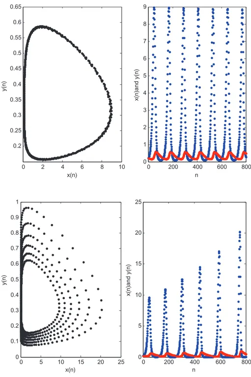
Figure 2. Stable limit cycle for r = 0.2, 𝜶 = 0.6, 𝜷 = 0.01, s = 0.02 and _{K = 102}̄ _. 0 2 4 6 8 10 0.2 0.25 0.3 0.35 0.4 0.45 0.5 0.55 0.6 0.65 x(n) y(n) 0 200 400 600 800 0 1 2 3 4 5 6 7 8 9 n x(n)and y(n)

Figure 3. Graph of the iteration solution of system (2.2) for r = 0.2, 𝜶 = 0.6, 𝜷 = 0.01, s = 0.02 and K = 200. 0 5 10 15 20 25 0 0.1 0.2 0.3 0.4 0.5 0.6 0.7 0.8 0.9 1 x(n) y(n) 0 200 400 600 800 0 5 10 15 20 25 n x(n)and y(n)

4. Result and discussion

In this paper, dynamics of a discrete-continuous time plant–herbivore model has been investigated. Local and global stability properties of the positive equilibrium point are analyzed. It is interesting to note that when conversion factor of herbivores becomes low then the system converges to a stable situation. On the other hand, we investigate possible bifurcation types for the system and observe that the system exhibits Neimark–Sacker bifurcation. This type of bifurcation has been observed in many plant–herbivore models (Liu et al., 2008; Saha & Bandyopadhyay, 2005; Zhao et al., 2015) and shows that periodic or quasi-periodic solutions occur as a result of a limit cycle.

(8)

In our manuscript, the parameter K (environmental carrying capacity of plant species) is determined as a bifurcation parameter. When the environmental carrying capacity of plant species reaches to

̄

K = 102

, the system enters a Neimark–Sacker bifurcation as a result of stable limit cycle (Figure 2). If K exceeds the

_K

̄

_{, the system continues oscillatory behavior with growing amplitude (Figure}₃_{). So we can}

say that the parameter K has a strong effect on the stability of the system so as to control two populations.

Funding

The author received no direct funding for this research. Author details

S. Kartal1

E-mail: senol.kartal@nevsehir.edu.tr

1_{Faculty of Education, Department of Mathematics, Nevsehir} Haci Bektas Veli University, Nevsehir 50300, Turkey. Citation information

Cite this article as: Dynamics of a plant–herbivore model with differentia–difference equations, S. Kartal, Cogent Mathematics (2016), 3: 1136198.

References

Agiza, H. N., ELabbasy, E. M., EL-Metwally, H., &

Elsadany, A. A. (2009). Chaotic dynamics of a discrete prey-predator model with Holling type II. Nonlinear Analysis Real World Applications, 10, 116–129. http://dx.doi.org/10.1016/j.nonrwa.2007.08.029

Busenberg, S., & Cooke, K. L. (1982). Models of vertically transmitted diseases with sequential continuous dynamics. Nonlinear phenomena in mathematical sciences. New York, NY: Academic Press.

Caughley, G., & Lawton, J. H. (1981). Plant-herbivore systems. In R. M. May (Ed.), Theoretical ecology (pp. 132–166). Sunderland: Sinauer Associates.

Chattopadhayay, J., Sarkar, R., Frıtzsche-Hoballah, M. E., Turlıngs, T. C. J., & Bersıer, L. F. (2001). Parasitoids may determine plant fitness—A mathematical model based on experimental data. Journal of Theoretical Biology, 212, 295–302.

http://dx.doi.org/10.1006/jtbi.2001.2374

Cooke, K. L., & Györi, I. (1994). Numerical approximation of the solutions of delay-differential equations on an infinite interval using piecewise constant argument. Computers & Mathematics with Applications, 28, 81–92.

Danca, M., Codreanu, S., & Bakó, B. (1997). Detailed analysis of a nonlinear prey-predator model. Journal of Biological Physics, 23, 11–20.

http://dx.doi.org/10.1023/A:1004918920121

Das, K., & Sarkar, A. K. (2001). Stability and oscillations of an autotroph-herbivore model with time delay. International Journal of Systems Science, 32, 585–590.

http://dx.doi.org/10.1080/00207720117706

Edelstein-Keshet, L. E. (1986). Mathematical theory for plant-herbivore systems. Journal of Mathematical Biology, 24, 25–58. http://dx.doi.org/10.1007/BF00275719

Feng, Z., Qiu, Z., Liu, R., & DeAngelis, D. L. (2011). Dynamics of a plant–herbivore–predator system with plant-toxicity. Mathematical Biosciences, 229, 190–204.

http://dx.doi.org/10.1016/j.mbs.2010.12.005

Gopalsamy, K., & Liu, P. (1998). Persistence and global stability in a population model. Journal of Mathematical Analysis and Applications, 224, 59–80.

http://dx.doi.org/10.1006/jmaa.1998.5984

Gurcan, F., Kartal, S., Ozturk, I., & Bozkurt, F. (2014). Stability and bifurcation analysis of a mathematical model for tumor-immune interaction with piecewise constant arguments of delay. Chaos Solitons & Fractals, 68, 169–179.

Hone, A. N. W., Irle, M. V., & Thurura, G. W. (2010). On the Neimark–Sacker bifurcation in a discrete predator-prey system. Journal of Biological Dynamics, 4, 594–606.

http://dx.doi.org/10.1080/17513750903528192

Kartal, S., & Gurcan, F. (2015). Stability and bifurcations analysis of a competition model with piecewise constant arguments. Mathematical Methods in the Applied Sciences, 38, 1855–1866.

http://dx.doi.org/10.1002/mma.v38.9

Lebon, A., Mailleret, L., Dumont, Y., & Grognard, F. (2014). Direct and apparent compensation in plant-herbivore interactions. Ecological Modelling, 290, 192–203.

http://dx.doi.org/10.1016/j.ecolmodel.2014.02.020

Li, Y. (2011). Toxicity impact on a plant-herbivore model with disease in herbivores. Computers Mathematics with Applications, 62, 2671–2680.

http://dx.doi.org/10.1016/j.camwa.2011.08.012

Liu, P., & Gopalsamy, K. (1999). Global stability and chaos in a population model with piecewise constant arguments. Applied Mathematics and Computation, 101, 63–88. http://dx.doi.org/10.1016/S0096-3003(98)00037-X

Liu, R., Feng, Z., Zhu, H., & DeAngelis, D. L. (2008). Bifurcation analysis of a plant–herbivore model with toxin-determined functional response. Journal of Differential Equations, 245, 442–467.

http://dx.doi.org/10.1016/j.jde.2007.10.034

May, R. M. (2001). Stability and complexity in model ecosystems. Princeton, NJ: Princeton University Press.

Mukherjee, D., Das, P., & Kesh, D. (2011). Dynamics of a plant-herbivore model with Holling type II functional response. Computational and Mathematical Biology, 2, 1–9. Ortega-Cejas, V. O., Fort, J., & Méndez, V. (2004). The role

of the delay time in the modeling of biological range expansions. Ecology, 85, 258–264.

http://dx.doi.org/10.1890/02-0606

Owen-Smith, N. O. (2002). A metaphysiological modelling approach to stability in herbivore–vegetation systems. Ecological Modelling, 149, 153–178.

http://dx.doi.org/10.1016/S0304-3800(01)00521-X

Öztürk, I., Bozkurt, F., & Gurcan, F. (2012). Stability analysis of a mathematical model in a microcosm with piecewise constant arguments. Mathematical Biosciences, 240, 85–91.

http://dx.doi.org/10.1016/j.mbs.2012.08.003

Saha, T., & Bandyopadhyay M. (2005). Dynamical analysis of a plant-herbivore model: Bifurcation and global stability. Journal of Applied Mathematics & Computing, 19, 327–344.

Sui, G., Fan, M., Loladze, I., & Kuang, Y. (2007). The dynamics of a stoichiometric plant-herbivore model and its discrete analog. Mathematical Biosciences Engineering, 4, 29–46. Sun, G. Q., Chakraborty, A., Liu, Q. X., Jin, Z., & Anderson, K. E. (2014). Influence of time delay and nonlinear diffusion on herbivore outbreak. Communications in Nonlinear Science and Numerical Simulation, 19, 1507–1518.

http://dx.doi.org/10.1016/j.cnsns.2013.09.016

Zhao, Y., Feng, Z., Zheng, Y., & Cen, X. (2015). Existence of limit cycles and homoclinic bifurcation in a plant-herbivore model with toxin-determined functional response. Journal of Differential Equations, 258, 2847–2872. http://dx.doi.org/10.1016/j.jde.2014.12.029

(9)

Share — copy and redistribute the material in any medium or format

Adapt — remix, transform, and build upon the material for any purpose, even commercially. The licensor cannot revoke these freedoms as long as you follow the license terms. Under the following terms:

Attribution — You must give appropriate credit, provide a link to the license, and indicate if changes were made. You may do so in any reasonable manner, but not in any way that suggests the licensor endorses you or your use. No additional restrictions

You may not apply legal terms or technological measures that legally restrict others from doing anything the license permits.

Cogent Mathematics (ISSN: 2331-1835) is published by Cogent OA, part of Taylor & Francis Group.

Publishing with Cogent OA ensures:

• Immediate, universal access to your article on publication

• High visibility and discoverability via the Cogent OA website as well as Taylor & Francis Online • Download and citation statistics for your article

• Rapid online publication

• Input from, and dialog with, expert editors and editorial boards • Retention of full copyright of your article

• Guaranteed legacy preservation of your article

• Discounts and waivers for authors in developing regions