A Novel Approach Based on Elephant Herding Optimization For Constrained Optimization Problems

A NOVEL APPROACH BASED ON ELEPHANT HERDING OPTIMIZATION FOR CONSTRAINED OPTIMIZATION PROBLEMS

Hüseyin HAKLI

Necmettin Erbakan Üniversitesi, Mühendislik-Mimarlık Fakültesi, Bilgisayar Mühendisliği Bölümü, KONYA 1 _{[email protected]}

(Geliş/Received: 07.08.2018; Kabul/Accepted in Revised Form: 22.01.2019)

ABSTRACT: Many real-world problems can be formulated as an optimization problem and they have

some constraints generally. To overcome these constraints, bio-inspired algorithms are adapted to constrained optimization using constraint handling methods and some modifications. In this study, a new approach is developed to solve constrained optimization problems with elephant herding optimization algorithm which is a newly-emerging optimization technique. Besides the basic EHO, two EHO variants (EHO-NoB and GL-EHO) are adapted to constrained optimization with this approach. The well-known thirteen constrained benchmark functions are used to analysis the performances of algorithms. Experimental results show that the GL-EHO has a better performance than the basic EHO and other algorithms. In addition, the results of GL-EHO are comparable level with the result of another EHO variant in the literature.

Key Words: Constrained optimization, Deb’s rules, Elephant herding optimization

Kısıtlı Optimizasyon Problemleri için Fil Sürüsü Optimizasyonu Tabanlı Yeni Bir Yaklaşım ÖZ: Birçok gerçek dünya problemi bir optimizasyon problemi olarak formüle edilebilir ve genel olarak

bazı kısıtlamalara sahiptirler. Bu kısıtlamaların üstesinden gelmek için, kısıtlama yöntemleri ve bazı modifikasyonlar kullanarak doğa esinli algoritmalar kısıtlı optimizasyona uyarlanmıştır. Bu çalışmada, yeni ortaya çıkan bir optimizasyon tekniği olan fil sürü optimizasyonu algoritması ile kısıtlı optimizasyon problemlerini çözmek için yeni bir yaklaşım geliştirilmiştir. Temel EHO'nun yanı sıra, iki EHO varyantı (EHO-NoB ve GL-EHO) bu yaklaşımla kısıtlı optimizasyona uyarlanmıştır. İyi bilinen on üç kısıtlı test fonksiyonu, algoritmaların performanslarını analiz etmek için kullanılmıştır. Deneysel sonuçlar, GL-EHO'nun temel EHO ve diğer algoritmalardan daha iyi bir performansa sahip olduğunu göstermektedir. Ayrıca, GL-EHO sonuçları literatürdeki başka bir EHO varyantının sonucuyla karşılaştırılabilir düzeydedir.

Anahtar Kelimeler: Deb kuralları, Fil sürü optimizasyonu, Kısıtlı optimizasyon

INTRODUCTION

Due the fact that many real-world problems can be formulated as an optimization problem, the popularity of optimization have increased day by day (Ivana Strumberger et al., 2018). Different types of optimization such as combinatorial (Hakli and Uguz, 2017) and continuous (Farnad et al., 2018; Kiran, 2015), single (Asafuddoula et al., 2014) and multi-objective (Jiao et al., 2017; Luo et al., 2018), unconstrained (Sharma et al., 2017) and constrained are applied in accordance with characteristic of problems.

To solve optimization problems within the reasonable time, many bio-inspired algorithms have been proposed in last two decade (Hakli, 2018). These algorithms are directly implemented for unconstrained

addition, a cluster-replacement-based feasibility rule was developed to alleviate the greediness of the feasibility rule. To effectively handle constraints, genetic algorithm was hybridized with the rough set theory and the penalty function was used as constraint handling (Lin, 2013). Moreover, many bio-inspired algorithms were applied to constrained optimization problem such as bacterial-bio-inspired algorithm (Niu et al., 2015), elephant herding optimization (Ivana Strumberger et al., 2018), particle swarm optimization (Garg, 2016), grey wolf optimization algorithm (Kohli and Arora, 2017) etc. For the detailed explanation on constraints and other constraint handling methods, please see (Mezura-Montes and Coello, 2011).

Elephant herding optimization (EHO) algorithm, one of the newly-proposed method, simulates the social behavior of the elephants (G. G. Wang et al., 2015). Although the literature about the EHO algorithm is not so wide due to fact that it is a newly proposed algorithm, it was used to solve various problems such as multi-level image thresholding (Tuba et al., 2017), unmanned aerial vehicle path planning (Alihodzic et al., 2017), static drone placement (I. Strumberger et al., 2017), load frequency control (Sambariya and Fagna, 2017). In this study, a new approach which based EHO algorithm is proposed for constrained optimization. In addition, the new approach is implemented to not only basic EHO algorithm but also two EHO variants. One of these variants contains a simple modification on the basic EHO, other one was proposed in my previous study (Hakli, 2018). Three experiments are performed using thirteen constrained benchmark problems in this study. Firstly, the performance of three variants of EHO is evaluated to determine the best one. Secondly, the best of EHO variants is compared with the other algorithms. Third experiment contains a comparison between the best EHO variant in this study and another variant based on EHO in the literature.

The remainder of this paper is divided as follows. The following part contains the basic explanation of constrained optimization. The next part describes the adaptation of EHO variants to constrained optimization using Deb’s rule. Then, experimental results are reported and evaluated. Finally the paper is concluded in the last part.

CONSTRAINED OPTIMIZATION

There are some constraints in many of optimization problems and constrained optimization can be defined as follows (Babalik et al., 2018):

( )

( )

0

1, 2, 3,...,

( )

0

1, 2, 3,...,

i i

optimize

f x

subject to

g x

i

q

h x

j

p









(1)

where f(x) is objective function of problem, g(x) represents inequality constraint and h(x) is equality constraint. q and p are respectively number of inequality constrains and equality constraints. Equality constraints shrink feasible search space, so this is getting difficult to find the optimal solutions for

optimization techniques. To overcome this issue, equality constraints can be converted to inequality constraints (Ivana Strumberger et al., 2018):

( )

1, 2,3,...,

j

h x





j



p

(2)



represents small violation tolerance. In the constrained optimization, validate of the found solution depends on the violation of constraints (Babalik et al., 2018). Therefore, violation of constraints is important as much as fitness value obtained from objective function.

ADAPTATION OF EHO VARIANTS FOR CONSTRAINED OPTIMIZATION

In the basic EHO algorithm, an elephant in the population represents a candidate solution and the whole population is divided the clans. The best elephant in the clan is determining as a matriarch. The basic EHO contains two main process : clan updating operator and separating operator. The new positions of elephants are updated by Eq. (3) except the matriarch in the clan. Due to no position update using Eq.(3) for the matriarch, Eq.(4) is used the updating new position of matriarch.

,

(

,

)

j j j new ci ci best ci ci

X



X

 



X



X



r

(3) , , j new ci center ci

X

 



X

(4) where , j new ci

X

is the new position of

X

cij. j ci

X

represents the position of elephant j in clan ci,

X

best ci,

is the position of the matriarch in clan ci for Eq.(3). α is a scale factor and r is a random number in the range [0,1]. In the Eq. (4) ,

X

center ci, is mean position of clan ci and β is a factor in the range [0,1]. When

the male elephants reach the puberty, they will leave their clans and their position is randomly determined in the search space with Eq.(5).

, min

(

max min

1)

worst ci

X



X



X



X

 

rand

(5) where

X

_{worst ci,} represents the worst elephant in the clan ci.

X

_minand

X

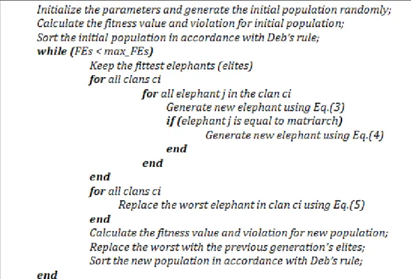
_maxare minimum and maximum bound in the search space.

The pseudo code of the basic EHO to solve the constrained optimization problem is given in Figure 1. By protecting the general structure of basic EHO, the adaptation of EHO algorithm is implemented with Deb’s rule to constrained optimization. Due to ease of implementation and an effective mechanism for the constrained optimization, the Deb’s rules are used as a constraint handling method in this study. In the Deb’s rule, there are rules on the selection between two solutions (Babalik et al., 2018; Deb, 2000):

1. When preferring between feasible and infeasible solution, feasible solution is directly selected. 2. If two solutions are feasible, better solution based in accordance with fitness value is selected. 3. If two solutions are infeasible, the solution with less violation is selected.

When the whole population is sorting, not only fitness values but also violations are considered. To apply the Deb’s rule, the population is sorting in accordance with violation values of elephants firstly, and then fitness values. Thus, if the violation values of two elephants are equal or zero, they are ranked according to their fitness value. If not equal, the elephant which has a higher violation value is worse than the elephant which has a lower violation value on the ranking.

Figure 1. The pseudo code of the basic EHO to solve constrained optimization problem

Due to the taking directly mean position of clan using a random number for updating the new position, Eq. (4) may causes the poor fit solution and inconsistency (Hakli, 2018; Parashar et al., 2017). As a cumulative effect, it undermines the process of finding the global best solution (Meena et al., 2018). Considering the discussion on the disadvantage of the Eq.(4), it is ignored in the new variant and this variant is named EHO-NoB. In my previous study (Hakli, 2018), a new EHO variant was proposed by balancing global and local search (GL-EHO). In the GL-EHO, the new search mechanism which is inspired by particle swarm optimization (PSO) (Kennedy and Eberhart, 1995) and artificial bee colony (ABC) (Karaboga, 2005) is used instead of the Eq.(3) in the basic EHO. These two EHO variants are adapted to constrained optimization as shown in Figure 1 except for the indicated changes.

EXPERIMENTAL RESULTS

The performance of algorithms is evaluated and investigated on the well-known 13 constrained optimization benchmark problems (Koziel and Michalewicz, 1999; Mezura-Montes and Coello, 2011; Runarsson and Yao, 2000). These problems are detailed in Appendix-A, and also you can find the details of these functions as a supplementary data in the Babalik et al.’s study (Babalik et al., 2018). G02, G03, G08 and G12 are maximization, and the other eights are minimization problems. In the experiments are performed in this study, the population size is 50, the number of elephant in each clan is set 10 and α is 0.5 for all EHO variants. For the basic EHO, β is determined as 0.1. The acceleration coefficients c1 and c2

are equal to each other and they are set 1.5 for the GL-EHO. To provide fair comparison, the maximum number of function evaluations is set 2.4E+5 as in other studies (Babalik et al., 2018; Ivana Strumberger et al., 2018), and the algorithms are run 30 times for each function.

The Experiments of EHO Variants

The experimental results of EHO variants for constrained optimization problem are given in Table 1. Table 1 contains the mean and standard deviation results of 30 runs for three EHO variants. In addition,

the optimum results of the problems are seen in Table 1. The best mean results obtained by algorithms for the benchmark problems are written as boldface.

Table 1. Experimental results of EHO variants for constrained optimization problems

Problem Min./Max. Optimal EHO EHO-NoB GL-EHO

G01 Min. -15,000 Mean -1,088 -14,500 -15,000 Std.Dev. 2,285 0,974 0,000 G02 Max. 0,803619 Mean 0,2522 0,4490 0,6405 Std.Dev. 0,018 0,020 0,069 G03 Max. 1,000 Mean 0,6560 0,4864 0,9026 Std.Dev. 0,088 0,250 0,360 G04 Min. -30665,539 Mean 30333,809 -30304,074 -30665,540 Std.Dev. 56,196 105,429 0,000 G05 Min. 5126,498 Mean 5373,189 5182,527 5502,522 Std.Dev. 174,591 69,539 406,900 G06 Min. -6961,814 Mean -6943,713 -6227,937 -6961,814 Std.Dev. 9,322 288,753 0,000 G07 Min. 24,306 Mean 446,6258 83,0228 36,9279 Std.Dev. 204,988 112,134 34,476 G08 Max. 0,095825 Mean 0,095376 0,095825 0,095825 Std.Dev. 0,000 0,000 0,000 G09 Min. 680,63 Mean 927,874 709,6519 681,7680 Std.Dev. 60,689 24,345 0,854 G10 Min. 7049,25 Mean 10236,025 8162,372 8374,642 Std.Dev. 677,597 1240,831 1481,337 G11 Min. 0,75 Mean 0,7400 0,7399 0,7399 Std.Dev. 0,000 0,000 0,000 G12 Max. 1,000 Mean 1,000 1,000 1,000 Std.Dev. 0,000 0,000 0,000 G13 Min. 0,05395 Mean 1,3335 1,0946 0,4043 Std.Dev. 1,056 0,858 0,213

When examining the Table 1, GL-EHO has better or same performance than the other variants on the eight problems. The basic EHO obtains the better solution than the other algorithm for only G11 function and it generally falls behind the EHO-NoB in terms of solution quality. This situation can be verified the discussion on the Eq.(4) of the basic EHO. The GL-EHO reaches optimal solution for G01, G04, G06, G08 and G12 problems and it outperforms the basic EHO and EHO-NoB in accordance with the experimental results are given in Table 1.

(a) (b)

(c) (d)

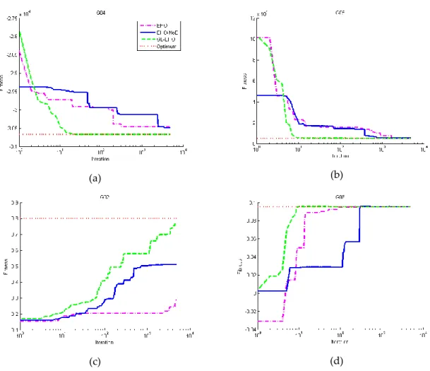
Figure 2. The convergence graphs of EHO variants

To analysis the convergence performances of EHO variants, convergence graphs of the methods are given in the Figure 2. In the Figure 2, there are four convergence graphs for the G04 (a) ,G05 (b), G02 (c) and G08 (d) problems. GL-EHO has a superior convergence performance and it reaches the optimum before basic EHO and EHO-NoB as seen in Figure 2. Although the basic EHO converges quickly than the EHO-NoB, it undergoes stagnation (especially G02) and EHO-NoB catches or gets ahead the basic EHO towards the end of the iteration.

A comparison of GL-EHO and other algorithms

The GL-EHO is more successful than the basic EHO and EHO-NoB in accordance with the results in the first experiment, so it is selected for comparison with other algorithms to validate its performance. The GL-EHO is compared with ABC, PSO, genetic algorithm (GA) and differential evolution algorithm (DE) and the experimental results of these algorithms given in Table 2 are directly taken from (Babalik et al., 2018).

Table 2. A comparison of GL-EHO and other algorithms

Problem Optimal ABC PSO GA DE GL-EHO

G01 -15,0000 Mean -15,0205 -10,5551 -14,2360 -14,2406 -15,0000 Difference 0,0205 4,4449 0,7640 0,7594 0,0000 G02 0,8036 Mean 0,4795 0,4043 0,7886 0,6660 0,6405 Difference 0,3241 0,3993 0,0150 0,1376 0,1631 G03 1,0000 Mean 3,0191 1,1675 0,9760 1,1694 0,9026 Difference 2,0191 0,1675 -0,0240 0,1694 -0,0974 G04 -30665,5390 Mean -30610,974 -30661,740 -30590,455 -30665,540 -30665,540 Difference 54,565 3,799 75,084 0,001 0,001 G05 5126,4970 Mean 5115,056 5298,284 N/A 5329,197 5502,522 Difference 11,441 171,787 N/A 202,700 376,025 G06 -6961,8140 Mean -7579,630 -6961,819 -6872,204 -6765,482 -6961,814 Difference 617,816 0,005 89,610 196,332 0,002 G07 24,3060 Mean 29,0956 28,7418 34,9800 24,3160 36,9279 Difference 4,7896 4,4358 10,6740 0,0100 12,6219 G08 0,0958 Mean 6,5347 0,0847 0,0958 0,0958 0,0958 Difference 6,4389 0,0111 0,0000 0,0000 0,0000 G09 680,6300 Mean 683,8941 680,7815 692,0640 680,6308 681,7680 Difference 3,2641 0,1515 11,4340 0,0008 1,1380 G10 7049,2500 Mean 7259,028 8128,793 10003,225 7162,592 8374,642 Difference 209,778 1079,543 2953,975 113,342 1325,392 G11 0,7500 Mean 0,7171 0,7626 0,7500 0,9545 0,7399 Difference 0,0329 0,0126 0,0000 0,2045 0,0101 G12 1,0000 Mean 1,0001 1,0000 1,0000 1,0000 1,0000 Difference 0,0001 0,0000 0,0000 0,0000 0,0000 G13 0,0955 Mean 0,0955 1,4228 N/A 0,9492 0,4043 Difference 0,0000 1,3273 N/A 0,8537 0,3088

Friedman Rank (Dif.) 3,46 3,12 3,35 2,58 2,50

Corrected Rank 5 3 4 2 1

The absolute difference values calculated by subtracting the mean values of the algorithms from the optimal values of the problems are presented in Table 2 so that the algorithms’ results can be evaluated clearly. Friedman rank test are implemented using absolute difference values of algorithms. With respect to the Friedman test, GL-EHO is first rank between the methods. In addition, the DE is second rank and ABC is located in the last rank.

A comparison of GL-EHO and other EHO variant on the constrained optimization

Strumberger et.al proposed a hybridized EHO (HEHO) for constrained optimization and they used a different approach for adaptation to constrained optimization (Ivana Strumberger et al., 2018). The limit parameter in the ABC algorithm was added to HEHO and when the generating new solution, the

Std.Dev. 0,012 0,000 G02 0,803619 Mean 0,799125 0,6405 Std.Dev. 0,026 0,069 G03 1,000 Mean 1,000 0,9026 Std.Dev. 0,000 0,360 G04 -30665,539 Mean -30499,033 -30665,540 Std.Dev. 16,302 0,000 G05 5126,498 Mean 5126,505 5502,522 Std.Dev. 0,041 406,900 G06 -6961,814 Mean -6957,361 -6961,814 Std.Dev. 1,005 0,000 G07 24,306 Mean 24,309 36,9279 Std.Dev. 0,003 34,476 G08 0,095825 Mean 0,095825 0,095825 Std.Dev. 0,000 0,000 G09 680,63 Mean 680,653 681,7680 Std.Dev. 0,011 0,854 G10 7049,25 Mean 7152,895 8374,642 Std.Dev. 95,239 1481,337 G11 0,75 Mean 0,751 0,7399 Std.Dev. 0,001 0,000 G12 1,000 Mean 1,000 1,0000 Std.Dev. 0,000 0,000 G13 0,05395 Mean 0,246 0,4043 Std.Dev. 0,106 0,213

As seen in the Table 3, while the GL-EHO has a better performance than the HEHO for G01, G04, G06 problems, it has a same performance with HEHO for G08 and G12. HEHO obtains the better result than the GL-EHO for the eight problems. Although the results of GL-EHO are comparable level with the results of HEHO, the HEHO approach is forefront on the constrained optimization by virtue of preventing the worse solutions. On the other hand, while the GL-EHO maintains the basic EHO characteristics except for the change of the search mechanism, the HEHO has more modifications on the basic EHO.

CONCLUSION

When solving the constrained optimization problems with the bio-inspired algorithms, these algorithms have been adapted to constrained optimization with some modifications using the constraint

handling methods. In this study, a new approach based on EHO algorithm was applied using Deb’s rules for constrained optimization. In addition, two EHO variants (EHO-NoB and GL-EHO) are adapted to constrained optimization with this new approach. The performances of these algorithms are evaluated on the well-known thirteen constrained optimization problems. The basic EHO has a weak performance due to the losing the diversification of population quickly. The GL-EHO outperforms the basic EHO and EHO-NoB by virtue of effective search mechanism. Moreover, GL-EHO has a better performance when comparing with other mostly known algorithms. The GL-EHO is compared with another EHO variant (HEHO) on the constrained optimization and its results are comparable level with the results of HEHO. Although, GL-EHO obtained the promising results by protecting the characteristic of basic EHO, it can be improved with some modifications or hybridized with other algorithms as a future work.

REFERENCES

Alihodzic, A., Tuba, E., Capor-Hrosik, R., Dolicanin, E., Tuba, M., 2017, "Unmanned Aerial Vehicle Path Planning Problem by Adjusted Elephant Herding Optimization", 2017 25th Telecommunication

Forum (Telfor), 804-807.

Asafuddoula, M., Ray, T., Sarker, R., 2014, "An adaptive hybrid differential evolution algorithm for single objective optimization", Applied Mathematics and Computation, 231, 601-618. doi:10.1016/j.amc.2014.01.041

Babalik, A., Cinar, A. C., Kiran, M. S., 2018, "A modification of tree-seed algorithm using Deb's rules for constrained optimization", Applied Soft Computing, 63, 289-305. doi:10.1016/j.asoc.2017.10.013 Deb, K., 2000, "An efficient constraint handling method for genetic algorithms", Computer Methods in

Applied Mechanics and Engineering, 186(2-4), 311-338. doi:Doi 10.1016/S0045-7825(99)00389-8

Farnad, B., Jafarian, A., Baleanu, D., 2018, "A new hybrid algorithm for continuous optimization problem", Applied Mathematical Modelling, 55, 652-673. doi:10.1016/j.apm.2017.10.001

Garg, H., 2016, "A hybrid PSO-GA algorithm for constrained optimization problems", Applied

Mathematics and Computation, 274, 292-305. doi:10.1016/j.amc.2015.11.001

Hakli, H., "An improved elephant herding optimization by balancing local and global search for continuous optimization", 15th International Conference on Informatics and Information

Technologies, CIIT 2018, Mavrovo, Macedonia. In Press. 2018.

Hakli, H., Uguz, H., 2017, "A novel approach for automated land partitioning using genetic algorithm",

Expert Systems with Applications, 82, 10-18. doi:10.1016/j.eswa.2017.03.067

Jiao, R. W., Zeng, S. Y., Alkasassbeh, J. S., Li, C. H., 2017, "Dynamic multi-objective evolutionary algorithms for single-objective optimization", Applied Soft Computing, 61, 793-805. doi:10.1016/j.asoc.2017.08.030

Karaboga, D., (2005). An idea based on honey bee swarm for numerical optimization. Retrieved from Technical Report-TR06, Erciyes University, Engineering Faculty, Comput. Eng.Dep.:

Kennedy, J., Eberhart, R., "Particle swarm optimization", Sixth International Symposium on Micro Machine

and Human Science, Nagoya,Japan. 39–43. 1995.

Kiran, M. S., 2015, "TSA: Tree-seed algorithm for continuous optimization", Expert Systems with

Applications, 42(19), 6686-6698. doi:10.1016/j.eswa.2015.04.055

Kohli, M., Arora, S., 2017, "Chaotic grey wolf optimization algorithm for constrained optimization problems", Journal of Computational Design and Engin eering, In Press.

doi:10.1016/j.jcde.2017.02.005

Koziel, S., Michalewicz, Z., 1999, "Evolutionary Algorithms, Homomorphous Mappings, and Constrained Parameter Optimization", Evolutionary Computation, 7(1), 19-44. doi:DOI 10.1162/evco.1999.7.1.19

Lin, C. H., 2013, "A rough penalty genetic algorithm for constrained optimization", Information Sciences,

Niu, B., Wang, J. W., Wang, H., 2015, "Bacterial-inspired algorithms for solving constrained optimization problems", Neurocomputing, 148, 54-62. doi:10.1016/j.neucom.2012.07.064

Parashar, S., Swarnkar, A., Niazi, K. R., Gupta, N., 2017, "A Modified Elephant Herding Optimization For Economic Generation Co-Ordination Of DERs And BESS In Grid Connected Microgrid",

Journal of Engineering-Joe.

Runarsson, T. P., Yao, X., 2000, "Stochastic ranking for constrained evolutionary optimization", Ieee

Transactions on Evolutionary Computation, 4(3), 284-294. doi:Doi 10.1109/4235.873238

Sambariya, D. K., Fagna, R., 2017, "A novel Elephant Herding Optimization based PID controller design for Load Frequency Control in Power System", 2017 International Conference on Computer,

Communications and Electronics (Comptelix), 595-600.

Sharma, A., Kumar, R., Panigrahi, B. K., Das, S., 2017, "Termite spatial correlation based particle swarm optimization for unconstrained optimization", Swarm and Evolutionary Computation, 33, 93-107. doi:10.1016/j.swevo.2016.11.001

Strumberger, I., Bacanin, N., Tomic, S., Beko, M., Tuba, M., 2017, "Static Drone Placement by Elephant Herding Optimization Algorithm", 2017 25th Telecommunication Forum (Telfor), 808-811.

Strumberger, I., Bacanin, N., Tuba, M., "Hybridized Elephant Herding Optimization Algorithm for Constrained Optimization", Cham. 158-166. 2018.

Tuba, E., Alihodzic, A., Tuba, M., 2017, "Multilevel Image Thresholding Using Elephant Herding Optimization Algorithm", 2017 14th International Conference on Engineering of Modern Electric

Systems (Emes), 240-243.

Wang, B.-C., Li, H.-X., Feng, Y., 2018, "An improved teaching-learning-based optimization for constrained evolutionary optimization", Information Sciences, 456, 131–144.

Wang, G. G., Deb, S., Coelho, L. D., 2015, "Elephant Herding Optimization", 2015 3rd International

Symposium on Computational and Business Intelligence (Iscbi 2015), 1-5. doi:10.1109/Iscbi.2015.8

Xu, B., Chen, X., Tao, L. L., 2018, "Differential evolution with adaptive trial vector generation strategy and cluster-replacement-based feasibility rule for constrained optimization", Information

Appendix A. Standard Constrained Optimization Problems G01 Problem 4 4 13 2 1 1 5 1 1 2 10 11 2 1 3 10 12 3 2 3 11 12 4 1 10 5 2 11 6 3 12 7 4 5 10 8 6 min ( ) 5 5 5 ( ) 2 2 10 0 ( ) 2 2 10 0 ( ) 2 2 10 0 ( ) 8 0 ( ) 8 0 ( ) 8 0 ( ) 2 0 ( ) 2 d d d d d d f x x x x subject to g x x x x x g x x x x x g x x x x x g x x x g x x x g x x x g x x x x g x x                                           







7 11 9 8 9 12 0 ( ) 2 0 0, 1, 2,...,13 1, 1, 2,...,9,13 i i x x g x x x x x i x i             G01

There are 13 decision variables and 9 constraint functions defined on the decision variables in G01 problem. The global minimum is -15 while decision variables are (1,1,…,1,3,3,3,1). The search space is

0

 

x

_i

u

_i

,

i



1, 2,...,

n and u



(1,1,...,1,100,100,100,1)

.

G02 Problem

subject to

There are 20 decision variables and 2 constraint functions defined on the decision variables in G02 problem. The global maximum is unknown, the best founded solution is 0.803619 (which, to the best of our knowledge, is better than any reported value), constraint is close to being active ( ).

There are 10 decision variables and a constraint function defined on the decision variables in G03 problem. The global maximum is 1, while decision variables are (i=1,…,n). The search space is

.

G04 Problem

subject to

There are 5 decision variables and 6 constraint functions defined on the decision variables in G04 problem. The global minimum is -30665.539 while decision variables are (78, 33, 29.995256025682, 45 and

36.775812905788). The search space is

, , , , .

G05 Problem

subject to

There are 4 decision variables and 5 constraint functions defined on the decision variables in G05 problem. The best known solution is 5126.4981 while decision variables are (679.9453, 1026.067,

0.1188764, -0.3962336). The search space

G06 Problem

subject to

There are 2 decision variables and 2 constraint functions defined on the decision variables in G06 problem. The optimum solution is -6961.81388 while decision variables are (14.095, 0.84296). The search

space is , .

G07 Problem

subject to

There are 10 decision variables and 8 constraint functions defined on the decision variables in G07 problem. The optimum solution is 24.3062091 while decision variables are (2.363683, 8.773926, 5.095984, 0.9906548, 1.430574, 1.321644, 9.828726, 8.280092, and 8.375927). The search space

is ,

G08 Problem

subject to

There are 2 decision variables and 2 constraint functions defined on the decision variables in G08 problem. The optimum solution is 0.095825 while decision variables are (1.2279713, 4.2453733). The

There are 7 decision variables and 4 constraint functions defined on the decision variables in G09 problem. The optimum solution is 680.6300573 while decision variables are (2.330499, 1.951372, -0.4775414, 4.365726, -0.6244870, 1.038131, and 1.594227). The search space

is ,

G10 Problem

subject to

There are 8 decision variables and 6 constraint functions defined on the decision variables in G10 problem. The optimum solution is 7049.3307 while decision variables are (579.3167, 1359.943, 5110.071,

182.0174, 295.5985, 217.9799, 286.4162, and 395.5979). The search space

is , , .

G11 Problem

subject to

There are 2 decision variables and a constraint functions defined on the decision variables in G11 problem. The optimum solution is 0.75 while decision variables are ( ). The search space

is and .

G12 Problem

There are 3 decision variables and a constraint functions defined on the decision variables in G12 problem. The feasible region of the search space consists of disjointed spheres. A point ( ) is feasible if and only if there exist p, q, r such that the above inequality holds. The optimum solution is 1 while decision variables are (5,5,5). The search space is and also p, q, r = 1, 2, …, 9. The solution lies within the feasible region.

G13 Problem

subject to

There are 5 decision variables and 3 constraint functions defined on the decision variables in G13 problem. The global minimum is 0.0539498 while decision variables are (1.717143, 1.595709, 1.827247,