© TÜBİTAK
doi:10.3906/elk-1911-79
h t t p : / / j o u r n a l s . t u b i t a k . g o v . t r / e l e k t r i k / Research Article
Accurate indoor positioning with ultra-wide band sensors
Taner ARSAN∗
Computer Engineering Department, Faculty of Engineering and Natural Sciences, Kadir Has University, İstanbul, Turkey
Received: 13.11.2019 • Accepted/Published Online: 28.01.2020 • Final Version: 28.03.2020
Abstract: Ultra-wide band is one of the emerging indoor positioning technologies. In the application phase, accuracy
and interference are important criteria of indoor positioning systems. Not only the method used in positioning, but also the algorithms used in improving the accuracy is a key factor. In this paper, we tried to eliminate the effects of off-set and noise in the data of the ultra-wide band sensor-based indoor positioning system. For this purpose, optimization algorithms and filters have been applied to the raw data, and the accuracy has been improved. A test bed with the dimensions of 7.35 m × 5.41 m and 50 cm × 50 cm grids has been selected, and a total of 27,000 measurements have been collected from 180 test points. The average positioning error of this test bed is calculated as 16.34 cm . Then, several combinations of algorithms are applied to raw data. The combination of Big Bang-Big Crunch algorithm for optimization, and then the Kalman Filter have yielded the most accurate results. Briefly, the average positioning error has been reduced from 16.34 cm to 7.43 cm .
Key words: Indoor positioning, ultra-wide band sensors, optimization, big bang-big crunch algorithm, genetic
algo-rithms, the Kalman filter
1. Introduction
We often use not only the outdoor positioning but also indoor positioning in our daily lives. Outdoor localization solutions have been improved over the years considering the Global Position System (GPS) and Assisted GPS technology. These solutions are highly effective in determining the position in outdoor areas. GPS is developed by the US Department of Defense and can best be described as a satellite based navigation system [1,2]. Outdoor positioning information can be calculated when four or more GPS satellites are within the field of view. GPS enables critical outdoor positioning, especially for civil, commercial and military applications. Assisted GPS (A-GPS) technology is a navigation system used on mobile devices that helps to identify a user’s location via the base station’s A-GPS address server [3]. The accuracy provided by the GPS in determining the outdoor location is between 3 m and 15 m , usually around 10 m . The accuracy that A-GPS provides in determining the outdoor location is about 15 m, while the interior is 50 m [3]. As can be seen from the accuracy values, these solutions are sufficient to determine the outdoor position, in other words, the position in the open space. On the other hand, given the fact that people now spend more than 80% of their time indoors, a suitable system for locating interior space is needed. Unfortunately, the use of GPS satellites in indoor location determination is not possible as GPS signals are weaken due to atmospheric delays, multi-paths, steel structures, roofs and building walls [1–3]. For this reason, efforts have been made to develop new technologies that allow reliable indoor location determination with high accuracy, low average positioning error over the past two decades. ∗Correspondence: [email protected]
However, new algorithms and methods are needed to improve the existing results. When the GPS signals cannot be reached, it is possible to use a different technology to determine the coordinates of indoor location by means of infrared, ultrasonic, cellular, radio frequency identification (RFID), wireless networks (Wi-Fi), Bluetooth Low Energy (BLE) beacons or Ultra-wide band (UWB) [4–6]. In some studies, even visible light has been used [7–9] as well as technologies that utilize the Earth’s magnetic field [10, 11]. Indoor positioning systems have been developed rapidly in recent decades. Methods of positioning are divided into two categories: the location fingerprint positioning method [12] and the trilateration algorithm [13]. The need for high accuracy indoor positioning is becoming a very important issue. Locating patients and workers in the hospital, finding employees in a large office and finding people trapped in a burning building are a few of the applications of indoor positioning systems that require high accuracy.
Many solutions have been developed for estimating the position of the indoor objects. Most of these solu-tions manage to provide locational information, and they are based on multi-lateration, and mostly triangulation methods using radio signals or infrared, and ultrasound. There are many indoor positioning systems (IPS) with different architectures, configurations, reliabilities, and accuracies to determine the location information of peo-ple and objects. In general, infrared (IR), Wi-Fi, RFID, BLE Beacon, ultrasonic and UWB are the technologies used in IPS [13,14]. One of the best solutions is to use Wi-Fi for indoor positioning. However, there are still several technical difficulties in the indoor localization based on Wi-Fi which have not been solved completely. The main problem is about indoor positioning accuracy. In [15], a method is developed to estimate the position of a tag. In this study, multi-lateration with probabilistic RFID map-based technique and the Kalman Filter is used together to improve the indoor positioning accuracy. As soon as this method is applied, more accurate position estimation and accelerations can be obtained. The bandwidth of Ultra-wide band (UWB) signals is extremely large, exceeding 500 MHz [16]. This offers many advantages for radar applications; and it improves reliability, since the signal contains different frequency components. Some of these frequency components can go through or around obstacles [17]. Thus, the UWB provides a more accurate and reliable positioning. The power consumptions of the UWB sensors are low when we compare them with localization technologies [18]. UWB offers a good multipath resolution, since the indoor wireless systems must cope with several multipath scenarios [19].
The geometric properties of triangles are used in the Triangulation method to estimate the position of a target. It includes two derivations: lateration and angulation. The lateration derivations estimate the location of an object by measuring its distances from more than one reference point. Received signal strengths (RSS) [20–22], the time of arrival (ToA) or time difference of arrival (TDoA) methods are usually used [23], instead of measuring the distance directly. In these methods, distance is calculated by computing the attenuation of the emitted signal strength or by multiplying the travel time and radio signal velocity. Roundtrip time of flight (RToF) method is also used for range estimation in some systems whereas Angulation locates an object by computing angles relative to multiple reference points in Angle of Arrival (AoA) method [24].
UWB is promising in indoor environments because it has nonprone to interference behavior, and much better penetrating capability [25–27]. However, the location accuracy can be affected by the presence of a line-of-sight (LoS) obstruction for two reasons. Firstly, there is excess propagation delay because of the high level of dielectric constant of the LoS blocking material. This may cause bias in the location estimation. Secondly, the propagation channel has multipath structure, and it has a complex behavior. The more complex the behavior, the more difficult it is to estimate the time of arrival (ToA) from the direct path signal [25–27].
1.1. Related previous works
Before the MDEK10011UWB sensors that were the main subject of this study, indoor positioning studies [28]
were performed by using Wi-Fi, BLE beacons and TREK10002UWB sensors. The aim of these studies was to
minimize the average positioning error value as much as possible [28]. The results obtained from the studies in approximately 36 m2 test areas reduced average positioning error values of 139 cm with Wi-Fi technology, 86 cm with BLE Beacon technology, and 24 cm with TREK1000 UWB sensors [28]. These results show that indoor positioning method can be applied to behavior mapping [28]. As a matter of fact, if only manual behavior mapping is possible with an average positioning error value of less than 20 cm, it may be possible to perform behavior mapping automatically by determining the user’s indoor location. Therefore, the studies shifted in this direction. The average positioning error value of 24 cm was first reduced to 20.72 cm by making the necessary calibrations and developing a ceiling system by placing UWB sensors at the appropriate height [29]. These studies are still being carried out on a multi-disciplinary platform. The most important development, currently needed, is to be able to calculate both behavior mapping and interaction between users by minimizing the average positioning error value. The first study to this end is to reduce two fundamental errors, especially during measurement. Although the first error source was meticulously studied and calibrated as required, an offset value was generated during the measurement. The second source of error is the noise effect caused by disturbances and reflections. TREK1000 UWB sensors were used in the first studies to eliminate the offset value and all the results were tested by calculating a common offset value. In [29], a single offset value was obtained. By using this offset value, it was possible to reduce the average positioning error value from 20.72 cm to 15.02
cm [29]. Afterwards, the studies have been developed to reduce offset and noise effects in order to reduce the average positioning error to around 15 cm.
1.2. The main contribution
This work provides a potential application of behavior mapping with multiple UWB sensors by reducing the average positioning error by less than 8 cm. Briefly, the aim of this article is to find a proper solution to obtain improved accuracy of MDEK1001 UWB sensor-based IPS to reduce the average positioning error value to less than 8 cm, as it is currently around 16 cm to 20 cm. For this purpose, all the combinations of BB-BC algorithm, genetic algorithm and the Kalman Filter are examined and implemented in an active learning classroom (ALC) test bed. The accuracy of indoor positioning is increased further, and preliminary studies are conducted to understand the interaction of two or more users with individual movements, such as swinging left and right, and multiple users in behavior mapping, which will enable future studies.
The contribution of this work is threefold:
• Eliminating the offset value that affects the raw data accuracy, it is also called bias cancellation. We use the BB–BC optimization algorithm and the genetic algorithm to achieve this aim.
• Removing outliers and noise caused by interference. We use the Kalman Filter to achieve this aim. • Finding the exact order of the methods which provides a better accuracy, briefly low average positioning error to less than 8 cm. This also allows multiple users of behavior mapping.
The organization of the rest of the article is as follows: Section 2 introduces all the proposed methods; BB-BC optimization algorithm, genetic algorithm and the Kalman Filter are explained in detail. Section 3 1MDEK1001 (2017). MDEK1001 Kit User Manual Module Development and Evaluation Kit for the DWM1001 [online]. Website https://www.decawave.com/mdek1001/usermanual/ [accessed 8 June 2019]. DecaWave (2017).
2TREK1000 (2016): TREK1000 User Manual, How to Install, Configure and Evaluate the Decawave Trek1000 Two-Way Ranging (TWR) RTLS IC Evaluation Kit. Website https://www.decawave.com/trek1000/usermanual [accessed 22 May 2019]. DecaWave (2016).
describes experimental setup and indoor positioning dataset. Section 4 introduces experimental studies and results. While BB-BC or GA is used for removing the offset value dataset, the Kalman Filter is used for noise cancellation. In this section, combinations of optimization algorithm and filtering is experimentally applied. Section 5 presents the discussion about the accuracy results that we have obtained from all the applied methods. Our paper is completed by the conclusions in Section 6.
2. The proposed methods
The proposed methods are the Big Bang-Big Crunch (BB-BC) optimization algorithm [30,31] and the Genetic Algorithm [32–34] for eliminating the offset value (bias cancellation) and optimization, the Kalman Filter [35–37] for removing outliers and noise caused by interference:
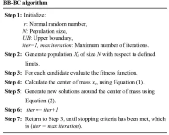
2.1. The big bang-big crunch algorithm (BB-BC)
The BB-BC algorithm essentially consists of two stages: a big bang (BB) stage and a big crunch (BC) stage. In BB stage, candidate solutions will be distributed uniformly over the search space. The BC stage can be visualized as a transformation from a disordered state of energy to an ordered state of energy. The BC has multiple inputs, and one output, namely, center of ‘mass’. The BC is a concurrence operator, and the word ‘mass’ indicates the inverse of the objective function value. The center of mass is calculated as follows [30,31]:
− →xc= N ∑ i=1 − →xi fi N ∑ i=1 1 fi , (1) where −→xi, f
i , N denote a point within an n -dimensional search space, the objective function value for this
point, and population size, respectively. After the BC stage, the optimization algorithm creates new members to be used for the BB stage in the next iteration. This process can be achieved by jumping to the first step and generating an initial population.
For an optimization algorithm to be classified as global, it must converge to an optimal point. For this, it must include certain points that have a decreasing probability within its search population. So, a large number of solutions produced must be around the optimal point, and only few remaining points are distributed within the search space after a fixed number of steps. As the number of iterations increases, the ratio of solution points around the optimal value to points away from optimal value must decrease. The center of mass can be utilized by spreading new offsprings around it. After that, the center of mass will be recomputed. These contraction steps are performed until a specified stopping rule. The new candidates around the center of mass are then calculated as [30, 31]:
xnew= xc+L γ
k , (2)
where xc, γ , L , k represent center of mass, normal random number, the upper bounds on the values of the
optimization problem variables, and the iteration step respectively. As the number of iterations approaches infinity, the deviation term will reach zero. Hence, there will always be offsprings located far from the center
of mass with decreasing probability, but will never equal zero. This will assure the global convergence of the algorithm. The pseudocode of BB-BC algorithm is given in Figure 1.
Figure 1. Pseudocode of big bang-big crunch algorithm.
2.2. The genetic algorithm (GA)
The GA is a heuristic algorithm that can be applied in a straightforward manner and implemented in a wide variety of problems. Due to its population characteristics, the GA has been extended to solve search and optimization problems efficiently, including multi-objective and multimodal ones [32]. GA is based on genetics and biological evolution in which design variables are represented as genes on a chromosome. It features a group of candidate individuals called population on the response surface. Because of its genetic operators and environmental selection, mutation and recombination, chromosomes that have an optimal fitness are obtained [32].
Genetic algorithm was invented by ”John Holland” in the 1960s, and consists of the following four important steps [34]:
(i) Initial candidate population of chromosomes are formed in two ways: (i) randomly, (ii) by perturbing an input chromosome. The way the initialization step is done is not critical if the initial population extends into a wide range of design variable settings. Hence, if there is information about the system optimization, this information can be adopted in the initial population. In the binary representation, every chromosome is a string of zeros or ones and the length of the string depends on the required accuracy.
(ii) Evaluation of the fitness is computed at this step. The fitness function aims to numerically encode the performance of the chromosome. In real world applications, the selection of the fitness function is considered a critical step.
(iii) Then, the chromosomes with the highest scores when it comes to the fitness are placed once or several times into a mating pool subset. This placement is in a semi-random manner. The low fitness chromosomes are removed from the population.
(iv) Exploration includes the crossover and mutation operators. Two chromosomes are selected randomly from the mating pool subset to be mated. The probability that these parents are mated is usually initialized
with a high value, and its user-controlled option. If the parent chromosomes can mate, a crossover operator is utilized to exchange the genes between the two parents to output two offspring. If they cannot mate, the parents are copied into the next generation unchanged. The pseudocode of Genetic Algorithm is given in Figure 2.
Input: nP: Population size, nVar: Number of variables, Initial population range, mG: Maximum generation. Output: The best individual in all generation.
Step 1: Generate initial population of size nP.
while (Number of generations is less than mG) Step 2: evaluate the initial population according to
the fitness function.
Step 3: select the individual according to their
fitness (selection).
Step 4: do crossover with Pc probability. Step 5: do mutation with Pm probability. Step 6: update population (population=selected
individual after Step 4 and 5).
end while
Step 7: Return the best individual. Genetic algorithm
Figure 2. Pseudocode of genetic algorithm.
2.3. The kalman filter (KF)
The Kalman Filter (KF) algorithm uses a serial data, which may contain noise, and is observed over time. The main goal is to increase the accuracy in estimation of the unknown variables [35]. The KF was proposed firstly by Rudolf Emil Kálmán in 1960 [38], and it became a standard approach to achieve optimal estimation. The KF is considered as one of the most famous Bayesian filter theories [36]. The state equation and observation equation are the linear representation of wk, uk, x(k−1) and xk, vk, and they represent a dynamic model in
the reliable estimation corrected by measurements [8]. The state equation of the Kalman Filter is represented as follows [35]:
xk = F xk−1+ B uk+ wk, (3)
whereas the observation equation is represented as follows:
zk = H xk+ vk, (4)
where in the above equations: F , xk, H , wk, zk, vk, uk represent the state transition matrix, state vector,
observation matrix, system noise vector, observation vector, observation noise vector, and system control vector, respectively. wk and vk are assumed to satisfy positive definite, uncorrelated and symmetric, zero mean white
Gaussian noise vector.
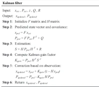
The pseudocode of the KF is given in Figure 3. In Figure 3, xest, Pest, z , R , Q are the predicted
state estimate vector, estimate covariance matrix, observation matrix, covariance matrix of the measurement noise, and the covariance of the process noise, respectively. xupdated and Pupdated represent fully parameterized
considered as follows. There is no variance or standard deviation used for the Kalman Filter implementation.
H is a combination of 1’s and 0’s , since the state of a system that we apply a Kalman Filter to is directly
measurable. H transforms the current estimate of state to the best estimate of the system output zk. F is set
to an identity matrix, used for updating the last-known estimate of state, xk−1 to reflect the current state at
xk. Input matrix B is set to zero, so no system input (control) is used as an input to the Kalman Filter.
Figure 3. Pseudocode of the kalman filter.
3. Experimental setup and indoor positioning data
In this article, we use a dataset taken from a 39.76 m2 ACL, measuring 7.35 m × 5.41 m. Some desks, chairs and moveable tables are available in the classroom, as shown in Figure 4. It is easy to provide several seating alternatives. The class is limited to 28 people; and it is designed to provide maximum control for the users [28]. The 12 people setup is used when the dataset is collected, as in Figure 4. While the ACL is designed as a test bed for collecting data, the anchors are attached to the ceiling (shown as A0, A1, A2 and A3 in Figure 4), and they are held on each corner of the testbed at 2.85 m height.
Decawave MDEK 1001 UWB development kit is used in this experiment by including 4 anchors in the ceiling and a tag for a test user. MDEK 1001 development kit contains 12 sensors, which are configurable as 1 to 8 tags and 4 to 11 anchors. For 39.76 m2 test bed, 4 anchors are convenient, but if we consider around 100
m2 test bed, it is possible to use up to 11 anchors for 1 kit, and up to 30 anchors for 3 kits to cover the area. In this condition, a tag can select the most convenient anchors dynamically as it passes through the area. The future studies will be conducted on multiple sensors and a larger test bed. As shown in Figure 5, an adaptive, remotely controlled ceiling system is developed to offer better LOS and also a direct path between the anchors and the tag. In the test area, the measuring points are marked at every 50 cm starting from (0, 0). In this way, a total of 180 test points are identified. The test user, wearing a UWB sensor called tag around the neck area, collects the location data of the test user. A total of 150 measurements are taken from each point; and the total number of measurements is 27,000; the duration of data collection is around 9 hours. The total time does not include the change of observation cycles and the time for set-up.
Figure 4. Layout of the active learning classroom; the dimension is 7.35 m × 5.41 m, A0, A1, A2 and A3 are the anchors, Tag1 is the tag for the test user, × denotes the test points, and the grid size is 50 cm × 50 cm.
Decawave MDEK 1001 UWB development kit contains single chip CMOS Ultra-Wideband integrated circuit, which supports the IEEE 802.15.4–2011 UWB standard. It operates at data rates of 6.8 M bps in 30 m range. It also uses UWB Channel 5 with 6.5 GHz and supports up to 10 Hz update rate for each individual tag and up to 150 updates per second per cluster. MDEK1001 supports a wide range of applications in fields as varied as engineering, healthcare, defense, shipping, logistics and inventory management systems for real time indoor positioning systems.
A0 A1
A2
A3
Figure 5. Adaptive ceiling system; four Decawave MDEK1001 UWB sensors (anchors) are mentioned as A0, A1, A2
and A3.
4. Experimental studies and results
The experiments and evaluation studies are carried out using the active learning classroom data set. The goal is to improve the accuracy of UWB sensor-based IPS by applying two optimization algorithms; namely, BB-BC and GA. When it comes to the performance metrics, the accuracy provided by the two algorithms are used as the comparison metric between the implemented algorithms. The accuracy is the Euclidean distance between the measured location to real location for each point [39]:
d =√(xr− xm)2+ (yr− ym)2, (5)
where ( xr, yr) are the coordinates of real location and ( xm, ym) are the coordinates of the measured location.
The active learning classroom dataset has 180 test points location. At each location, the test user collects 150 samples. The dataset is randomly divided into two sets: the training set and the test set. 105 of the samples (70%) are for the training set, and 45 of the samples (30%) are for the test set.
4.1. Stand-alone BB-BC and GA implementation
In population-based approaches, the fitness function value is evaluated for every candidate solution in each population. Thus, it has a major impact on the algorithm’s speed. The proposed system flow chart for BB-BC algorithm is shown in Figure 6, whereas the proposed system for GA is shown in Figure 7. The fitness function
in both algorithms are given as : Fm,r= N ∑ i=1 [
(Xim− Xiof f set− Xir)2+ (Yim− Yiof f set− Yir)2
]
, (6)
values are presented by Xiof f set, Yiof f set, whereas Xim and Yim represent the measured UWB values. The
population size is set to 100; and the number of generations is 500, which also refers to the maximum number of iterations that acts as stopping criteria for the proposed system for both the BB-BC and GA. In GA, the crossover probability is 0.8, whereas the probability of mutation is 0.1. In the first implementation, the system is trained using the raw UWB test points as an input to the proposed systems as shown in Figure 6 and Figure 7. As a result, for every test point (180 test points), the Xof f set and Yof f set values are obtained. In order to
apply these offset values to the test set, the average for each test point (XAvg, YAvg) in both the training set
and the test set are calculated. Then, the average of test point (XAvg, YAvg) in the test set that has the nearest
distance to the test point (XAvg, YAvg) in the training set uses the corresponding (Xof f set, Yof f set) value. The
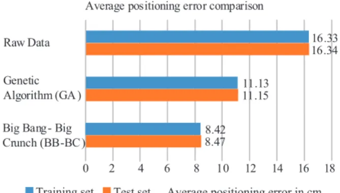
average localization error comparison of the BB-BC and GA is shown in Figure 8.
The time consumption for big bang - big crunch and genetic algorithms in experimental studies for a total of 180 locations, and 150 samples for each marked location are as follows. For genetic algorithm, the total time consumption is 1300.90 s; for big bang - big crunch algorithm, it is 560.90 s. The BB-BC algorithm has smaller time consumption, since GA has slow convergence when reaching the optimal result as compared to BB-BC.
4.2. BB-BC and GA with the kalman filter
In order to obtain better results and improve the effect of the optimization algorithms, the Kalman Filter is used in the second implementation on ALC data set. Since filtering the noise in signals is important, this comes from the fact that many sensors have an output that is too noisy to be used directly, and the Kalman Filter removes the uncertainty in the signal considered.
In order to compare the effect of using the Kalman Filter, two scenarios are performed. In the first scenario, the Kalman filtered UWB test points are used as an input to the proposed system, instead of the raw UWB measurements. The average positioning error comparison of the implemented algorithms for the first scenario are shown in Figure 9. In the second scenario, the raw UWB test points are used as input to the proposed systems. Then, the Kalman Filter is applied to the output data. The improvement in the average positioning error for the test set when performing BB-BC and GA is shown in Figure 10 and Figure 11, respectively. Figure 12 shows the comparison in the average positioning error for the second scenario, in which the results are significantly improved compared to the first scenario. The average positioning error comparison for all the implemented scenarios when performing BB-BC and GA are presented in Figure 13.
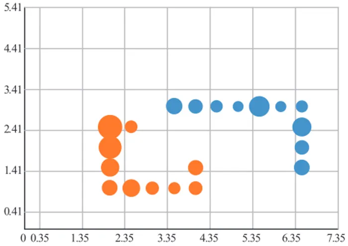
Finally, the moving sensor path location traces for two tags; blue tag and orange tag are given in Figure 14 and Figure 15. Here, the blue tag starting from (6.5,1.5) coordinates and stops at each test point by taking measurements to the left of the (6.5,3.0) coordinates; and has reached the point (3.5,3.5). The blue tag, starting from (4.0,1.5), proceeded by turning right three times, and stopped at each test point, reaching the point (2.5,2.5). Measurements were taken at 10 test points for both tags. Figure 14 shows the results for raw data; and Figure 15 shows the results for BB-BC then KF. The diameter of the circle is proportional to the average positioning error value. The average positioning error value for raw data was 16.51 cm and 7.51 cm for BB-BC then KF. The improvement was 54.51%. This result is important in terms of showing the accuracy of the study.
Input Test Points Tsi (i=1,…,180) Randomly select 30% for test Randomly select 70% for training Calculate average values XAvg and YAvg
Calculate average values XAvg and YAvg
Ts1=(Xim-Xof fset), (Yim-Yof fset)
Ts2=(Xim-Xof fset), (Yim-Yof fset)
.
Ts180=(Xim-Xof fset), (Yim-Yof fset)
Compare XAvg and YAvg
from two sources based on distance
Form an initial generation of N candidates in a random manner. Respect the limits of
the search space Calculate the Fitness
Function of Fm,r End Start Calculate new candidates around the center of mass:
xne w
Stopping Criteria? YES
NO
Ts1(XAvg-YAvg): (Xof fset-Yof fset)
Ts2(XAvg-YAvg): (Xof fset-Yof fset) .
Ts180(XAvg-YAvg): (Xof fset-Yof fset)
Calculate the Center of Mass
xc
Figure 6. Flow chart for proposed BB-BC optimization
method.
Input Test Points Tsi (i=1,…,180) Randomly select 30% for test Randomly select 70% for training Calculate average values XAvg and YAvg
Calculate average values XAvg and YAvg
Ts1=(Xim-Xof fset), (Yim-Yof fset)
Ts2=(Xim-Xof fset), (Yim-Yof fset)
.
Ts180=(Xim-Xof fset), (Yim-Yof fset)
Compare XAvg and YAvg
from two sources based on distance
Form an initial generation of N candidates in a random manner. Respect
the limits of the search space End Start Stopping Criteria? YES NO
Ts1(XAvg-YAvg): (Xof fset-Yof fset)
Ts2(XAvg-YAvg): (Xof fset-Yof fset)
.
Ts180(XAvg-YAvg): (Xof fset-Yof fset)
Evaluate the initial population according to
the Fitness Function of Fm,r
Selection
Crossover
Mutation
Figure 7. Flow chart for proposed Genetic Algorithm.
Average positioning error comparison
Raw Data 16.33
16.34
Average positioning error in cm Training set Test set
0 2 4 6 8 10 12 14 16 18 Genetic
Algorithm (GA )
11.13 11.15 Big Bang - Big
Crunch (BB-BC )
8.42 8.47
Figure 8. The average positioning error comparison,when
applying the raw UWB measurement as an input.
Average positioning error comparison
Raw Data 16.3316.34 0 2 4 6 8 10 12 14 16 18 11.23 11.27 Kalman Filtered (KF ) KF then GA KF then BB -BC 8.69 8.73 7.91 7.96
Average positioning error in cm Training set Test set
Figure 9. The average positioning error comparison, when applying the Kalman Filtered UWB measurement as an input.
BB - BC then KF Test Points 1 60 120 180 A v er ag e p o si ti o n in g e rr or i n m 0 .45 0 .40 0 .35 0 .30 0 .25 0 .20 0 .15 0 .10 0 .05 0
Raw Data BB -BC then KF
Figure 10. Average positioning errors of BB-BC when
applying the Kalman Filtered UWB measurement as an input. GA then KF A v er ag e p o si ti o n in g e rr o r in m 0.45 0.40 0.35 0.30 0.25 0.20 0.15 0.10 0.05 0 Test Points 1 60 120 180 Raw Data GA then KF
Figure 11. Average positioning errors of GA when
apply-ing the Kalman Filtered UWB measurement as an input.
Average positioning error comparison
Average positioning error in cm Raw Data
Kalman Filtered (KF)
GA then KF
BB-BC then KF
Training set Test set
0 2 4 6 8 10 12 14 16 18 16.33 16.34 11.23 11.27 7.82 7.83 7.37 7.43
Figure 12. The comparison of average positioning errors
when applying the Kalman Filtered UWB measurement as an input.
Genetic Algorithm -GA
Average positioning error comparison Raw Data Kalman Filtered -KF KF then GA BB-BC KF then BB -BC GA then KF BB-BC then KF
Average positioning error in cm 0 5 10 15 20 16.34 11 .27 11.15 8.73 8.47 7.96 7.83 7.43
Figure 13. The comparison of average positioning errors
for all implemented simulations.
5. Discussion
In this research article, BB-BC optimization algorithm and Genetic Algorithm are used to eliminate the offset value of UWB sensor measurements. The Kalman Filter is used to reduce the noise effect. As a result of these studies, BB-BC optimization method is applied to raw data to further improve the average positioning error value calculated with raw data as 16.34 cm. The offset value is calculated at each point; and the average positioning error value is found to be 8.47 cm. Genetic algorithm is then used; and the average positioning error value is 11.15 cm. Finally, only the Kalman Filter method is applied; and the mean error value is 11.27
cm . At this point, the most successful result is obtained with BB-BC algorithm. From this point on, the studies
are developed on which, firstly, the offset and noise effects are eliminated. Combinations of BB-BC and Genetic Algorithms are used for offset solution, and the Kalman Filter is used for noise reduction. Accordingly, the average positioning error value is 7.83 cm when first Genetic Algorithm, and then the KF is applied; 8.73 cm when first the KF, then Genetic Algorithm is applied; 7.43 cm when first BB-BC, then the KF is applied; 7.96
0 0.35 1.35 2.35 3.35 4.35 5.35 6.35 7.35 5.41 4.41 3.41 2.41 1.41 0.41
Figure 14. The comparison of moving sensors related to
Raw Data. 0 0.35 1.35 2.35 3.35 4.35 5.35 6.35 7.35 5.41 4.41 3.41 2.41 1.41 0.41
Figure 15. The comparison of moving sensors related to
BB-BC then KF Data.
of algorithms to improve the offset value and then the noise effect yields more accurate results; and the best average positioning error value is obtained as 7.43 cm when BB-BC then the KF is applied. As a result, the target of reducing the average positioning error value to less than 8 cm is achieved. These obtained results are better than newly developed systems such as [40]; and seem to be a good alternative for indoor positioning. Future research direction would be to apply BB-BC, then the KF method to multiple UWB sensors based indoor positioning system.
6. Conclusions
In this article, two optimization methods are compared in terms of accuracy using the ALC dataset, namely, Big Bang-Big Crunch (BB-BC) optimization algorithm and Genetic Algorithm (GA). In conclusion, the BB-BC outperforms GA during the implementations carried out in this study.
In the first implementation, the raw UWB measurements are used as an input to the proposed systems for BB-BC and GA. The obtained results prove that the reduction of average positioning error is from 16.34 cm to 8.47 cm; the improvement is around 48.16%, when applying BB-BC algorithm. The GA manages to reduce the average positioning error from 16.34 cm to 11.15 cm ,the improvement is only 31.76%.
In the second implementation, the Kalman Filtered UWB measurements are used as an input to the proposed systems. The results of this implementation show that the BB-BC algorithm is better in than the GA, in which the average positioning error is from 16.34 cm to 7.96 cm, the improvement is 51.29%, when applying BB-BC while the GA reduces the average positioning error from 16.34 cm to 8.73 cm, and the improvement is 46.57%.
During the second simulation, another scenario is performed in which the raw UWB measurements are used as an input to the proposed systems. Then, the optimized UWB measurements are used as an input to the Kalman Filter. The best results are acquired in this study from the implementation of this scenario. The GA algorithm, and then the KF method reduced the average positioning error by approximately 52.08%, from 16.34 cm to 7.83 cm, whereas the BB-BC algorithm, and then the KF method is able to reduce the average positioning error by approximately 54.53%, from 16.34 cm to 7.43 cm. Briefly, BB-BC, and then the KF method gives the best results in this research study.
When it comes to the limitation of GA, it is noticed that GA has slow convergence when reaching the optimal result; the optimal results in this case are the optimal offset values. This drawback is overcomed by the BB-BC algorithm, since it yields convergence rapidly when approaching the optimal value.
As mentioned in the main contribution section, this study presents a potential application of behavior mapping with multiple UWB sensors by reducing the average positioning error by less than 8 cm. We can clearly observe that we can obtain an average positioning error of 7.43 cm when applying BB-BC, and then KF to the raw data. This is the most important necessary condition for multi-sensor behavior mapping; and it is already satisfied. Future studies will be carried on the multi-sensor behavior mapping with newly developed real-time location system software in a larger test bed.
Acknowledgments
The author would like to thank Kadir Has University for financially supporting this research under grant number 2017-BAP-09. The author wishes to thank Associate Professor Osman Kaan Erol, the inventor of Big Bang-Big Crunch Algorithm, for his valuable comments and encouragements. The author also thanks Mr. Mohammed Muwafaq Noori Hameez, who was an M.Sc. student of the author, for his technical support with the experiments.
References
[1] Kaplan E, Hegarty C. Understanding GPS: Principles and Applications. Norwood, MA, USA: Artech House, 2008. [2] Hofmann-Wellenhof B, Lichtenegger H, Collins J. Global Positioning System: Theory and Practice. Wien, Austria:
Springer, 2001.
[3] Djuknic GM, Richton RE. Geolocation and assisted GPS. Computer 2001; 34(2): 123-125. doi: 10.1109/2.901174 [4] Huang H, Gartner G. A Survey of mobile indoor navigation systems. In: Gartner G, Ortag F (Editors). Cartography
in Central and Eastern Europe. Springer: Heidelberg, Germany, 2010, 305-319.
[5] Liu H, Darabi H, Banerjee P, Liu J. Survey of wireless indoor positioning techniques and systems. IEEE Trans-actions on Systems, Man, and Cybernetics, Part C Applications and Reviews 2007; 37 (6): 1067-1080. doi: 10.1109/TSMCC.2007.905750
[6] Gu YY, Lo A, Niemegeers I. A survey of indoor positioning systems for wireless personal networks. IEEE Commu-nications Surveys and Tutorials 2009; 11 (1): 13-32. doi: 10.1109/SURV.2009.090103
[7] Ganick A, Ryan D. Method and system for modulating a light source in a light based positioning system using a DC bias. US Patent 2012; Patent No: US 8,334,901 B1.
[8] Komine T, Nakagawa M. Fundamental analysis for visible-light communication system using LED lights. IEEE Transactions on Consumer Electronics 2004; 50 (1): 100-107. doi: 10.1109/TCE.2004.1277847
[9] Kumar N, Lourenco N, Spiez M, Aguiar R. Visible light communication systems conception and VIDAS. IETE Technical Review 2008; 25 (6): 359-367. doi: 10.4103/0256-4602.45428
[10] Shao WH, Zhao F, Wang C, Luo HY, Zahid TM et al. Location fingerprint extraction for magnetic field magnitude based indoor positioning. Journal of Sensors 2016; 1-16. doi: 10.1155/2016/1945695
[11] Galván-Tejada CE, García-Vázquez JP, Brena RF. Magnetic field feature extraction and selection for indoor location estimation. Sensors 2014; 14 (6): 11001-11015. doi: 10.3390/s140611001
[12] Gu Y, Chen M, Ren F, Li J. HED: Handling environmental dynamics in indoor WiFi fingerprint localization. In: Proceedings of the IEEE Wireless Communications and Networking Conference (WCNC); Doha, Qatar, 3-6 April 2016. pp. 1-6.
[13] Brena RF, García-Vázquez JP, Galván-Tejada CE, Muñoz-Rodriguez D, Vargas-Rosales C et al. Evolution of indoor positioning technologies: A survey, Journal of Sensors 2017; 1-21. doi: 10.1155/2017/2630413
[14] Gezici S. A survey on wireless position estimation, Wireless Personal Communications 2008; 44 (3): 263-282. doi: 10.1007/s11277-007-9375-z
[15] Bekkali A, Sanson H, Matsumoto M. RFID Indoor positioning based on probabilistic RFID map and Kalman filter-ing. In: Third IEEE International Conference on Wireless and Mobile Computing, Networking and Communications (WiMob 2007); White Plains, NY; 2007. pp. 1-7.
[16] Fort A, Ryckaert J, Desset C, De Doncker P, Wambacq P, Van Biesen L. Ultra-wideband channel model for communication around the human body. IEEE Journal on Selected Areas in Communications 2006; 24 (4): 927-933. doi: 10.1109/JSAC.2005.863885
[17] Hämäläinen M, Hovinen V, Latva-aho M. Survey to ultra-wide band systems. In: European Cooperation in the Field of Scientific and Technical Research–COST 262; Thessaloniki, Greece; 1999.
[18] Kopta V, Farserotu J, Enz C. FM-UWB: Towards a robust, low-power radio for body area networks. Sensors 2017; 17 (5): 1043-1063. doi: 10.3390/s17051043
[19] De Santis V, Feliziani M, Maradei F. Safety assessment of UWB radio systems for body area network by the (FDTD)-T-2 method. IEEE Transactions on Magnetics 2010; 46 (8): 3245-3248. doi: 10.1109/TMAG.2010.2046478 [20] Lee B, Lee Y, Chung W. 3D Navigation real time RSSI-based indoor tracking application. Journal of Ubiquitous
Convergence Technology 2008; 2 (2): 67-77.
[21] Dag T, Arsan T. Received signal strength based least squares lateration algorithm for indoor localization. Computers and Electrical Engineering 2018; 66: 114-126. doi: 10.1016/j.compeleceng.2017.08.014
[22] Kumar P, Reddy L, Varma S. Distance measurement and error estimation scheme for RSSI based localization in wireless sensor networks. In: Proceedings of the 5th IEEE Conference on Wireless Communication and Sensor Networks (WCSN); Allahabad, India; 2009. pp. 1-4.
[23] Dardari D, Conti A, Ferner U, Giorgetti A, Win MZ. Ranging with ultrawide bandwidth signals in multipath environments. Proceedings of the IEEE 2009; 97 (2): 404-426. doi: 10.1109/JPROC.2008.2008846
[24] Mahfouz M, Kuhn M, Wang Y, Turnmire J, Fathy A. Towards sub-millimeter accuracy in UWB positioning for indoor medical environments. In: Proceedings of the 2011 IEEE Topical Conference on Biomedical Wireless Technologies, Networks, and Sensing Systems (BioWireleSS); Phoenix, AZ, USA; 2011.
[25] Alarifi A, Al-Salman A, Alsaleh M, Alnafessah A, Al-Hadhrami S et al. Ultra wideband indoor positioning tech-nologies: Analysis and recent advances. Sensors 2016; 16 (5): 707. doi: 10.3390/s16050707
[26] Gigl T, Janssen GJM, Dizdarevic V, Witrisal K, Irahhauten Z. Analysis of a UWB indoor positioning system based on received signal strength. In: 4th Workshop on Positioning, Navigation and Communication; Hannover, Germany; 2007. pp. 97-101.
[27] Gezici S, Tian Z, Giannakis GB, Kobayashi H, Molisch AF et al. Localization via ultra-wideband radios. IEEE Signal Processing Magazine 2005; 22 (4): 70-84. doi: 10.1109/MSP.2005.1458289
[28] Arsan T, Kepez O. Early steps in automated behavior mapping via indoor sensors. Sensors 2017; 17 (12): 2925, 1-22. doi: 10.3390/s17122925
[29] Arsan T. Improvement of indoor positioning accuracy of ultra-wide band sensors by using big bang-big crunch op-timization method. Pamukkale University Journal of Engineering Sciences 2018; 24 (5): 921-928. doi: 10.5505/pa-jes.2018.59365
[30] Erol OK, Eksin I. A new optimization method: Big bang-big crunch. Advances in Engineering Software 2006; 37 (2): 106-111. doi: 10.1016/j.advengsoft.2005.04.005
[31] Labbi Y, Ben Attous D. A hybrid big bang-big crunch optimization algorithm for solving the different economic load dispatch problems. International Journal of System Assurance Engineering and Management 2017; 8 (2): 275-286. doi: 10.1007/s13198-016-0432-4
[32] El-Sawy AA, Hussein MA, Zaki EM, Mousa AA. An introduction to genetic algorithms: A survey a practical issues. International Journal of Scientific and Engineering Research 2014; 5 (1): 252-262.
[33] Deb K. An introduction to genetic algorithms. Sadhana-Academy Proceedings in Engineering Sciences 1999, 24 (4-5): 293-315. doi: 10.1007/BF02823145
[34] Michalewicz Z. Genetic Algorithms + Data Structures = Evolution Programs. Berlin, Heidelberg, Germany: Springer-Verlag, 3rd Edition, 1996.
[35] Li Q, Dai W, Ji K, Li R. Kalman filter and its application. In: 8th International Conference on Intelligent Networks and Intelligent Systems (ICINIS); Tianjin, China; 2015. pp. 74-77.
[36] Woods J, Radewan C. Kalman Filtering in two dimensions. IEEE Transactions on Information Theory 1977; 23 (4): 473-482.
[37] Salmond D. Target tracking: introduction and Kalman tracking filters. In: IEE International Seminar Target Tracking: Algorithms and Applications; Enschede, Netherlands; 2001. pp. 1-16.
[38] Kalman RE. A new approach to linear filtering and prediction problems. Journal of Basic Engineering 1960; 82 (1): 35-45. doi: 10.1115/1.3662552
[39] Alfakih AY, Khandani A, Wolkowicz H. Solving Euclidean distance matrix completion problems via semidefinite programming. Computational Optimization and Applications 1999; 12 (1-3): 13-30. doi: 10.1023/A:1008655427845 [40] Njima W, Zayani R, Ahriz I, Terre M, Bouallegue R. Beyond stochastic gradient descent for matrix completion