Frequenz 62 (2008) 1-2
16
1. Introduction
Some synthesis techniques for cascaded lossless commensurate lines have been proposed in literature [1-5]. All this techniques employs iterative methods. So synthesis process is realized by step by step. To be able to obtain the value of an element, the de-signer has to synthesize the network section before the desired el-ement. In this case, numerical errors accumulate, and get bigger. So to be able to obtain error-free element values, explicit synthe-sis formulae must be used. In this paper, these formulae have been derived for the networks containing up to three cascaded com-mensurate lines. Each element value in a network can be obtained independently without any error.
In the derivation, the network is described by scattering param-eters in Belevitch form [6-7]. So in the following section, this form is explained briefly. Then synthesis formulae have been giv-en, and finally an example has been solved.
2. Characterization of Commensurate
Line Networks
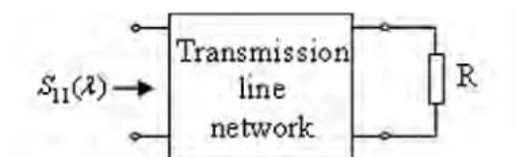
Darlington representation of a transmission line network is given in Fig. 1. Here, S λ11( ) represents the bounded real (BR) input re-flectance function, λ = Σ + Ωj is the conventional Richards vari-able associated with the equal-length transmission lines (Unit ele-ments, UEs), or so-called commensurate transmission lines [8]. In detail, λ=tanh pτ, where p= +σ jω is the complex frequency and
τ
is the commensurate delay of the transmission line. Spe-cifically on the imaginary axis (Σ =0), the transformation takes the form (λ= Ω =j jtanωτ).A compact representation of scattering matrix in terms of three canonic polynomials is represented by Belevitch [6]. For a loss-less two-port, the canonic forms of the scattering matrix is giv-en by [6,7] 11 12 21 22 ( ) ( ) ( ) ( ) ( ) ( ) ( ) 1 , ( ) ( ) ( ) S S S S S h f f h g λ λ λ λ λ λ µ λ λ µ λ λ = − = − − (1)
where µ= −f( ) / ( )λ f λ = ±1. For a lossless two-port with re-sistive termination, energy conversation requires that
( ) ( )T
S λ S − =λ I, (2a)
where I is the identity matrix and “T” designated the transpose of the matrix. The explicit form of (2a) is known as the Feldtkeller equation and given as
( ) ( ) ( ) ( ) ( ) ( ).
g λ g − =λ hλ h− +λ f λ f −λ (2b)
In (1) and (2b), g λ( ) is the strictly Hurwitz polynomial of nth
de-gree with real coefficients, and h λ( ) is a polynomial of nth degree
with real coefficients. The polynomial function f λ( ) includes all transmission zeros of the two-port; its general form is given by
/ 2 2 0
( ) ( )(1 )n
f λ = f λ −λ λ , (3)
where nλ specifies the number of cascaded equal-length trans-mission lines (Unit elements, UEs) contained in the two-port, and
0( )
f λ is an arbitrary real polynomial. According to (3), there may be a finite number of transmission zeros in the right half of the λ −
plane. Realization of transmission line network functions having such factors require, in general, complicated structures like cou-pled lines, Ikeno loops et cetera, which are difficult to implement and, therefore, undesirable [9, 10].
A powerful class of networks contains simple, series or shunt, stubs and equal-length transmission lines only. Series-short stubs and shunt-open stubs produce transmission zeros for λ = ∞, cor-responding to the frequency ω π τ= / 2 and odd multiples there-of. Series-open stubs and shunt-short stubs produce transmission zeros for λ =0 (i.e., ω =0). For such networks, the polynomial function f λ( ) takes the more practical form
/ 2 2
( ) k(1 )n
f λ =λ −λ λ (4)
where nλ is the number of equal-length transmission lines in cas-cade, k is the total number of series-open and shunt-short stubs, and the difference n n−( λ+k) gives the number of series-short
and shunt-open stubs. Here, n denotes the degree of the two-port, which is also the degree of g λ( ). The synthesis of the input im-pedance, Zin( ) (1λ = +S11( )) /(1λ −S11( ))λ , for this case, is accom-plished by extracting poles at 0 and ∞, corresponding to stubs, while equal-length transmission lines are extracted by employ-ing Richards extraction method [1]. Alternatively, the synthesis can be carried out in a more general fashion using the cascade de-composition technique by Fettweis, which is based on the factor-ization of transfer matrices [2]. Also, the algorithm proposed in [5] can be used to synthesize the cascaded commensurate trans-mission lines.
3. Explicit Synthesis Formulae
The three canonic polynomials g λ( ),h λ( ) and f λ( ) are in the following form for cascaded commensurate transmission lines;
1 1 1 0 ( ) n n n n g λ g λ g λ − gλ g − = + K+ + ,
Explicit Synthesis Formulae for
Cascaded Lossless Commensurate Lines
By Metin ŞengülAbstract – In literature, synthesis of cascaded lossless commensurate lines have been realized via some
itera-tive methods. So to be able to obtain the value of an element which is not the first one, the designer has to ob-tain all the values of the elements connected before the desired one. But in this paper, explicit synthesis formu-lae of the networks containing cascaded lossless commensurate lines up to three have been derived analytical-ly, and all the element values can be calculated independently.
Index Terms – Synthesis, Lossless networks, Commensurate lines.
Fig. 1: Darlington representation of a transmission line network.
Brought to you by | Kadir Has University Authenticated Download Date | 11/29/19 7:17 AM
Frequenz 62 (2008) 1-2
17
1 1 1 0 ( ) n n n n hλ hλ h λ− hλ h − = + K + , 2 / 2 ( ) (1 )n f λ = −λ .Firstly, by using the coefficients of these polynomials, the follow-ing dummy parameters and the constant K must be calculated as,
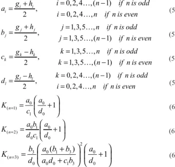
0,2,4 ,( 1) , 0,2,4 , 2 i i i i n if n is odd g h a i n if n is even = − + = = K K (5a) 1,3,5 , , 1,3,5 ,( 1) 2 j j j g h j n if n is odd b j n if n is even + = = = − K K (5b) 1,3,5 , , 1,3,5 ,( 1) 2 k k k k n if n is odd g h c k n if n is even = − = = − K K (5d) 0,2,4 ,( 1) , 0,2,4 , 2 l l l k n if n is odd g h d i n if n is even = − − = = K K (5e) 0 0 ( 1) 1 0 1 n a a K c d = = + (6a) 0 1 0 ( 2) 0 1 0 1 n a b a K d c d = = + (6b) 2 3 0 1 3 0 ( 3) 0 0 0 1 3 0
(
)
1
nb a b b
a
K
d a d
c b
d
=
+
=
+
+
(6c)Then obtain the modified polynomials g and h via the following equations, ( ) ( ) m g λ =g λ ⋅K, (7a) ( ) ( ) m h λ =h λ ⋅K. (7b)
Now calculate the new dummy parameters defined by (5) by using the modified polynomials g λm( ) and h λm( ). Then element values of the network seen in Fig. 2 can be calculated via the equations seen in Table 1.
4. Example
Let us synthesize the network described by the following polyno-mials via the proposed procedure explained in the previous sec-tion and the method given in [5], and then compare the results.
3 2 ( ) 1.3438 0.875 0.625 0.25 h λ = − λ − λ − λ− , 3 2 ( ) 1.6563 3.5 3.125 1 g λ = λ + λ + λ+ , 2 3/ 2 ( ) (1 ) f λ = −λ .
If we calculate the dummy parameters and the constant K, we found the following results,
a0 = 0.375, a2 = 1.3125, b1 = 1.25, b3 = 0.1563, d0 = 0.625, d2 =
2.1875, c1 = 1.8750, c3 = 1.5001, K(n=3) = 0.4
After multiplying the polynomials g λ( ) and h λ( ) by K( 3)n= =0.4, the following new parameters are obtained using the coefficients of the polynomials g λm( ) and h λm( ),
a0 = 0.15, a2 = 0.525, b1 = 0.55, b3 = 0.0625, d0 = 0.25, d2 = 0.875,
c1 = 0.75, c3 = 0.6.
Then via Table 1, the element values are calculated as, 3 0.5, 2 1, 1 0.5, 0.6
Z = Z = Z = R= .
If we solve the same problem via the method in [5], the following results are obtained,
3 0.5, 2 1, 1 0.49999, 0.6
Z = Z = Z = R= .
As can be seen from the above results, explicit formulae give the exact results, but the other method has a very small error. So if the number of commensurate lines is three or less, the proposed syn-thesis procedure can be used precisely.
5. Conclusion
In this work, explicit formulae for the synthesis of cascaded loss-less commensurate lines have been derived analytically. It is shown that if the number of lines is three or less, the derived for-mulae give exact results. Also to be able to find an element value, there is no need to synthesize the network up to this element. Each element value can be calculated independently.
6. References
[1] H.J. Carlin, “Distributed circuit design with transmission line elements“, Proc. IEEE, vol.59, no.7, pp.1059-1081, July 1971.
[2] A. Fettweis, “Cascade synthesis of lossless two ports by transfer matrix factorization“, in R. Boite, Network Theory, Gordon&Breach, 1972. [3] J. Komiak and H.J. Carlin, „Improved accuracy for commensurate line
synthesis“, IEEE Trans MTT, vol: 24, no: 4, pp.212-215, Apr. 1976. [4] M. Hyder Ali and R. Yarlagadda, “A note on the unit element synthesis“,
IEEE Trans Circuit and Systems, vol.cas-25, no.3, pp.172-174, March 1978.
[5] M. Şengül, “Synthesis of cascaded lossless commensurate lines“, IEEE Trans CAS-II, to be published.
[6] V. Belevitch, Classical network theory. San Francisco, CA: Holden Day, 1968.
[7] A. Aksen, “Design of lossless two-ports with mixed lumped and distrib-uted elements for broadband matching“, Ph.D. dissertation, Bochum, Ruhr University, 1994.
[8] P.I. Richards, “Resistor-termination-line circuits“, Proc. IRE, vol.36, pp.217-220, Feb. 1948.
[9] N, Ikeno, “A design theory of distributed constant filters“, J Elec Comm Eng Japan, vol.35, pp.544-549, 1952.
[10] H.J. Carlin and R.A. Friedenson, “Gain bandwidth properties of a distrib-uted parameter load“, IEEE Trans. Circuit Theory, vol.15, pp.455-464, 1968.
Metin Şengül Kadir Has University Engineering Faculty Cibali Campus 34083 Cibali-Fatih, Ýstanbul Turkey Fax: (+90) 212 533 57 53 E-mail: [email protected] Table 1: Explicit synthesis formulae.
Number of Lines 1 2 3 Z1 0 1 1 0 a b c d + + 0 1 1 0 2 0 1 0 2 1 a b c d d d c a a b + + + + 3 1 3 0 2 0 2 1 3 c c d d b a a b b + + + + + + Z2 0 2 1 1 0 2 a a b c d d + + + + 0 00 1 1 33 ( ) a b b a d c b + + Z3 0 2 1 3 1 3 0 2 a a b b c c d d + + + + + + R 0 0 a d 0 0 a d ad00
Fig. 2. Cascaded lossless commensurate line network.
Brought to you by | Kadir Has University Authenticated Download Date | 11/29/19 7:17 AM