Modeling and Simulation Concepts in Engineering
Education: Virtual Tools
Levent SEVG˙I
Do˘gu¸s University, Electronics and Communication Engineering Department, Zeamet Sok. No. 21, Acıbadem / Kadık¨oy, 34722 ˙Istanbul-TURKEY
e-mail: [email protected]
Abstract
This article reviews fundamental concepts of modeling and simulation in computational sciences, such as a model, analytical- and numerical-based modeling, simulation, validation, verification, etc., in relation to the virtual labs widely-offered as parts of engineering education. Virtual tools that can be used in electromagnetic engineering are also introduced.
1.
Introduction
Engineering [1] is the art of applying scientific and mathematical principles, experience, judgment, and common sense to make things that benefit people. It is the process of producing a technical product or system to meet a specific need in a society. Engineering education is a university education through which knowledge of mathematics and natural sciences are gained, followed up by a lifetime self-education where experience is piled up with practice. The four key words mathematics, physics, experience and practice are the “untouchables” of engineering education.
Engineering is based on practice minimums of which should be gained in labs during the university education. However, parallel to the increase in complexity and rapid development of high-technology devices, the cost and comprehensiveness of the lab equipment required to fulfill the aforementioned minimum amount become unaffordable. Computers, other microprocessor-based devices, such as robots, telecom, telemedicine devices, automatic control/command/surveillance systems, etc., make engineering education not only very complex and costly but interdisciplinary as well. The cost of building undergraduate labs in engineering may be a few orders higher than turning a regular PC into a virtual lab with the addition of a card or two. Consequentially, engineering faculties are constantly faced with the dilemma of establishing a balance between virtual and real labs, so as to optimize cost problems, while graduating sophisticated engineers with enough practice. The impact of virtual experimentation and computer simulations is that they are better equipped to understand and use mathematical expressions as well as graphics effectively.
Development of novel computer technologies, interactive multimedia programming languages (e.g., JAVA), and the World Wide Web (WWW) make it possible to simulate almost all of the engineering problems on a computer. With internet access it is now possible to offer students virtual labs via the WWW or CD-ROM as parts of new engineering curricula. The overall effectiveness of modeling and computer simulation in education has been very positive, and this continues to be used and expanded.
On the other hand, technical challenges in engineering today, posed by system complexities, require a range of multi-disciplinary, physics-based, problem-matched analytical and computational skills that are not adequately covered in conventional curricula. Physics-based modeling, observation-based parameterization, computer-based simulations, experimentation via real and virtual labs, model validation and data verification through canonical tests/comparisons are the key issues of current engineering education [2-5].
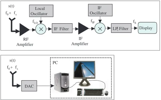
Moreover, technological priorities have been shifting rapidly from analog systems to almost completely digital ones. For example, look at the block diagrams of a conventional and novel radar (or communication) receiver systems in Figures 1a and 1b. The received signal from the receive antenna passes through a series of electronic processes before the information is extracted; first it is amplified and transferred to intermediate frequency (IF) via a microwave mixer, filtered there and then amplified. Then, a second stage mixing followed by a low-pass filtration take place and audio and/or video information is obtained. Almost all of these steps are carried out via electronic amplifiers, mixers and filters, and only audio/video signal may be processed with a computer by using digital-to-analog (DAC) cards. An engineer requires be equipped with strong background in microwave theory and techniques. Figune 1b illustrates a novel radar system which attracts a high attention; the soft radar, where the received signal is digitized just after the antenna system with a high-speed DAC card and the rest is handled on the computer by using various detection, filtration, amplification algorithms. Everything except the antenna in this system is digital and an engineer requires a strong background of signal processing techniques. The essentials of both of these receivers should be covered by the curricula. The problem is how, with what and how much a communication/radar engineer (in specific) is going to be equipped during the four-year engineering education?
The definition of “hands-on” has changed drastically in the last couple of decades. Today, design means endless rounds of modeling and simulation. The design engineers have effectively become computer programmers. Engineers, who build systems whether chips or boards, seem to be doing less and less actual design of circuits, and ever more assembly of prepackaged components. They don’t even layout blocks of circuitry. fLO RF Amplifier Display s(t) f0+ fs Local Oscillator IF Filter fS fIF IF Oscillator LP Filter IF Amplifier DAC PC s(t) f0+ fs
2.
Computational Science: Modeling and Simulation
Computational Science is a novel area of basic and applied research in high-performance computing, applied mathematics, intelligent systems and information technologies. The main purpose is to gather people from universities, industry and governments and enable them work cooperatively for efficient and cost-competitive designs with advanced computing sources, and to enhance science education and scientific awareness. It is a new and cost-effective way of solving problems beyond the reach of most computers, and the outcome is powerful software tools for the students, lecturers, government researchers, and industrial scientists. It is, therefore, timely to discuss modeling and simulation concepts in computational sciences.
Computational sciences require basic understanding of fundamental concepts like modeling, analytical solution, numerical solution, analytical- and numerical-based modeling, simulation, model validation, code verification through canonical tests/ comparisons, accreditation, etc. Analytical solution is the solution based on a mathematical model (usually in differential and/or integral forms) of the physical problem in terms of known, easily computable mathematical functions, such as, sine, cosine, Bessel, Hankel functions, etc. Numerical solution is the solution based on direct discretization of the mathematical representations by using numerical differentiation, integration, etc. Semi analytical-numerical solution is in between these two and is the solution based on partially derived mathematical forms that are computed numerically.
A model is defined as a physical or mathematical abstraction of a real world process, device, or concept. Simulation is concern with modeling of real-world problems. Simulation in engineering usually refers to the process of representing the dynamical behavior of a “real” system in terms of the behavior of an idealized, more manageable model-system implemented through computation via a simulator. Usually, use of modeling and simulation is the most effective, if not the only way to solve complex engineering problems whose analytical solutions cannot be obtained or are yet unavailable. A computer simulator is a program or a series of programs developed to implement and execute simulations with well-defined relations between model objects. These relations are, by definition, mathematical relations, numerical or not.
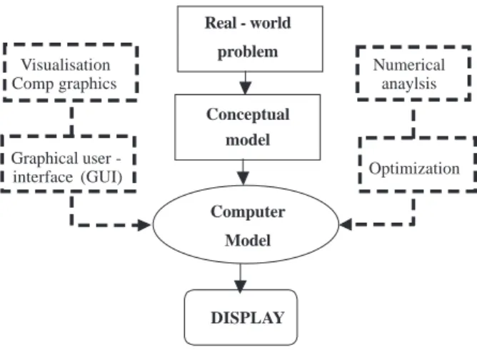
Modeling and simulation is extremely valuable in engineering if based on physics-based modeling and observable-based parameterization. Figure 2 shows a block diagram of a computer model. It starts with the definition of the real-life problem. Its conceptual model is the basic theory behind the real-world problem. Some disciplines have already been in their mature stage in establishing theories. For example, field and circuit theories (Maxwell equations) establish the physics of electrical engineering, well-define the interaction of electromagnetic (EM) waves with matter, and form the basis for a real understanding of electrical problems and their solutions. Modeling and simulation of the “real” problem through the conceptual models in discrete (artificial) environment is called computer model. Visualization and graphical user interface (GUI) design are the computer graphics part of the computer model, while optimization and other tools such as numerical integration and differentiation, interpolation, root search, solving sets of equations, etc., form the numerical analysis part.
Whether analytical or numerical, models need to be coded for numerical calculations on a computer. While the model used in analytical solutions is constructed according to the specific environment, the nu-merical model is general. That is, the problem-specific environment and/or initial conditions are supplied externally to the numerical model together with the other operational parameters. Once they are specified, simulations are run and sets of observable-based output parameters are computed for a given set of input parameters. The computer simulation, based on either analytical-based model or numerical-based model, starts with discretization (it should be noted that discretization changes the problem completely. For exam-ple, relations/differences between mathematically defined Fourier transformation and numerically computed
fast Fourier transformation (FFT) is a good example. Performing FFT in discrete environment introduces periodicity, aliasing, spectral leakage, scalloping loss, etc. which are not inherited in mathematical Fourier transformation [9]). Real - world problem model Conceptual Model Computer Visualisation Comp graphics Optimization DISPLAY Graphical user -interface (GUI) Numerical anaylsis
Figure 2. Basic contents of a computer model; a real-world problem, a conceptual model and the computer model.
The computer model may be accommodated by visualization and optimization tools, a graphical user interface (GUI), numerical analysis tools such as root finding, numerical integration, interpolation algorithms, etc.
The two approaches that can be followed in numerical simulations are closed- and open-form represen-tations. Closed-form solutions are based on an N×N Matrix representation and require matrix inversion algorithms. They are unconditionally stable but require huge matrices as problems size enlarge. Open-form representations are based on a small number of iterative equations, therefore, memory requirements are minimal, but the solution is conditionally stable.
The fundamental building blocks of a simulation comprise the real-world problem being simulated, its conceptual model, and the computer model implementation [10]. The suitability of the conceptual model, verification of the software and data validity must be addressed to make a model credible. Credibility resides on two important checks that must be made in every simulation: validation and verification. Validation is the process of determining that the right model is built, whereas verification is designed to see if the model is built right [10].
3.
Sample Virtual Tools in EE Education
Variety of EM simulation tools have been introduced [7] recently, from radiowave propagation to antenna design, radar cross-section (RCS) calculations to radar simulations, electromagnetic compatibility to bio-electromagnetics, etc. LabView- and Matlab-based virtual instruments (VI) and virtual tools (VT) have also been introduced [8-12]. A few of them are presented in this section (they can be downloaded from http://www3.dogus.edu.tr/lsevgi).
3.1.
An FFT tool
A LabView-based VI DFFT has been prepared to generate and display time/frequency domain behaviors of various signals. The tool may be used to exercise all windowing, aliasing, spectral leakage effects, digital filtration, noise effects, etc. The DFFT is an extremely handy tool for the lecturers who teach FT, as well
as for the students (even for the researchers) who need to do many tests to understand FT problems such as aliasing, spectral leakage, and scalloping loss. The reader may enjoy doing experiments with the DFFT and then may discuss the results. It is really educating to parameterize a time record and write down the expectations first, and then to run the experiment with the presented VT and comment on the results (or vice versa). It is our experience from our environment that without these kinds of numeric tests one can learn but not understand the FT in detail.
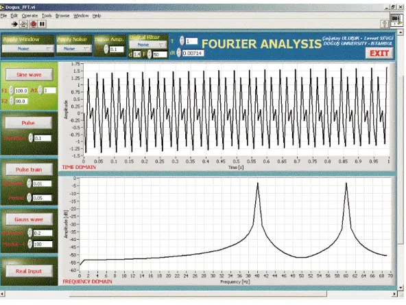
The user may select one of signal types; sinusoids, Gaussian pulse, sine-modulated pulse, pulse train, etc. Noise can be added with a specified signal-to-noise ratio (SNR). A number of window functions may also be applied. Main discretization parameters, the integration period-T, and the sampling interval- ∆ , are supplied by the user from the front panel. The front window of DFFT is given in Figure 3. Here, two equal-amplitude sinusoids with frequencies f1=100 Hz and f2=80 Hz, are shown. The top window presents
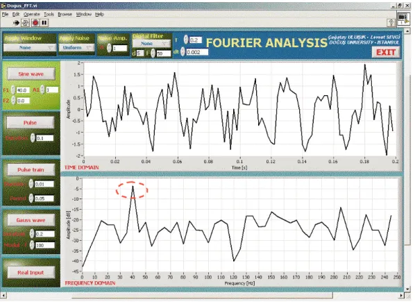
the time plot. The bottom window displays its FFT. The integration time and the sampling interval of this example are T = 1s and ∆ t = 0.00714 s, respectively. These correspond to maximum frequency of 70 Hz, therefore, the two sinusoids fold over 40 Hz and 60 Hz, respectively. Another example is given in Figure 4 which belongs to the illustration of the effects of the added noise. A 40 Hz sinusoid having 1 V -amplitude and added noise with uniform distribution (having zero mean and a variance of 1 V ) is shown. From above equations SNR is found to be 1.5 (or 1.8 dB). It is clearly observed that although the sinusoid is hardly identified in the time domain, the peak at 40 Hz in the frequency domain can still be identified. The theoretical and programming aspects of this VT are given in [8].
Figure 3. The front panel of the DFFT virtual instrument. Two sinusoid problem ( f1 = 100 Hz, f2 = 80 Hz, ∆t = 0.002 s, fmax = 250 Hz, T = 1 s, corresponds to ∆f = 1 Hz).
Figure 4. The front panel to illustrate signal (a sinusoid) plus (uniform) noise effects ( f1 = 40 Hz, A1 = 1, f2 = 0 Hz, T = 0.2 s, ∆t = 0.002 s, uniform noise with 1 V amplitude).
3.2.
A Time Domain Reflectometer tool
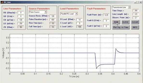
The TDRMeter VT is a multi-purpose package which is design to visualize voltage pulse propagation and reflections from various discontinuities along a TL [9]. It may also be used as a TDR and the user may exercise tests of different type randomly selected terminations and/or faults, and tries to find out what kind of problem exists by analyzing time history of the simulated voltage pulses. The VT can be used both in EM lectures as well as in virtual EM labs. The front panel of TDRMeter is given in Figure 5. Two plots are used for the visualization purposes. The outcome of the FDTD simulations can be given as either signal vs. TL length at each simulation time, or signal vs. time at the specified observation point. The figure on the front panel is reserved for the visualization of pulse propagation/reflections along the TL as the time progresses.
The popup menu at the right top contains a key selection; the TL or the TD Reflectometer. The default selection is the TL where user specifies all input parameters, and with which he/she does simulations to visualize time domain TL effects. The TD Reflectometer selection may be used to locate TL termination and faults. It is designed in a way that the user specifies only the line and source parameters; the load is selected automatically (also randomly), and a fault is introduced at an arbitrary point along the TL so the user can find out its type and/or numerical values (if possible) by only observing/analyzing the output plots, e.g., signal vs. time at the selected point on the TL.
The plot in Figure 5 belongs to a 50 Ω, 0.5 m loss-free homogeneous (uniform) TL excited with a Gaussian pulse source having 10 Ω-internal resistor, and terminated by a resistive load of 100 Ω (the TL is fault-free, i.e., uniform). The simulation time step is 400. Since unit length inductance and capacitor
values are 250 nH/m, and 100 pF/m, respectively, the speed of voltage and current waves along the line is calculated from the limiting case of (6a) to be v = 2 m/s. The TL is divided into 100 nodes therefore ∆x = 0.5/100 = 5 mm. The time step ∆t is calculated to be ∆t = ∆x/v = 25 ps. With this choice the voltage (or current) pulse propagates one node at a time therefore it will take 100 ∆t for the injected pulse to reach the load. The total of 400 ∆t will result in two reflections from the load and two reflections from the source ends. Signal vs. time of a fault-free TL line for the parallel RC termination (RL = 10 Ω,
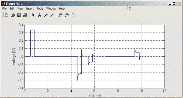
CL = 5 pF) are given in Figure 6. The internal resistor of the source is Rs = 100 Ω. Identification of
each pulse and measurement of the time delays among them certainly yields the TL length, the observation distance from the source or load and the termination type.
Figure 5. The front panel of the TDRMeter package, parallel RC termination, rectangular pulse reflected from the
load (a 50 Ω transmission line, Rs = 100 Ω , pulse width = 400 ps, RL = 10 Ω , CL = 5 pF ), (c) Signal vs. time
on the TL at 0.1 m away from the source.
The TDRMeter can be used to teach, understand, test and visualize the TD TL characteristics; echoes from various discontinuities and terminations. Inversely, the types and locations of fault can be predicted from the recorded data. Any electronic device and/or circuit include TL lines (i.e., coaxial, two-wire cables, parallel plate lines, microstrip lines, etc. therefore have transient EM characteristics.
3.3.
A Filter design tool
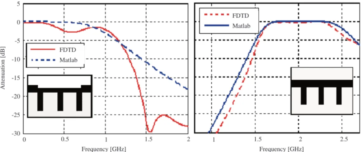
The Matlab-based virtual tool FILTER has been prepared to design LC and microstrip circuit filters [10]. The front panel of the tool is shown in Figure 7. The user may select the filter type from the pop-up menu at top-right, and specifies the frequency characteristic. Filter characteristics and microstripline substrate specifications (dielectric thickness and relative permittivity) are supplied by the user either from the data boxes or by using the sliding bars. The LC filter-prototype and the microstripline equivalent prototype appear at bottom-left. The output is given at right. Here, the order of the filter, values of LC elements, and the dimensions of the microstripline prototype filter are given at this section. The graph at top-right
is for the frequency response of the designed filter. The transfer function vs. frequency (either in linear or in logarithmic scale) is given at this window. Lowpass filter is used as the default type in the front panel. The design examples of a lowpass and a bandpass filters are presented in Figure 8. Here, insertion loss vs. frequency obtained with the VT is compared against another FDTD tool.
Figure 6. Signal vs. time on the TL at 0.1 m away from the source (parallel RC termination, 50 Ω -TL, Rs = 100 Ω ,
pulse width = 400 ps, RL = 10 Ω , CL = 5 pF ).
5 0 -5 -10 -15 -20 -25 -30 Attenuation [dB] FDTD Matlab FDTD Matlab 0 0.5 1 1.5 2 1 1.5 2 2.5 Frequency [GHz] Frequency [GHz]
Figure 8. (a) A third-order lowpass filter, (b) A third order bandpass responses obtained via both FILTER and the
FDTD package.
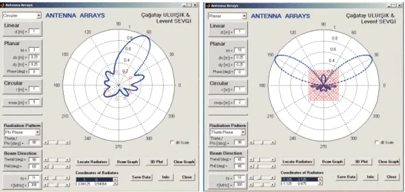
Figure 9. A Matlab VT ANTGUI and radiation pattern of a 10 × 10 planar array of isotropic radiators (i.e., point
3.4.
The antenna array tool
A Matlab-based VT ANTGUI is designed for the analysis of planar antenna arrays of isotropic radiators [11], where the user may locate arbitrary number of radiators to form a linear, a planar or a circular array with beam steering capabilities. It is a nice antenna array analysis package equipped with interesting capabilities. It should be interesting to the user who can design an array by locating a number of radiators arbitrarily just by moving and clicking the mouse, and observe their radiation characteristic in a two-dimensional (2D) polar plot. For example, 10 × 10 planar array and its horizontal radiation pattern at 300 MHz is shown in Figure 9. The user-supplied parameters are listed on the right, some of which may also be changed by using sliding bars. The VT has also a 3D plotting capability as shown in Figure 10 where radiation patterns of different arrays are shown. Two other examples are given in Figure 11.
Figure 10. Typical 3D radiation patterns obtained via the same package.
The VT can be used to design any 2D array and its 2D and 3D radiation characteristics can be investigated. Beam forming capabilities for different locations, number of radiators, as well as for operating frequencies can be visualized. The VT may be used as an educational tool in many undergraduate antenna lectures. It may also be used to validate and verify the FDTD and method of moments (MoM) packages in public domain or, for example the ones supplied in [7]. Moreover, the reader may improve package and add novel features by using the supplied source codes.
3.5.
A ray-tracing propagation tool
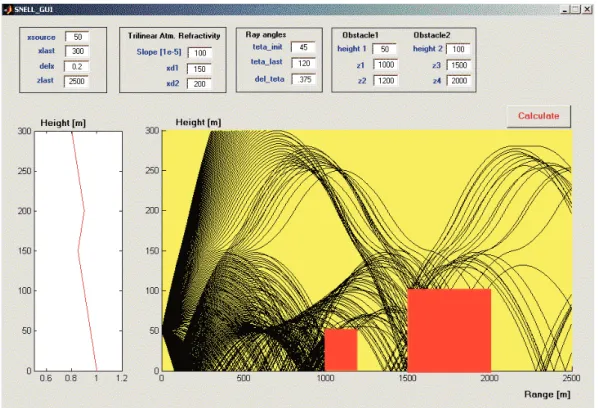
A short and very simple Matlab VT SNELL (a ray-shooting package) is prepared to plot a number of ray paths, with user-specified departure angles, through propagation medium characterized by various linear vertical refractivity profiles and may or may not include one or two obstacles along the propagation path [11]. The only one mathematical relation behind this simulation is the Snell’s law of reflection. Once the parameters are supplied, the 2D propagation medium is divided into slices of horizontal layers of constant refractivity, and Snell’s law is applied consecutively. Figure 12 shows more than hundred ray paths along a propagation medium characterized by a tri-linear vertical refractivity profile with two rectangular perfectly reflecting obstacles. Formation of both a surface duct and an elevated duct between the transmitter and a receiver is clearly observed in the figure.
Figure 12. The SNELL simulator; ray shooting through an atmosphere with a tri-linear refractivity profile and two
non-penetrable rectangular obstacles.
The SNELL VT may be used as an educational tool in various EM lectures, such as, EM Wave theory, Antennas and Propagation, Wireless Propagation, as well as a research tool to predict ducting and/or anti-ducting conditions in the presence of buildings and under various atmospheric refractivity conditions.
3.6.
An SSPE propagation tool
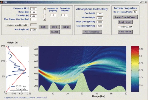
Another, highly effective groundwave simulation VT, the SSPE, based on the well-known FFT-based, longitudinally marching, step by step numerical solution of the 2D parabolic equation which accounts for the one-way (forward) propagation problems, is introduced in [12]. Any kind of a range-dependent non-flat terrain profile can be designed by the user by marking a number of points on the terrain surface by just clicking the mouse. Various refractivity profiles may also be supplied with a few height and slope parameters. The front panel of the SSPE, given in Figure 13, is divided into three sub regions. On top, geometrical and operational parameters are supplied by the user. The command push buttons are also located in this region. The large window at right is the range-height window (where range and height are displayed in kilometers and meters, respectively). In this window, the vertical transmit antenna pattern is supplied at left and propagation is simulated towards right. The user-defined terrain profile is displayed in this window together with the SSPE simulated numerical result which is plotted in 3D as field strength vs. range/height color graphics. Different colors from red to blue correspond to high-to-low level field strength values, respectively. In Figure 13, forward scattering effects of a down-tilted Gaussian beam source is shown.
Figure 13. The SSPE and propagation through bilinear atmosphere over irregular terrain; frequency is 100 MHz,
maximum range 60 km, maximum height 1500, transmitter height 750 m, antenna tilt 2 degrees downwards, and beamwidth is 1 degree.
Another typical scenario showing the formation of an extra surface duct, while establishing a link through an elevated duct occasionally met in a typical ground-to-air communication problem, is given in Figure 14. Here, the propagation through atmosphere with a tri-linear refractivity profile over a rough terrain is shown. The transmitter is tilted 2 degrees upwards and has 1 degree beamwidth antenna at 100 MHz frequency. The characteristics of the elevated ducting conditions are clearly observed in the figure since highly trapping refractivity slope is chosen in this example. The chosen tri-linear refractivity profile may
cause trapping in regions from surface to 400 m, and above 800 m, depending on, for example, transmitter height, antenna tilt, frequency, etc. Because of these double and strong trapping regions, the upward-directed radiated beam splits into two, and propagates partially along the surface and partially through the elevated duct.
Figure 14. Propagation through tri-linear atmosphere over an irregular terrain; frequency 100 MHz, maximum
range 70 km, maximum height 1500 m, transmitter height 250 m, antenna tilt 2 degrees upwards, and beamwidth 1 degrees.
4.
Conclusions and Discussions
Virtual labs have become attractive tools in engineering education. The overall effectiveness of modeling and simulation (i.e., virtual experimentation) in engineering education is very positive, and this continues to be used and expanded. The impact on students is that they are better equipped to understand and use mathematical expressions (as long as they understand basic concepts discussed above). Some comments on novel engineering education curricula may be listed as:
• Novel education techniques such as problem-based learning, inquiry-based teaching should be discussed in detail under available teaching resources (i.e., personnel, labs, classroom capacities, number of students, etc.) and smooth adaptation should be made accordingly.
• Subjects like energy sources and conversion, environment, electromagnetic radiation, light and sound, thermodynamics, material science should be included in engineering curricula.
• Engineers should be well equipped to deal with data acquisition, correlation, models, epidemiology, risk management, information-based decision making, uncertainty and bounds of science.
• Basic lectures, such as measurement techniques should be improved accordingly and concepts like accuracy, precision, resolution should be well taught. Error analysis is also another important concept that should be well taught.
• Hands-on practice and training is a must in engineering education. Although, labs and test instruments have been simulated as virtual reality environments, which may be as good as the real environment, students still need hands-on training.
• Computer simulations are as necessary as hands-on training; therefore, modeling and simulation lectures should be included in engineering programs.
• Engineers become more publicized in parallel to technological developments. Therefore, lectures like Science Technology and Society, or Public Understanding of Science should be included in the engineering curricula.
References
[1] American Society for Engineering Education web site (http://www.asee.org).
[2] L.B. Felsen (ed.), “Engineering Education in the 21st Century: Issues and Perspectives,” IEEE Antennas and
Propagation Magazine, 43 (6), pp. 111-121, 2001.
[3] L.B. Felsen, L. Sevgi, ”Electromagnetic Engineering in the 21stCentury: Challenges and Perspectives,” Special
issue of ELEKTRIK, Turkish J. of Electrical Engineering and Computer Sciences, Vol.10, No.2, pp.131-145, 2002.
[4] L. Sevgi, ”Challenging EM Problems and Numerical Simulation Approaches,” A Special Workshop/mini Sym-posium on Electromagnetics in Complex World: Challenges and Perspectives, University of Sannio, Benevento, Italy, Feb. 20-21, 2003.
[5] L. Sevgi, ”EMC and BEM Engineering Education: Physics based Modeling, Hands-on Training and Challenges”, IEEE Antennas and Propagation Magazine, Vol. 45, No.2, pp.114-119, 2003.
[6] L. Sevgi, ˙I.C. G¨oknar, “An Intelligent Balance on Engineering Education, IEEE Potentials, Vol. 23, No 4, pp.40-43, Oct/Nov. 2004.
[7] L. Sevgi, Complex Electromagnetic Problems and Numerical Simulation Approaches, IEEE Press – John Wiley and Sons, NY 2003.
[8] L. Sevgi, C¸ . Uluı¸sık, ”A LabView-based Virtual Instrument for Engineering Education: A Numerical Fourier Transform Tool”, ELEKTRIK, Turkish J. of Electrical Engineering and Computer Science, this issue, 2005.
[9] L. Sevgi, C¸ . Uluı¸sık, ”A Matlab-based Transmission Line Virtual Tool: Finite-Difference time-Domain Reflec-tometer”, IEEE Antennas and Propagation Magazine, Vol. 47, No. 6, Dec. 2005.
[10] G. C¸ akır, S. G¨und¨uz, L. Sevgi, ”Broadband Filter Design using the Analogy Between Wave and circuit theories”, CCN Complex Computing Networks, Springer Proceedings in Physics, Vol. 104, pp. 141-148, Feb. 2006.
[11] L. Sevgi, “A Ray Shooting Visualization Matlab Package for 2D Groundwave Propagation Simulations”, IEEE Antennas and Propagation Magazine, Vol. 46, No 4, pp.140-145, Aug 2004.
[12] L. Sevgi, C¸ . Uluı¸sık, F. Akleman, ”A Matlab-based Two-dimensional Parabolic Equation Radiowave Propagation Package”, IEEE Antennas and Propagation Magazine, Vol. 47, No. 4, pp. 184-195, Aug. 2005.
[13] L. B. Felsen, F. Akleman, L. Sevgi, ”Wave Propagation Inside a Two-dimensional Perfectly Conducting Parallel Plate Waveguide: Hybrid Ray-Mode Techniques and Their Visualisations”, IEEE Antennas and Propagation Magazine, Vol. 46, No.6, pp.69-89, Dec 2004.
[14] L. Sevgi, C¸ . Uluı¸sık, ”A Matlab-based Visualization Package for Planar Arrays of Isotropic Radiators”, IEEE Antennas and Propagation Magazine, Vol. 47, No. 1, pp. 156-163, Feb 2005.