Input sequence estimation and blind channel identification in HF communication

(1)

INPUT SEQUENCE ESTIMATION AND BLIND CHANNEL IDENTIFICATION

IN HF COMMUNICATION

M . Khames B. H. Miled and Orhan Arzkan

Department of Electrical and Electronics Engineering,

Bilkent University, Ankara, TR-06533 TURKEY.

Phone & Fax: 90-312-2664307,

e-mail: khames@ee.bilkent .edu. t r and oarikaneee. bilkent .edu. t r

ABSTRACT

A new algorithm is proposed for reliable communication over H F tropospheric links in the presence of rapid channel variations. In the proposed approach, using fractionally spaced channel outputs, sequential estimation of channel characteristics and input sequence is performed by utilizing subspace tracking and Kalman filtering. Simulation based comparisons with the existing algorithms show that the proposed approaches significantly improve the performance of the communication system and enable us t o utilize HF communication in bad conditions.

1. INTRODUCTION

Digital communication systems usually suffer from inter- symbol interference, ISI. This phenomenon is known to be caused by the channel memory, which spreads the transmitted symbols in time, or due to time-varying multi-paths. To combat the limitation in performance due to such factor, blind channel equalizers are usually built within receivers. In the case of H F communication links, channel equalization becomes a difficult task due to the additive noise and the channel time-variation which leads t o a degradation in the performance of the equalizer as time progresses. Typically, a periodic transmission of a training sequence is utilized, reducing the channel bandwidth. Moreover, even with the use of such periodic sequences, the equalizer may fail and result in a down-link in poor conditions.

Recent research in the subject, tried to come up with robust equalizers [l], [2], [3], and to avoid training sequences [4]. A commonly used technique is fractional sampling [ 5 ]

which introduces channel diversity and reduces the noise variance [6]. In this paper, based on a slowly time-varying channel assumption, an iterative algorithm is proposed for the joint estimation of the input sequence and channel characteristics. Simulation based comparisons with the existing algorithms show that the proposed approaches significantly improve the performance of the communication system and enable us to utilize H F communication in bad conditions even at 10 dB SNR.

2. INPUT SEQUENCE ESTIMATION AND

CHANNEL IDENTIFICATION

In H F communication, transmitted signals may be received through multiple paths in the atmosphere as they are re- flected by distinct ionospheric layers.

A practical model for

the H F channel is shown in Fig. 1, where an improved ver- sion of the Watterson model [7] with diffuse layers is used. Specifically, the channel transfer function is described as

a sum of shifted Gaussian functions, each of which corre- sponds t o a distinct transmission path. The corresponding baseband channel model is:

y(t) =

Gi(t)[z(t)

*

f i ( t - si)] (1)

a

where

f i ( t )

= k e x p ( $ ) ,

Gi(t)

is the amplitude dis- tortion term.

Assuming oversampling with a factor of M, equivalent baseband model t o the communication system is the single- input multiple-output, SIMO, system shown in Fig. 2. In

the following, the input symbols z[n] are assumed to be of binary. The sequences vi[n] and yi[n] represent, respectively, the additive noise and the output of the sub-channels. In H F communication, as in most of the communication systems, the ultimate purpose is to be able to estimate the transmitted symbol sequence as reliable as possible at the receiver. However, since the medium of transmission is the H F tropospheric channel, the receiver has to provide estimates to the input symbols in the absence of a precise channel transfer function. Another important problem in the H F communication is the identification and tracking of the time-varying HF channel response when the channel input sequence is unknown. In the following approach, the problems of blind channel identification and input symbol estimation are iteratively solved by making use of the solution to one t o get a solution to the other.

2.1. Input Sequence Estimation

Assuming that the individual channels are of finite order L, their outputs can be written as:

yi[n] = hrnxn

+

~i[n], i = 1,. .

.

,

M ( 2 )

(2)

wherex, = [z[n],z[n-l],

...,

~ [ n - L + l ] ] ~ is thevector of channel inputs. The input sequence estimation problem can be stated as:

given y,[n] = h:,x,

+

vi[n], for 1 i

5

M , estimate 4 7 2 1 E

{ F A } ,

for n

2

0.

The above formulation is nonlinear in the unknowns x, and hi,, which are in a multiplicative form. A straight forward approach would be the use of extended Kalman filter [8], but it has a high computational cost and does not take advantage of the binary nature of the input sequence. To overcome the nonlinearity problem, we provide an alternative approach where the existence of an initial estimate to the channel response is assumed. Such an estimate can be obtained by using a short training period. Then recursively, the input sequence will be estimated by using the estimated channel and the channel estimate will be updated by u$ng the estimated input sequence. Once reliable estimates hi,, are given, the input sequence estimation can be recast in the following simplified form:

given yiin] =

ii:,x,

+

vi[n], for 1

5

i

₅

M , estimate

4.1

E

{ F A } ,

for n 2 0 .

Different approaches such as the Kalman filter [8] and the Viterbi algorithm can be suggested as solutions to the above formulation. In this paper we propose a sub-optimal but very efficient estimator for the input sequence.

Given the past input symbols z [ n

-

K],

.

,

z [ n - L

+

11, we define x9,, q = 1,. .

. ,

2 K as the possible vector values of x, with the last K input symbols are fixed, i.e,

x

:

=

[ A . .

. A

z[n - K ] . . . x [ n

-

L

+

111’. Define the error terms as:

= Y i [ n - IC] - h T , - i ~ E - k . (3)

Then estimate the input sequence as:

where cr: is the variance of vi[n] which is assumed to be known.

In [6], it’s shown that this approach can be implemented with a computational cost of ( L

+

K ) M in contrast t o

M L 2

+

K M

multiplications fequired by a straight forward optimizer. Note that in (3), hi,,-1 was used as an estimate of all hi,,-k, k = 1,. .

. ,

K . Such an approximation is al-

lowed as far as the variation in the channel response is slow enough.

2.2. Channel identification

The identification problem can be stated as follows :

given yi[n] = xzhi,,

+

v.[n], for 1

<

i

5

M , estimate hi,, for n 2 0 and

15

i < M .

The above formulation is nonlinear in the unknowns x, and hi,, which are in a multiplicative form. Assuming that

reliable estimates of the input sequence is obtained as a result of 4, the channel identification can be performed as :

given y;[n] = %:hi,, +v;[n], for

15

i

5

M , estimate hi,, for n 1 0 and 1

si

5 M .

In the following, it is assumed that the channel characteristics remain stationary within the short duration of the channel response which is typically in the order of 10 input symbol durations. This stationarity is modeled as a slowly time-varying low-ranked subspace which contains the most recent channel response vectors in it. By tracking the variation of this channel response subspace, more reliable identification of the channel is made possible. In the proposed approach, by using the available estimates to the input sequence z [ n ] , an adaptive filter is used t o get an estimate h, of the oversampled channel response vector h,. Then, a subspace tracker makes use of this estimate t o update the subspace basis. Finally a more refined estimate h, is obtained by a projection onto the updated subspace. Estimates h, are obtained by using the following state- space representation :

h, = h,-1

+

b,,

Y n = Ghn

+

v n ,

( 5 ) (6)

where b, is the innovation in h,, C, = [ c , , ~ , . . .

,

c , , M - I ] ~ and c , , ~ = [z[n]OTz[n - 11 . . . z[n

-

L

+

1]OTIT. The zero vectors in c , , ~ are of length M - 1 and the vectors c,,i, i = 1,. . .

,

M are obtained by shifting the vector c , , ~ i times t o the right in a circular manner.

By using the Kalman filter [ 8 ] , the required estimate

h,

can be obtained in O ( ( M L ) 3 ) number of multiplications. Fortunately, a reasonable trade-off between the performance and computational load can be made by tracking

only one sub-channel, i.e., h y , , , and approximate the oth- ers with linear interpolations of the former. In this case, the state-space equations become :

h ~= h ~ , ~ - l , ~

+

d n ,

Yn = Cnhg,,

+

v n

+

v n .

( 7 ) ( 8 )

-

where

d,

represents the innovation in h a , , and q,, is a noise vector compensating the approximation error intro- duced by linear interpolation. The measurement matrix C, = [ATx, , .

.

A L x , ] ~ , where the matrices Ai’s refer to

the appropriate linear interpolation operators.

A

further simplification in the output equation (8) can be obtained by assuming all Ai’s as the identity operators :

2

-

A

Yn = Cnhy,n

+

v n

+

v n , (9)

-

where C , = [x, .

.

. x , ] ~ . As shown in [6], this simplification reduces the complexity of the Kalman filter t o O ( L 2 ) .

In all the previously described models, the innovation in the state vectors is modeled as an additive white noise. This implies that its covariance matrix is:

Qd = ~ V ~ I L

,

(10)

(3)

where 0,” is the noise variance. In [6], a more realistic form

for Qd is proposed, which reflects the correlation between the innovation and the estimated state vector :

l h ~ , ” ~ l ~ - ~ l l ~ + ~ l ~ h l ~ ~ ~ ~ ~ l l ~ + l ~ ~ , ~ ~ ~ ~ + ~ l l ~

where kJ = 4

The Kalman filter, although optimal in the MMSE sense, provides noisy estimates of the channel transfer function. To remove such a noise, we make use of subspace tracking methods. In other words, under the smooth time-variation assumption, the matrix H = [hn-.w

. .

.

h,] is of low rank. Its column space is the same as the one of HHT which is the channel covariance matrix over a time interval of length N + 1 . Hence by tracking the eigenspace of the channel covariance matrix, based on the estimates given by the Kalman filter, we can remove most of the noise components. In the literature, various algorithms that can accomplish such a task were proposed. In our approach, we chose the algorithm LORAF 1 presented in [9], which is a low rank

adaptive filter. This algorithm tracks the? dominant eigenvalues of the covariance matrix Qi = E { h , h:}, and their corresponding eigenvectors. With an appropriate choice of

T , the effective dimension of the subspace, the noise can be significantly removed from the signal.

Once the eigenvalues and eigenvectors are obtained, the channel impulse response can be re-updated by projecting h, on to the subspace of eigenvectors :

The three different state-space descriptions together with the two different formulations of Q d (or Qb) suggest six different algor.it;lims that were explicitly stated and compared through different simulations in [6]. In this paper, we present the algorithm KFST, shown in Table 1, which is the best choice based on its performance and computational cost.

3. SIMULATION RESULTS

In this section, simulation based comparison results of the proposed KFST algorithm and two other alternative approaches are presented. The reference algorithms are de- noted as “FTF” and “Sl” (System l ) , which were proposed in [l] and [2], respectively. The former is an efficient fast transversal filter. The second describes the channel as linear combination of a subspace basis and keeps track of the subspace vectors and the corresponding coefficients through recursive projections. However, the orthogonality property of the basis vectors might be lost as time progresses which requires periodic training intervals during which the Gram- Schmidt process is applied.

Table 1: Channel identification algorithm, KFST

In the simulations, we make use of 1000 bits of binary

data with symbol spacing T and sampling period

$.

The channel transfer function is simulated as given in 1 by using three shifted Gaussian functions, corresponding to three distinct tropospheric paths with total duration of 10 T. The oversampling factor is chosen as M = 8. We con- sider slow and rapid variations, SV and RV respectively. In both cases, it is assumed that the channel characteristics remain stationary within the short duration of the channel response which is typically in the order of 10 input sym- bol durations. The signal t o noise ratio is chosen as 23 dB and 10 dB and represented as H, high, and L, low, respectively. In each case, the algorithms are tested over ten different noise realizations. The error measure is defined as steady state.

4721 = 20 log lhn-h711alle lh,l,,, and cave is the mean of ~ [ n ] in the

To examine the channel identification performance of the different algorithms, the latters were simulated in the open-eye case. The corresponding results are shown in Ta- ble 2. The fast transversal filter shows high channel error in the case of low signal-to-noise ratio. The algorithm S1 is simulated with two different values of its parameter b. For

b = 0.0095, the average channel estimation error is slightly higher than the one given by KFST. As seen in this table, KFST has a robust performance under the different conditions.

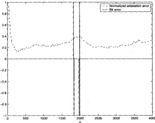
In the case of unknown input sequence, we couldn’t make any of the reference algorithms converge, even for slow time-variation and high signal-to-noise ratio. In fact, they show large burst errors and poor estimation of the channel response. however, as seen in Fig. 3, the proposed KFST algorithm establishes convergence with low bit error rates and robustly recovers from the committed bit errors.

(4)

I

SV/H SV/L RV/H F T F -20.747 -7.534 -17.978 Sl(0.095) -17.412 -4.841 -4.956 Sl(0.0095) -25.578 -20.140 -17.352

KFST -24.086 -20.207 -21.374

Table 2: Average logarithmic error (in dB), in the open-eye case: known input sequence.

RV/L -7.351 -4.956 -16.468 -17.214 c a v e BER

Table 3: Average logarithmic error (in dB), and bit-error

rate in the blind case for KFST.

-15.506 -12.638 -16.533 -11.148

0 0 0 0.022

4. CONCLUSIONS

I I n

’0 5CU 1000 1500 2000 2500 3ooo 3500

The problems of input sequence estimation and blind channel identification in HF communication are investigated. A sub-optimal delayed input sequence estimator is developed and a new channel identification algorithm, KFST, is proposed. The latter is a two-step estimator, making use of a cascade of a Kalman filter and a subspace tracker. Simu- lation results showed reliable channel identification in the open-eye case. In the blind case, the input sequence estimator, operating together with KFST algorithm, had a robust behavior in recovering from input decision errors. When compared to alternative approaches, the proposed algorithm was superior. Even in bad tropospheric conditions when the channel is rapidly varying, the input sequence is estimated reliably.

4030

LL]

Figure 1:

A

multi-path channel model with diffused ionospheric layers.

5. REFERENCES

(11 S. Hariharan and A. P. Clark, “HF channel estimation using a fast transversal filtering algorithm,” I E E E Trans. Acoust., Speech, and Signal Process., vol. 38,

no. 8, pp. 1353-1362, 1990.

(21

A.

P. Clark and A. Hariharn, “Efficient estimators for an HF radio link,” IEEE Trans. o n Communications, vol. 38, no. 8, pp. 1173-1180, 1990.

[3] B. Farhang-Boroujeny, “Channel equalization via channel identification: Algorithms and simulation results for

W YM In1 Figure 2: Multi-channel filter model of the baseband equiv-

alent of the communication system.

Figure 3: Simulation result of blind input symbol estima-

tion and channel identification experiment carried a t low

SNR

and rapidly changing channel conditions. The dashed curve is the normalized channel estimation error and the continuous curve is the symbol estimation error.

rapidly fading hf channels,” I E E E Trans. o n Commu- nications, vol. 44, no. 11, pp. 1409-1412, 1996.

[4] J. Labat,

0.

Macchi, and C. Laot, “Adaptive decision feedback equalization: can you skip the training period,” I E E E Trans. o n Communications, vol. 46, no. 7, [5] L. Tong and

S.

Perreau, “Multichannel blind identification: from subspace to maximum likelihood methods,” Proc. I E E E , vol. 86, no. 10, pp. 1951-1968, 1998. [6]

M.

K. B. H. Miled, “Input sequence estimation and

blind channel identification in hf communication,” Mas- ter’s thesis, Bilkent University, 1999.

[7] C. C. Watterson, G. G. Ax, L.

J .

Demmer, and C.

H.

Johnson, “An ionospheric channel simulator.” unpub- lished ESSA Tech. Memo ERLTM-ITS 198, pp. 1-44, 1969.

[8] C. K. Chui and G. Chen, Kalman Filtering with real- time applications. Berlin Heidelberg: Springer-Verlag, second ed., 1991.

[9] P. Strobach, “Low-rank adaptive filters,’’ I E E E Trans. Signal Process., vol. 44, no. 12, pp. 2932-2947, 1996.

pp. 921-930, 1998.