Resonant and coherent transport through Aharonov-Bohm interferometers with
coupled quantum dots
V. Moldoveanu,1,2 M.Ţolea,1 A. Aldea,1and B. Tanatar3
1National Institute of Materials Physics, P. O. Box MG-7, Bucharest-Magurele, Romania 2Centre de Physique Théorique-CNRS, Case 907 Luminy, 13288 Marseille Cedex 9, France
3Department of Physics, Bilkent University, Bilkent, 06800 Ankara, Turkey
共Received 21 May 2004; revised manuscript received 13 October 2004; published 31 March 2005兲 A detailed description of the tunneling processes within Aharonov-Bohm 共AB兲 rings containing two-dimensional quantum dots is presented. We show that the electronic propagation through the interferometer is controlled by the spectral properties of the embedded dots and by their coupling with the ring. The transmit-tance of the interferometer is computed by the Landauer-Büttiker formula. Numerical results are presented for an AB interferometer containing two coupled dots. The charging diagrams for a double-dot interferometer and the Aharonov-Bohm oscillations are obtained, in agreement with the recent experimental results of Holleitner
et al.关Phys. Rev. Lett. 87, 256802 共2001兲兴 We identify conditions in which the system shows Fano line shapes.
The direction of the asymetric tail depends on the capacitive coupling and on the magnetic field. We discuss our results in connection with the experiments of Kobayashi et al.关Phys. Rev. Lett. 88, 256806 共2002兲兴 in the case of a single dot.
DOI: 10.1103/PhysRevB.71.125338 PACS number共s兲: 73.23.Hk, 85.35.Ds, 85.35.Be, 73.21.La
I. INTRODUCTION
The electronic transport through Aharonov-Bohm rings with embedded quantum dots 共QD’s兲 is a new subject in mesoscopic physics whose complexity competes with the al-ready “classical” problem of persistent currents in closed loops.
Inserting one dot in a ring Yacoby et al.1 studied for the first time the transport properties of such systems. The ob-served Aharonov-Bohm共AB兲 oscillations of the source-drain signal as the magnetic field is varied proved that the tunnel-ing current through the dot is partially coherent. The experi-ment presented a striking behavior of the transmittance phase as a function of the gate voltage applied on the dot, at each transmittance peak the phase jumps by . Due to the two-lead geometry used in this experiment the conductance obeys the Onsager relations and as shown in Ref. 2, this imposes a rigidity of the transmittance phase共0 or兲. Later on Shuster
et al.3,4employed a many lead geometry, the phase evolution being obtained as well as the expected Aharonov-Bohm os-cillations. The experimental geometry was generalized by Holleitner et al.5 who measured the current through a double-dot AB interferometer 共one QD in each arm of the ring兲. The main achievement of their setup is that the dots can be coherently coupled and hence the transport becomes more complex. They have also found AB oscillations of the current and emphasized the formation of coherent molecular states in the two dots. Finally, a recent experiment6 with a two-dot AB ring was performed in a four-lead geometry, the measured transmittance showing peaks in several regimes of the capacitive coupling of the ring. Notably, the phase of the transmittance presents the same increment withwhen one dot is set to resonance and the capacitive coupling of the second dot is varied around a peak.
A closely related problem is the Fano feature of AB inter-ferometers. As reported in Ref. 7 a one dot AB
interferom-eter shows asymmetric line shapes for the transmittance as a function of the plunger gate voltage, the typical proof of the Fano effect,8–10 namely the interference between states be-longing to continuous and discrete spectra.
The transport properties of AB interferometers containing QD’s were theoretically studied by two techniques, the scat-tering approach and the Keldysh formalism in the tight bind-ing picture. The scatterbind-ing theory was successfully used in Refs. 11–13 to describe the physics of one-dot interferom-eters, including specific properties of the transmittance phase. The S matrix of the scattering problem is computed by writing the Born expansion for the T-operator, the conduc-tance being thereafter obtained via the Landauer-Büttiker formula.
In the tunneling picture the net current from one lead to another is computed by perturbation theory and nonequilib-rium Green function techniques. Within this approach one can discuss in detail the co-tunneling spin-dependent pro-cesses and finite bias transport.14 As discussed recently by Kubala and König15both approaches are equivalent, in spite of the differences between the Hamiltonians共in the tunneling picture the coupling between the ring and dots does not ap-pear explicitly兲.
The way in which the experiments with AB interferom-eters can indeed provide the transmittance phase is a subtle point that involves the explicit geometry of the leads used to break the unitarity of the two-lead system.16–19
In the present work we study systematically the tunneling and coherence properties of AB interferometers with QD’s, particular attention being payed to the geometry used in the experiments of Holleitner et al.5The idea behind the calcu-lations presented below is the following. The transmittance of the interferometer as a whole is first related to its Green function, by the Landauer-Büttiker formula. Second, it is shown that this Green function can be expressed in terms of two Green functions that describe separately the ring and the
dots system in the presence of the leads. The ring, lead-dots, and ring-dot couplings appear as non-Hermitian self-energies of an effective Hamiltonian. The latter is obtained by the Feschbach formula20,21 which is a useful tool when dealing with Hamiltonians of coupled subsystems. We point out that this step is necessary in order to obtain detailed information about the complex processes within the interfer-ometer. The resonant transport through the device is dis-cussed in connection with the spectral properties of the dots system embedded in the interferometer. Our approach shows clearly that the important role in the resonant transport pro-cesses is played by the dots inserted in the ring, the latter providing in turn the suitable geometry for quantum
coher-ence.
We do not consider in this paper the Coulomb repulsion because interaction effects on the transport properties of single and coupled dots were studied extensively in the pre-vious papers22–24and all the analysis presented there remains valid here. The Coulomb interaction can be however easily included in our formalism in the Hartree approximation and the charging effects are satisfactorily described by this ap-proach共see Ref. 11 for a similar discussion of the interaction effects in a one-particle approximation兲. The main topics we consider in this work are the tunneling and coherence prop-erties of AB interferometers. The Kondo-type effects which are a subject in itself are not discussed here.
The formalism is presented in Sec. II. Numerical results are discussed in Sec. III in connection with the experimental findings, a qualitative agreement being found. Since we have considered two-dimensional quantum dots the magnetic field dependence of the eigenvalues of the coupled dots system is no longer negligible as in the case of a dot modeled by a single site. It will turn out that the drift of the levels in magnetic field affects the interferometer transport properties. Moreover, the interferometer regime of the device 共namely the one that exhibits AB oscillations兲 is more difficult to reveal. Section IV summarizes the main results and ends the paper.
II. FORMALISM
This section contains the theoretical framework we use to study the electronic transport in Aharonov-Bohm interferom-eters with coupled quantum dots. The Hamiltonians are writ-ten in the tight-binding共TB兲 representation which is particu-larly useful both for describing complex geometries and performing numerical computations. We consider a general interferometer that consists of an arbitrary number of two-dimensional共coupled兲 quantum dots embedded in a 1D me-soscopic ring having N sites. Some of these sites are shared with the dots, which are coupled to each other by tunneling Hamiltonians simulating the tunable barriers patterned in ex-periment. The quantum dots are described as finite two-dimensional共2D兲 plaquettes.
The electrons reach and leave the interferometer through ideal one-channel semi-infinite leads attached on the ring or directly on the dots. The Hamiltonian of the whole system has the form
H = HI+ HL+ HtunLI, 共1兲 with
HI= HD+ HR+ Htun
RD
. 共2兲
HI is the Hamiltonian of the interferometer, HLand HR de-scribe the leads and the truncated ring, i.e., what is left from it after removing the dots共the notations can be identified as well from Fig. 1 which represents a double-dot interferom-eter兲. The magnetic flux through the ring appears in HRin the
Peierls representation as magnetic phases attached to the hopping constants along the truncated ring. Their explicit form is obtained by using for example the Landau gauge.
HtunLI and HtunRD are the lead-interferometer and ring-dots tun-neling Hamiltonians, Htun LI = HLI+ HIL=L
兺
␣ 共兩0␣典具␣兩 + 兩␣典具0␣兩兲, 共3兲 HtunRD= HDR+ HRD=兺
m 共e−im兩m典具0m兩 + eim兩0m典具m兩兲. 共4兲 Here L, are the corresponding hopping parameters and0␣共0m兲 are the nearest sites to the contact points␣共m兲 be-tween lead-interferometer and ring-dots.
m is the Peierls phase associated with the pair of sites
兩0m典, 兩m典. Finally HDis the Hamiltonian of the coupled dots
which is also written in the Peierls representation. It includes the individual Hamiltonian of each dot HDk,
HDk= − eV k
兺
i苸QDk 兩i典具i兩 + tD兺
具i,i⬘典 e2iii⬘兩i典具i⬘
兩 共5兲and the interdot tunneling term Htun共int兲, depending on the coupling constantintwhich is the same for each pair of dots 兵k,k+1其. We point out that the dots embedded in different arms of the ring can be coupled as well, allowing thus com-plicated electronic trajectories within the system. The con-stant term Vkfrom the diagonal part of each HDkmimics the
FIG. 1. Schematic picture of a two-dots Aharonov-Bohm inter-ferometer. The thick solid line represents the truncated ring共R兲. The dashed contour surrounds the interferometer共I兲.␣,  are the sites where the leads are connected to the interferometer and a , a⬘, b , b⬘ are the contact points between ring and dots.
plunger gate voltages used in experiments to tune the dots to resonance, 具i,i
⬘
典 denotes the nearest neighbor summation and tDis the hopping integral on dots.The conductance matrix g␣ of a mesoscopic system at zero temperature coupled to leads is given by the Landauer-Büttiker formula共see Ref. 25 for a rigorous derivation兲
g␣共EF兲 =e 2 hT␣共EF兲 = 4 e2 h L 4 tL2sin 2k兩具␣兩G eff共EF+ i0兲兩典兩 2, 共6兲 ␣⫽,
where T␣共EF兲 is the transmittance, 兩␣典, 兩典 are sites located
on the ring or dots that are coupled to the leads,
EF= 2tLcos k is the Fermi energy of the leads and tL is the
hopping integral on leads. The main quantity in Eq.共6兲 is the effective resolvent of the system in the presence of the leads 共see Ref. 22 for more details兲. In our case Geff共z兲=关Heff共z兲 − z兴−1, where the effective Hamiltonian is defined as
Heff共z兲ª HI−L 2 1共z兲
冉
兺
␣r 兩␣r典具␣r兩 +兺
␣d 兩␣d典具␣d兩冊
共7兲and acts in the Hilbert space of the interferometer HI only and embodies the influence of the leads at the contact points with the ring which we denote兵␣r其 or the dots 兵␣d其 through
the non-Hermitian terms above 共these terms represent the so-called leads’ self-energy, see Ref. 26兲. The notation 1共z兲=共z⫿
冑
z2− 4tL2兲/2 关⫿ shows that z belongs to the upper 共lower兲 half-plane兴 and we choose Re z⬍2tL. In the sequel
we take for simplicity e = h = tL= 1.
In the previous papers22,24 we used simpler effective Hamiltonians. In the particular case of a single dot weakly coupled to leads共see Ref. 22兲 Eq. 共6兲 gives at once the trans-mittance peaks共as a function of the plunger gate voltage V兲 which are related to spectral properties of the dot. Actually the effective Hamiltonian of the dot has resonances with small imaginary part located near the eigenvalues of the iso-lated dot. Similarly, if Heff共z兲 describes an array of identical dots one can obtain and explain the splitting of the Coulomb peaks as a function of the interdot couplingint in terms of the nearly identical spectra of the dots. Moreover, if the in-terdot Coulomb interaction is neglected, the effective Green function can be expressed only in terms of one dot Green function by a recursive formula.
Here formula共6兲 is not of much use because even if the transmittance peaks can be obtained from it by inverting nu-merically the finite matrix of the effective resolvent, one can-not distinguish between the different paths that an electron can follow. Indeed, due to the ring geometry and to the cou-pling between the dots the transport within the device is very complex. Besides that, in the experiments the metalic gates defining the dots are patterned in the ring arms while the incident electrons from leads enter the ring freely. This means that L⬃1, thus a discussion in terms of the
reso-nances of HI is useless. These drawbacks are only apparent and one can rewrite Geff in a suitable way to recover the missing details. The first step is to decompose the Hilbert space of the interferometer asHI=HD丣HRwhereHD共HR兲
is the Hilbert space of dots 共ring兲. We denote then by
P , Q the projectors on these spaces. P , Q are nothing
else but families of on-site projections 兩i典具i兩 from the coupled dots system and the ring. Next, observe that HtunRDis a small off-diagonal perturbation with respect to
HD−L21共z兲兺␣d兩␣d典具␣d兩 and HR−L
2
1共z兲兺␣r兩␣r典具␣r兩 viewed
as non-Hermitian operators inHDandHR. This allows us to use the Feschbach formula20,21which expresses the effective resolvent in the following form关see Eq. 共6.1兲 from Sec. VI B in Ref. 21兴:
Geff共z兲 = GeffR 共z兲 + 关1 − GeffR 共z兲QHeff共z兲P兴关HeffD共z兲 − z兴−1
⫻关1 − PHeff共z兲QGeff
R 共z兲兴, 共8兲
where we denoted GeffR共z兲ª关QHeff共z兲Q−z兴−1 and the new effective Hamiltonian reads
HeffD共z兲ª PHeff共z兲P − PHeffQ关QHeff共z兲Q − z兴−1QH eff共z兲P.
共9兲 Noticing that in our case PHeff共z兲Q=HDR one obtains by straightforward calculations explicit formulas for GeffR 共z兲 and
HeffD共z兲 关we use the notation Gij共z兲ª具i兩G共z兲兩j典兴, GeffR共z兲ª
冉
HR−L21共z兲兺
␣r 兩␣r典具␣r兩 − z冊
−1 , 共10兲 HeffD共z兲ª HD−L21共z兲兺
␣d 兩␣d典具␣d兩 −2兺
m,m⬘ e−i共m−m⬘兲G 0m,0m⬘ R 共z兲兩m典具m⬘
兩. 共11兲 The advantage of using the Feschbach formula is that it pro-vides us with two effective resolvents, each one describingindividually the pieces that compose the interferometer. GeffR
describes the truncated ring in the presence of the leads while
GeffD共z兲ª共HeffD− z兲−1 is an effective resolvent for the embed-ded system of dots both in the presence of leads and ring. We remark that G0m,0mR ⬘共z兲 关see Eq. 共10兲兴 has a nonvanishing imaginary part even if z lies on the real axis, due to the non-Hermitian coupling to the leads. This happens because 1共E兲 is always complex when 兩E兩⬍2tL. By direct
computa-tion we express various elements of the conductance matrix using Eq.共8兲 共this time the EFdependence is omitted as well
as the subscript “eff.”兲
g␣ r,r= 4L 4sin2k兩G ␣r,r R +2ei共m−n兲G ␣r,0m R GmnDG0n, r R 兩2¬ 兩t ␣r,r R + t␣ r,r QD 兩2, 共12兲 g␣ r,d= 4L 42sin2k兩G ␣r,0m R Gm, d D 兩2, 共13兲 g␣ d,d= 4L 4 sin2k兩G␣ d,d D 兩2. 共14兲
In the above equations the summations over m and n are understood. The set of formulas共12兲–共14兲 is the main formal result of the paper and the starting point of a detailed discus-sion of the transport processes through the system in terms of
the spectral properties of the effective Hamiltonian HeffD. t␣
r,r R
is the transmission amplitude from lead␣ to lead via the truncated ring and t␣
r,r QD
controls the transport via the arm containing the dot共s兲. In the following we consider some particular geometries already used in experiments.
A. One-dot AB interferometer
The simplest AB device is realized when there are no leads attached to the dots system which in turn is composed of only one dot共this is the geometry used by Yacoby et al.1兲. Then the term containing the sites 兵␣d其 vanishes from Eq.
共11兲 and the transport is completely described by Eq. 共12兲 that gives the transmittance of the system.
Let Ei共V兲 be the ith eigenvalue of the isolated dot,ithe
corresponding eigenfunction and Piª兩i典具i兩 its associated
projection. Note that the eigenvalues Ei共V兲 and their
eigen-functions 兩i典 depend also parametrically on the magnetic
field. We describe below the resonant transport through
Ei共V兲. The idea is to isolate the resonant contribution in the
effective resolvent. With the notation Pi⬜ª1−Pi, the
effec-tive Hamiltonian can be written as
Heff D = PiHeff D Pi+ PiHeff D Pi⬜+ Pi⬜Heff D Pi+ Pi⬜Heff D Pi⬜, 共15兲 and we can apply again the Feschbach lemma for 共Heff D− z兲−1 having P iHeff DP i ⬜+ H.c. as a small perturbation of PiHeffDPi+ Pi⬜HeffDPi⬜. Then with the notations
Gi⬜ª共Pi⬜HeffDP⬜i − z兲−1 and Di共z兲ªPiHeff
DP i ⬜G i ⬜P i ⬜H eff DP i the
effective resolvent reads
关Heff D共z兲 − z兴−1= G i ⬜+共1 − G i ⬜P i ⬜H eff DP i兲共PiHeff DP i− Di− z兲−1 ⫻共1 − PiHeff D Pi⬜Gi⬜兲 共16兲
and the resonant term is clearly
关PiHeff D共z兲P i− Di共z兲 − z兴−1= 兩i典具i兩 Ei共V兲 − ⌬i共z兲 − i⌫i共z兲 − z, 共17兲 where the resonance width ⌫i and the shift ⌬i are flux-dependent quantities, their expressions being easily identi-fied. Notice also that具i兩Di共z兲兩i典 is of order4thus⌫i共z兲 is
of order2. Let now z→EF+ i0 and suppose that we fix V such that Ei共V兲=Ei− V⯝EF+⌬i 共Ei being the eigenvalue of
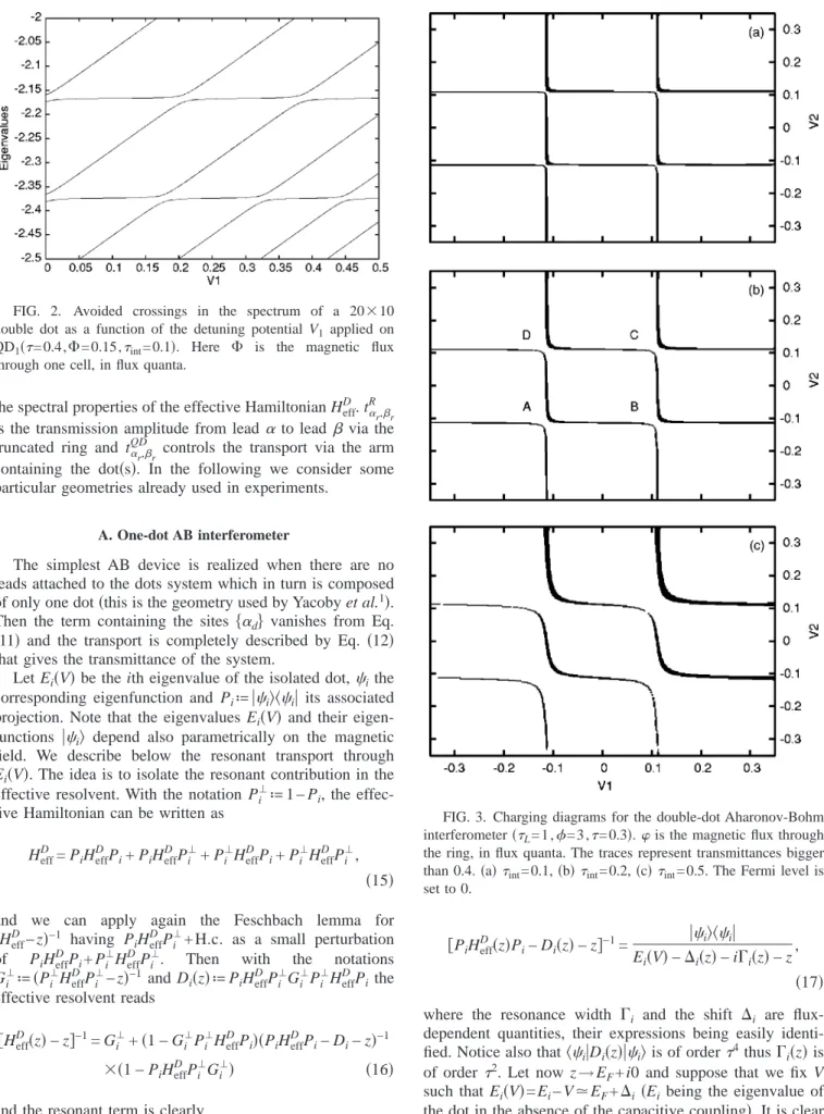
the dot in the absence of the capacitive coupling兲. It is clear FIG. 2. Avoided crossings in the spectrum of a 20⫻10
double dot as a function of the detuning potential V1 applied on
QD1共=0.4,⌽=0.15,int= 0.1兲. Here ⌽ is the magnetic flux
through one cell, in flux quanta.
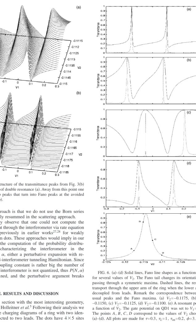
FIG. 3. Charging diagrams for the double-dot Aharonov-Bohm interferometer共L= 1 ,=3,=0.3兲. is the magnetic flux through
the ring, in flux quanta. The traces represent transmittances bigger than 0.4.共a兲int= 0.1,共b兲int= 0.2,共c兲int= 0.5. The Fermi level is
that the main contribution in 共16兲 comes from 关PiHeff
D共z兲P i
− Di共z兲−z兴−1since Gi⬜stays bounded and the other terms are
of O共2兲. The denominator of 关P
iHeff
D共z兲P
i− Di共z兲−z兴−1
re-duces to resonance width⌫iwhich compensates the
multipli-cative factor2 from the numerator of t ␣r,r
QD . This behavior
induces a peak in t␣
r,r
QD and hence in the total transmittance
across the ring. With these considerations we conclude that for weak ring-dot coupling, whenever V comes close to
EF− Ei for some Ei the transmittance can be written in the
form t␣ r,r QD = 2i L 22sin kG ␣r,0m R G 0n,r R e i共m−n兲具m兩 i典具i兩n典 Ei− V −⌬i− EF− i⌫i +O共2兲. 共18兲 Equation共18兲 is a Breit-Wigner-type formula and gives the transmittance between the leads via the quantum dot, as mea-sured in Refs. 1–3. A similar formula was obtained by Hack-enbroich and Weidenmüller for a continuous model.12,13 They supposed that Eiis flux independent, which is true only
at low magnetic fields and small dots. This assumption per-mits an analytical discussion of the flux-dependence of t␣
r,r QD
. As we have said, here we shall not neglect the effect of the magnetic field on the dot levels. We also point out that the one resonance form for the dot transmittance was obtained here starting from a many-level description of the dot. The rigorous argument for using from the beginning this simpli-fied form is that after subtracting the resonant term from the effective resolvent the remainder is nonsingular and small.
B. AB interferometer with a coherent double dot When HDdescribes two coupled dots embedded in
differ-ent arms of the ring connected to two leads共see Fig. 1兲 we recover the setup of Holleitner et al.5 In the absence of the lead-dot coupling Eqs. 共13兲 and 共14兲 give no contribution thus we are left only with Eq. 共12兲. For the simplicity of writing we shall denote G␣
r,0m
R ªG
␣r,m
R and
m−m⬘ªmm⬘.
Since G␣R = 0 in this case the conductance has the form
g␣= 4L44sin2k兩eiabG ␣a R G ab DG b R + eia⬘b⬘G ␣a⬘ R Ga ⬘b⬘ D Gb ⬘ R + eiab⬘G ␣a R G ab⬘ D Gb ⬘ R + eia⬘bG ␣a⬘ R Ga ⬘b D GbR兩2. 共19兲 We remark that the terms GaD⬘band GabD⬘connect points that belong to different dots. The effective Hamiltonian in this case is HeffD共z兲 = HD−2
兺
m,m⬘ e−imm⬘G m,m⬘ R 共z兲兩m典具m⬘
兩. 共20兲 As in the preceding section, we are interested in discussing the resonant transport in terms of the spectral properties of the coupled dots system. Since the double-dot HamiltonianHD depends parametrically on the capacitive couplings
V1, V2 we denote its eigenvalues and eigenfunctions by
Ei共V1, V2兲 andi共V1, V2兲. The main point is that for suitable pairs兵V1, V2其 one can bring Ei共V1, V2兲 close to Ej共V1, V2兲 for
j = i + 1. This is due to the spectral properties of detuned dots.
Let us remind here that the detuning consists in applying an additional gate potential to one dot while keeping the other gate voltage fixed. In Fig. 2 we show the spectrum of the detuned double dot共10⫻10 sites on each dot兲 as a function of the detuning potential V1 applied on the first dot, for a fixed value of int. For simplicity the undetuned dot is not capacitively coupled thus V2= 0. Obviously, one-half of the spectrum shifts linearly in V1. The remaining eigenvalues depend weakly on V1, excepting some points of avoided crossings. As long asint⫽0 there are no crossings between eigenvalues共on the contrary, as shown in Fig. 2 we rather have avoided crossings兲. Moreover, by perturbation theory, near avoided crossings the distance between eigenvalues is of orderint. This behavior of eigenvalues as functions of V1 and V2 is due to the fact that, roughly speaking, half of the eigenvalues belong to QD1, the other half to QD2. As a con-sequence, when V1, V2 are tuned such that both Ei共V1, V2兲 and Ej共V1, V2兲 are near and moreover close to the Fermi level we expect that both dots will transmit. Clearly one can study the tunneling through one eigenvalue following the same FIG. 4. The effects of the interdot coupling int on the electronic transmittance of a
double-dot Aharonov-Bohm interferometer at fixed mag-netic flux=3. The same gate potential V is ap-plied on each dotL= 1 ,=0.5. Full line, int= 1;
long dashed line,int= 0.5; dashed line,int= 0.2;
dotted line, int= 0 共transport is strongly
steps as in the analysis of a single-dot case. The interesting situation is however the one in which the resonant tunneling involves both eigenvalues. In the following we show how this appears formally at the level of GD. To this end let us
introduce the two-dimensional projection PijªPi+ Pj, Pk
being the projection associated to the eigenvalue Ek共V1, V2兲 with k = i , j for i and j fixed. We shall also use the notation
Pij⬜ª1−Pij. Then PijHeff DP ij ⬜+ H.c. is a perturbation 关of O共2兲兴 to P ijHeff DP ij+ Pij⬜Heff DP ij
⬜and by the Feschbach lemma for GeffD one has
GeffD =共Pij⬜HeffDPij⬜− z兲−1+关H˜effD共z兲 − z兴−1+O共4兲, 共21兲 with H ˜ eff D共z兲ª P ijHeff D共z兲P ij− PijHeff D Pij⬜共Pij⬜Heff D Pij⬜− z兲−1 ⫻Pij⬜Heff DP ij¬ H D共z兲 − D ij共z兲. 共22兲
As in the case of a single dot the first term in 共21兲 is small when z→EF+ i0 and the gate voltages are chosen such that the resonant condition is fulfilled at least around one of the two eigenvalues Ek共V1, V2兲. Then the last step to be done is to write the Dyson expansion of 共H˜effD− z兲−1 taking
PiH˜effDPj+ H.c.ªV as a perturbation of the 2⫻2 diagonal matrix PiH˜eff
DP
i+ PjH˜eff
DP j,
G˜effD = G˜ij,effD 共z兲 + G˜ij,effD 共z兲VG˜ij,effD + ¯ , 共23兲 where the unperturbed resolvent G˜ij,effD ¬G共i兲+ G共 j兲 has the form G˜ij,eff D 共z兲 = 兩i典具i兩 Ei共V1,V2兲 − ⌬i共z兲 − i⌫i共z兲 − z + 兩j典具j兩 Ej共V1,V2兲 − ⌬j共z兲 − i⌫j共z兲 − z . 共24兲
The indices i , j were explicitly written for the unperturbed operator 共we did not introduce another notation兲. Thus, we have here two resonances of widths⌫i,⌫j关their expressions
are complicated but easy to obtain from共22兲兴. It is clear that as long as the dots are coupled Ei共V1, V2兲⫽Ej共V1, V2兲 thus the two resonances come close but do not cross. Indeed, if for some V1, V2the first term in 共24兲 behaves like 1/⌫i the
denominator of the second term isint+共⌬i−⌬j兲−i⌫jthus the
resonant condition is not strictly achieved. Let us write ex-plicitly the second term from the Dyson expansion 共23兲. Since V is off-diagonal one is left with
G˜ij,effD 共z兲VG˜ij,effD 共z兲 = 兩i典具j兩Heff D
+ Dij共z兲兩i典具j兩 + H.c.
„Ei共V1,V2兲 − ⌬i共z兲 − i⌫i共z兲 − z… · „Ej共V1,V2兲 − ⌬j共z兲 − i⌫j共z兲 − z…
. 共25兲
Looking at 共20兲 and 共22兲 one notes that the numerator is quadratic inas well as the widths of the resonances⌫i,⌫j. Thus the perturbative expansion共23兲 cannot be used in the case of decoupled dots since Eiand Ejcan cross, the
imagi-nary parts of the resonances are equal ⌫i=⌫j=⌫ and G
˜ ij,eff D VG˜
ij,eff
D behaves also like 1 /⌫. However here we deal
with coupled dots and as long as int⬎2 the Dyson series 共23兲 converges and 共19兲 becomes 共omitting the indexes i, j and eff in G˜ij,effD 兲
g␣= 4L4sin2k兩2关eiabG ␣a R G˜abDGbR+ eia⬘b⬘G ␣a⬘ R G ˜ a⬘b⬘ D GbR⬘ + eiab⬘G ␣a R G˜abD⬘GRb⬘+ eia⬘bG ␣a⬘ R G˜aD⬘bGRb+O共2兲兴兩2. 共26兲 The last formula allows a discussion of the interferometer properties of the device. The first two terms represent the direct tunneling through the upper and lower dot, while the terms containing G˜ab ⬘ D and G˜a ⬘b D
describe paths in which the electron tunnels from one dot to the other before being trans-mitted in the leads. At small interdot coupling the cross prod-ucts 具a兩k典具k兩b
⬘
典, 具a⬘
兩k典具k兩b典, 具a兩j典具j兩b典, and具a
⬘
兩i典具i兩b⬘
典 are expected to be small so that we can write关keeping only the first two terms from the right-hand side of Eq.共26兲兴 g␣= 4L4sin2k
冏
2冉
e iabG ␣a R 具a兩 i典具i兩b典Gb R Ei共V1,V2兲 − ⌬i− i⌫i− z + eia⬘b⬘G ␣a⬘ R 具a⬘
兩j典具j兩b⬘
典Gb⬘ R Ej共V1,V2兲 − ⌬j− i⌫j− z冊
+R冏
2 , 共27兲 whereR collect all the other paths within the interferometer that give smaller contributions. Equation共27兲 will help us to discuss the numerical results from the next section.One may notice that in the above analysis the spectral properties of the truncated ring do not appear in an essential way in the problem. This could be anticipated from the be-ginning since it is the double-dot system that controls the tunneling events. At the formal level, this fact is revealed only by using the Feschbach formula.
We mention that our Eqs.共12兲–共14兲 and 共18兲 are similar to the ones obtained previously by Hackenbroich and Weidenmüller11,12 by a scattering theory approach, in the case of a single dot embedded in a ring connected to two leads. Here we gave an alternative calculation in terms of the Green functions rather than using the S matrix and we gen-eralized the discussion beyond the single-dot case. An
advan-tage of our approach is that we do not use the Born series which is formally resummed in the scattering approach.
Let us finally observe that one could not compute the tunneling current through the interferometer via rate equation methods used previously in earlier works27,28 for weakly coupled quantum dots. These approaches would imply in our problem either the computation of the probability distribu-tion P共N,␣兲 characterizing the interferometer in the N-particle state ␣, either a perturbative expansion with re-spect to the lead-interferometer tunneling Hamiltonian. Since the lead-ring coupling constant is rather big the number of electrons in the interferometer is not quantized, thus P共N,␣兲 is not well-defined, and the perturbative argument breaks down.
III. RESULTS AND DISCUSSION
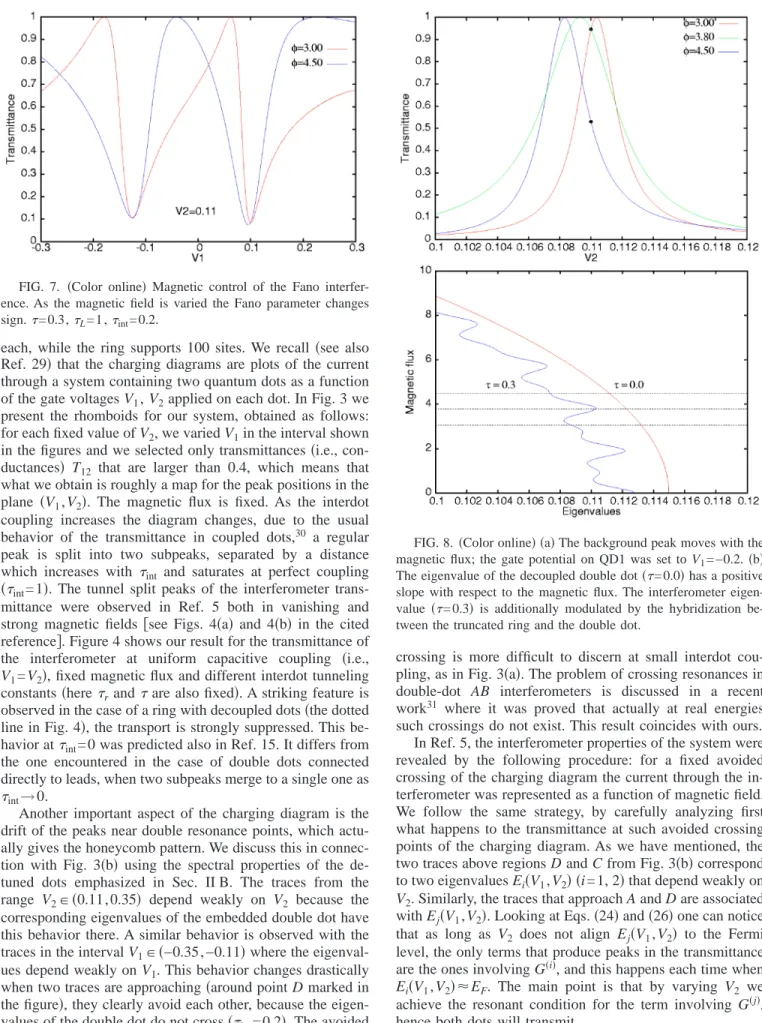
We start this section with the most interesting geometry, the one used by Holleitner et al.5Following their analysis we first look for the charging diagrams of a ring with two iden-tical dots connected to two leads. The dots have 4⫻5 sites FIG. 5. The structure of the transmittance peaks from Fig. 3共b兲 around the points of double resonance共a兲. Away from this point one has distinct sharp peaks that turn into Fano peaks at the avoided crossing points共b兲.
FIG. 6. 共a兲–共d兲 Solid lines, Fano line shapes as a function of V1 for several values of V2. The Fano tail changes its orientation by
passing through a symmetric maxima. Dashed lines, the resonant transport through the upper arm of the ring when the lower arm is decoupled from leads. Remark the correspondence between the usual peaks and the Fano maxima. 共a兲 V2= −0.1175, 共b兲 V2=
−0.1150,共c兲 V2= −0.1125,共d兲 V2= −0.1100.共e兲 A resonant peak as
a function of V2. The gate potential on QD1 was set to V1= −0.2. The points A , B , C , D correspond to the values of V2chosen in
each, while the ring supports 100 sites. We recall共see also Ref. 29兲 that the charging diagrams are plots of the current through a system containing two quantum dots as a function of the gate voltages V1, V2applied on each dot. In Fig. 3 we present the rhomboids for our system, obtained as follows: for each fixed value of V2, we varied V1in the interval shown in the figures and we selected only transmittances共i.e., con-ductances兲 T12 that are larger than 0.4, which means that what we obtain is roughly a map for the peak positions in the plane 共V1, V2兲. The magnetic flux is fixed. As the interdot coupling increases the diagram changes, due to the usual behavior of the transmittance in coupled dots,30 a regular peak is split into two subpeaks, separated by a distance which increases with int and saturates at perfect coupling 共int= 1兲. The tunnel split peaks of the interferometer trans-mittance were observed in Ref. 5 both in vanishing and strong magnetic fields关see Figs. 4共a兲 and 4共b兲 in the cited reference兴. Figure 4 shows our result for the transmittance of the interferometer at uniform capacitive coupling 共i.e.,
V1= V2兲, fixed magnetic flux and different interdot tunneling constants共hererandare also fixed兲. A striking feature is
observed in the case of a ring with decoupled dots共the dotted line in Fig. 4兲, the transport is strongly suppressed. This be-havior atint= 0 was predicted also in Ref. 15. It differs from the one encountered in the case of double dots connected directly to leads, when two subpeaks merge to a single one as int→0.
Another important aspect of the charging diagram is the drift of the peaks near double resonance points, which actu-ally gives the honeycomb pattern. We discuss this in connec-tion with Fig. 3共b兲 using the spectral properties of the de-tuned dots emphasized in Sec. II B. The traces from the range V2苸共0.11,0.35兲 depend weakly on V2 because the corresponding eigenvalues of the embedded double dot have this behavior there. A similar behavior is observed with the traces in the interval V1苸共−0.35,−0.11兲 where the eigenval-ues depend weakly on V1. This behavior changes drastically when two traces are approaching共around point D marked in the figure兲, they clearly avoid each other, because the eigen-values of the double dot do not cross共int= 0.2兲. The avoided
crossing is more difficult to discern at small interdot cou-pling, as in Fig. 3共a兲. The problem of crossing resonances in double-dot AB interferometers is discussed in a recent work31 where it was proved that actually at real energies such crossings do not exist. This result coincides with ours. In Ref. 5, the interferometer properties of the system were revealed by the following procedure: for a fixed avoided crossing of the charging diagram the current through the in-terferometer was represented as a function of magnetic field. We follow the same strategy, by carefully analyzing first what happens to the transmittance at such avoided crossing points of the charging diagram. As we have mentioned, the two traces above regions D and C from Fig. 3共b兲 correspond to two eigenvalues Ei共V1, V2兲 共i=1, 2兲 that depend weakly on
V2. Similarly, the traces that approach A and D are associated with Ej共V1, V2兲. Looking at Eqs. 共24兲 and 共26兲 one can notice that as long as V2 does not align Ej共V1, V2兲 to the Fermi level, the only terms that produce peaks in the transmittance are the ones involving G共i兲, and this happens each time when
Ei共V1, V2兲⬇EF. The main point is that by varying V2 we achieve the resonant condition for the term involving G共j兲, hence both dots will transmit.
FIG. 7. 共Color online兲 Magnetic control of the Fano interfer-ence. As the magnetic field is varied the Fano parameter changes sign.=0.3, L= 1 ,int= 0.2.
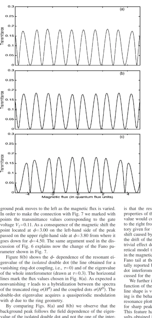
FIG. 8.共Color online兲 共a兲 The background peak moves with the magnetic flux; the gate potential on QD1 was set to V1= −0.2.共b兲
The eigenvalue of the decoupled double dot共=0.0兲 has a positive slope with respect to the magnetic flux. The interferometer eigen-value 共=0.3兲 is additionally modulated by the hybridization be-tween the truncated ring and the double dot.
In Fig. 5 we show a detail from the charging diagram in Fig. 3共b兲, taken in the neighborhood of almost crossing points A and B. In contrast to the usual picture with sharp peaks here we observe关Fig. 5共a兲兴 an asymmetric large tail of the peaks, which shows that in this regime the interferometer acts as a Fano system. This happens because one dot共QD2兲 is always set to a resonance thus the corresponding arm of the ring is free, providing the continuum component for the interference. Formally this is easily understood by looking at Eq.共27兲, because the second term is always large enough and interfere with a quantity 共the first term兲 that increases as
Ei共V兲 approaches the Fermi level. The Fano regime
disap-pears quickly as we tune QD2 away from resonance, the picture of separate peaks being recovered关Fig. 5共b兲兴.
In Figs. 6共a兲–6共d兲 the solid lines are plots of the transmit-tance as a function of V1when V2 is set close to a resonant value. Remark the sudden drop of the peak after the resonant point and the Fano dips. The latter are actually located in the avoided crossing region, which explains the small transmit-tance there. Moreover, the asymmetric tail changes its orien-tation as V2 is slightly varied, i.e., the Fano parameter sign changes. Following Kobayashi et al.7 we shall call this fea-ture the electrostatic control of the Fano asymmetric line. In order to explain this observation we must look at the two paths that are involved in the interference. The first contri-bution comes from the resonant tunneling through the upper dot and is given as dashed lines in Figs. 6共a兲–6共d兲 共the plots were obtained by decoupling the lower arm of the ring from the leads兲. In this case there is no interference and one gets the usual resonant peaks. The second contribution is due to the background transmittance of the lower arm when V2 is
set close to a resonance and the upper arm does not transmit. We illustrate this component of transport in Fig. 6共e兲 which shows a single peak that appears by varying V2 when V1 is far away from resonant values. The points A , B , C , D mark the magnitude of the background for four values of V2. Clearly, as V1approaches the resonant points the interference becomes possible and the Fano lines appear. By inspecting each of Figs. 6共a兲–6共d兲 in connection with Fig. 6共e兲 one gets a description of the line shape for different pairs of V1, V2. As long as the transmittance values of the two contributions are located on the same side of their corresponding peaks the interference is constructive and the Fano line increase up to a maximum which coincides with the resonant peak of the upper arm. In contrast, when V1, V2are chosen such that the transmittance values are located on different sides of the peaks the two path interfere destructively and the Fano line drops to a dip. In particular, for V2 fixed the dips will be located on the same side of the peaks, thus the Fano param-eter conserve its sign. The appearance of Fano effect in in-terferometers with embedded dots was also discussed in a simple共exactly solvable兲 model in Ref. 32, without consid-ering the interdot coupling or emphasizing the electrostatic control of the Fano line shape.
In the above discussion the magnetic flux was fixed and we have varied V2, emphasizing the sensitivity of the Fano interference on this parameter. Figure 7 shows that the shape of the Fano line can be equally controlled by varying the magnetic flux, while keeping V2fixed. Indeed, asincreases from 3.00 to 4.50 the asymmetric tail changes its orientation. This effect originates in the field dependence of the dot lev-els which leads in turn to a shift of the background peak. Indeed from Fig. 8共a兲 one notices at once that the back-FIG. 9. The sharpness of the Fano resonances共a兲 and the phase of the transmittance through the interferometer共b兲, as a function of the interdot coupling, full line, int= 0.05; dashed line, int= 0.15;
dotted line,int= 0.3. At weak
cou-pling the phase increases rapidly by 2 while for stronger coupling it increases smoothly by 2 along a Fano resonance. The parameters used are V2= −0.110,=3,
ground peak moves to the left as the magnetic flux is varied. In order to make the connection with Fig. 7 we marked with points the transmittance values corresponding to the gate voltage V2= 0.11. As a consequence of the magnetic shift the point located at = 3.00 on the left-hand side of the peak passed on the upper right-hand side at= 3.80 from where it goes down for= 4.50. The same argument used in the dis-cussion of Fig. 6 explains now the change of the Fano pa-rameter shown in Fig. 7.
Figure 8共b兲 shows the- dependence of the resonant ei-genvalue of the isolated double dot共the line obtained for a vanishing ring-dot coupling, i.e.,= 0兲 and of the eigenvalue of the whole interferometer共drawn at= 0.3兲. The horizontal lines mark the flux values chosen in Fig. 8共a兲. As expected a nonvanishingleads to a hybridization between the spectra of the truncated ring共HR兲 and the coupled dots共HD兲. The
double-dot eigenvalue acquires a quasiperiodic modulation withdue to the ring geometry.
By comparing Figs. 8共a兲 and 8共b兲 we observe that the background peak follows the field dependence of the eigen-value of the isolated double dot and not the one of the inter-ferometer eigenvalue. The physical meaning of this behavior
is that the resonant transport is controlled by the spectral properties of the embedded dots. If the interferometer eigen-value would control the peak position this one should move to the right from= 3.00 to= 3.80, according to the trajec-tory given for= 0.3. Clearly this is not the case and, up to a shift caused by the real part of the resonance the peak obeys the drift of the isolated eigenvalue. We stress that this non-trivial effect described above cannot be captured by a theo-retical model that neglects the spectral properties of the dot in the magnetic field. The direction change of the asymmetric Fano tail at the variation of magnetic field was experimen-tally reported by Kobayashi et al.7in the the case of a one-dot interferometer. We believe that the effect we just dis-cussed for the two-dots interferometer is similar.
We further investigate the behavior of the Fano peaks as a function of the interdot coupling. Figure 9共a兲 shows that the line shape is very sensitive to this parameter. More interest-ing is the behavior of the interferometer phase along a Fano resonance plotted in Fig. 9共b兲. For weak coupling 共and hence for sharp peaks兲 the phase shows a rapid increase by 2. This feature has some connection with the experimental re-sults obtained in a single dot interferometer by Kobayashi et
al.7They reported an increase of 2for the phase of the AB FIG. 10. The in-phase Aharonov-Bohm oscil-lations of the transmittance assigned to the Fano dips from the region A , B , C, and D in Fig. 3共b兲.
oscillations 共we present instead the phase of the transmit-tance兲. In our case the second dot is set to a resonance so it acts as a free arm of the ring, from where the similarity with the one-dot interferometer. By increasing int the phase be-comes a smooth function of V1.
We now address the problem of AB oscillations. It is clear that they are to be observed if both dots are close to reso-nance, meaning that the gate voltages V1, V2 are suitably tuned near some eigenvalues of the double dot. The delicate point is that the eigenvalues depend on the magnetic flux through the ring so that for different fluxes one needs differ-ent resonant values for V1, V2. Otherwise stated, the rhom-boids move with 共not shown兲. We found that for small
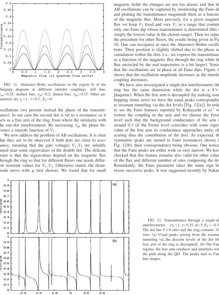
magnetic fields the changes are not too drastic and that the AB oscillations can be captured by monitoring the Fano dip and plotting the transmittance magnitude there as a function of the magnetic flux. More precisely, for a given magnetic flux we keep V2 fixed and vary V1 in a range that contains only one Fano dip whose transmittance is determined共this is simply the lowest value in the chosen range兲. Then we repeat the procedure for other fluxes, the results being given in Fig. 10. One can recognize at once the Aharonov-Bohm oscilla-tions. Their position is slightly shifted due to the phase ac-cumulation within the dots共i.e., we express the transmittance as a function of the magnetic flux through the ring while the flux encircled by the real trajectories is a bit larger兲. Notice that the oscillations are in phase at all Fano dips. Figure 11 shows that the oscillation amplitude increases as the interdot coupling decreases.
We have also investigated a single-dot interferometer共the ring has the same dimension while the dot is a 8⫻9 plaquette兲. When the free arm is decoupled 共by making some hopping terms zero兲 we have the usual peaks corresponding to resonant tunneling via the dot levels关Fig. 12共a兲兴. In order to see the Fano features reported by Kobayashi et al.7 we restore the coupling to the arm and we choose the Fermi level such that the background conductance of the arm is around 0.3 共if the Fermi level coincides with some eigen-value of the free arm its conductance approaches unity, ob-scuring thus the contribution of the dot兲. As expected, the symmetric peaks are turned to Fano resonances shown in Fig. 12共b兲, their correspondence being obvious. One notices that the Fano peaks are either wide or very narrow. We have checked that this feature remains also valid for other values of the flux and different number of sites composing the dot. Remarkably, the Fano parameter takes the same sign be-tween succesive peaks. It was suggested recently by Nakan-FIG. 11. Aharonov-Bohn oscillations in the region D of the
charging diagram at different interdot couplings, full line, int= 0.25; dashed line, int= 0.2; dotted line,int= 0.15. Other
pa-rameters are tL= 1 ,=0.3, EF= 0.
FIG. 12. Transmittance through a single-dot interferometer 共L= 1 ,=0.35,=5,EF= −0.5兲. The dot has 9⫻8 sites and the ring contains 100 sites. 共a兲 Usual peaks arising from the resonant tunneling via the discrete levels of the dot共the free arm of the ring is decoupled兲. 共b兲 The Fano regime, the free arm conducts and interferes with the path along the QD. The peaks turn to Fano line shapes.
ishi et al.33 that this feature relates to the correlations be-tween the narow and wide peaks.
IV. CONCLUSIONS
The main aim of this paper was to present in a unified formalism the basic properties of Aharonov-Bohm interfer-ometers with coupled quantum dots. By combining the Landauer-Büttiker approach and the Feschbach formula we studied the transport properties of the interferometer in terms of the spectral properties of the embedded dots. Our method involves only Green functions and can be viewed as an al-ternative to the scattering theoretical approach. In the case of an interferometer with two coupled QD共one QD in each arm of the ring兲 we give a formula 关Eq. 共27兲兴 which emphasizes the resonant tunneling process through a given discrete level from the dots共we recall that along the paper we have con-sidered many-level dots兲.
Numerical simulations reproduce the stability charging diagrams of two-dot AB interferometer reported in the ex-periments of Holleitner et al.5A careful analysis of the al-most crossing points of the diagram lead us to several inter-esting results which are summarized in what follows. When the magnetic field is fixed and one dot is set to resonance the interferometer transmittance shows Fano line shapes as a function of the gate voltage applied to the other dot. This
corroborates with the results of Kubala and König32obtained in an exactly solvable one-site model and shows clearly the coherent feature of the transport through the system. We em-phasized and explained the sensitivity of the Fano tail to the gate potential on the second dot.
As we have said, our model includes the effect of the magnetic field on the dot levels. It turned out that this effect explains the change of the asymmetric tail as the magnetic flux is varied. It would be of great interest to probe experi-mentally this latter aspect. The transmittance assigned to the Fano dips shows Aharonov-Bohm oscillations, in full agree-ment with the observations of Holleitner et al.5The influence of the various coupling constants was identified. Finally we reproduced the results of Kobayashi et al.7
The analysis of the 4-lead geometry in view of the very recent results reported in the study by Sigrist et al.6is much more complex and requires further investigation.
ACKNOWLEDGMENTS
This work was supported by Grant CNCSIS and Roma-nian Programme for Fundamental Research. V.M. acknowl-edges support from the NATO-TUBITAK and the Romanian Ministry of Education and Research under CERES contract. B.T. acknowledges the support of TUBITAK, NATO-SfP, MSB-KOBRA, and TUBA. The authors are very grateful to Ulrich Wulf for many valuable discussions.
1A. Yacoby, M. Heiblum, D. Mahalu, and Hadas Shtrikman, Phys.
Rev. Lett. 74, 4047共1995兲.
2A. L. Yeyati and M. Büttiker, Phys. Rev. B 52, R14360共1995兲. 3R. Schuster, E. Bucks, M. Heiblum, D. Mahalu, V. Umanski, and
Hadas Shtrikman, Nature共London兲 385, 417 共1997兲.
4E. Bucks, R. Schuster, M. Heiblum, D. Mahalu, and V. Umanski,
Nature共London兲 391, 871 共1998兲.
5A. W. Holleitner, C. R. Decker, H. Qin, K. Eberl, and R. H. Blick,
Phys. Rev. Lett. 87, 256802共2001兲; A. W. Holleitner, H. Qin, K. Eberl, and J. P. Kotthaus, Physica E共Amsterdam兲 12, 774 共2002兲.
6M. Sigrist, et al., Phys. Rev. Lett. 93, 066802共2004兲.
7Kensuke Kobayashi, Hisashi Aikawa, Shingo Katsumoto, and
Ya-suhiro Iye, Phys. Rev. Lett. 88, 256806共2002兲; Phys. Rev. B 68, 235304共2003兲.
8U. Fano, Phys. Rev. 124, 1866共1961兲.
9J. U. Nockel, and A. D. Stone, Phys. Rev. B 50, 17415共1994兲. 10E. R. Racec and U. Wulf, Phys. Rev. B 64, 115318共2001兲. 11G. Hackenbroich and H. A. Weidenmüller, Phys. Rev. Lett. 76,
110共1996兲.
12G. Hackenbroich and H. A. Weidenmüller, Phys. Rev. B 53,
16379共1996兲.
13G. Hackenbroich, Phys. Rep. 343, 463共2001兲.
14J. König and Y. Gefen, Phys. Rev. B 65, 045316共2002兲. 15B. Kubala and J. König, Phys. Rev. B 67, 205303共2003兲. 16H. A. Weidenmüller, Phys. Rev. B 65, 245322共2002兲.
17O. Entin-Wohlman, A. Aharony, Y. Imry, Y. Levinson, and A.
Schiller, Phys. Rev. Lett. 88, 166801共2002兲.
18A. Aharony, O. Entin-Wohlman, B. I. Halperin, and Y. Imry,
Phys. Rev. B 66, 115311共2002兲.
19A. Aharony, O. Entin-Wohlman, and Y. Imry, Turk. J. Phys. 27,
299共2003兲.
20H. Feschbach, Ann. Phys.共N.Y.兲 5, 363 共1958兲. 21G. Nenciu, Rev. Mod. Phys. 63, 91共1991兲.
22V. Moldoveanu, A. Aldea, A. Manolescu, and M. Nita, Phys. Rev.
B 63, 045301共2001兲.
23A. Aldea, V. Moldoveanu, M. Nita, A. Manolescu, V.
Gudmunds-son, and B. Tanatar, Phys. Rev. B 67, 035324共2003兲.
24V. Moldoveanu, A. Aldea, and B. Tanatar, Phys. Rev. B 70,
085303共2004兲.
25H. D. Cornean, A. Jensen, and V. Moldoveanu, Report No.
mp-arc 04-71, available at http://www.ma.utexas.edu
26S. Datta, Electronic Transport in Mesoscopic Systems共Cambridge
University Press, Cambridge, 1995兲.
27F. Ramirez, E. Cota, and S. E. Ulloa, Phys. Rev. B 59, 5717
共1999兲.
28R. Ziegler, C. Bruder, and H. Schoeller, Phys. Rev. B 62, 1961
共2000兲.
29W. G. van der Wiel, S. De Franceschi, J. M. Elzerman, T.
Fujisawa, S. Tarucha, and L. P. Kouwenhoven, Rev. Mod. Phys. 75, 1共2003兲.
30F. R. Waugh, M. J. Berry, D. J. Mar, R. M. Westervelt, K. L.
Campman, and A. C. Gossard, Phys. Rev. Lett. 75, 705共1995兲.
31H. A. Weidenmüller, Phys. Rev. B 68, 125326共2003兲. 32B. Kubala and J. König, Phys. Rev. B 65, 245301共2002兲. 33T. Nakanishi, K. Terakura, and T. Ando, Phys. Rev. B 69, 115307