OPTIMAL BROADCAST ENCRYPTION
WITH FREE RIDERS
a thesis
submitted to the department of computer engineering
and the institute of engineering and science
of bilkent university
in partial fulfillment of the requirements
for the degree of
master of science
By
Murat Ak
September, 2006
I certify that I have read this thesis and that in my opinion it is fully adequate, in scope and in quality, as a thesis for the degree of Master of Science.
Assist. Prof. Dr. Ali Aydın Sel¸cuk(Advisor)
I certify that I have read this thesis and that in my opinion it is fully adequate, in scope and in quality, as a thesis for the degree of Master of Science.
Assist. Prof. Dr. ˙Ibrahim K¨orpeo˘glu
I certify that I have read this thesis and that in my opinion it is fully adequate, in scope and in quality, as a thesis for the degree of Master of Science.
Assist. Prof. Dr. Alper S¸en
Approved for the Institute of Engineering and Science:
Prof. Dr. Mehmet B. Baray Director of the Institute
ABSTRACT
OPTIMAL BROADCAST ENCRYPTION WITH FREE
RIDERS
Murat Ak
M.S. in Computer Engineering
Supervisor: Assist. Prof. Dr. Ali Aydın Sel¸cuk September, 2006
Broadcast encryption schemes allow a center to broadcast encrypted mes-sages so that each particular message can only be decrypted by a set of privileged receivers designated for it. The standard technique is to distribute keys to all re-ceivers at the beginning and to use only the necessary keys to encrypt the message for each particular broadcast. The number of encryptions needed constitutes the transmission cost in broadcast encryption schemes. The most efficient scheme in terms of transmission cost published so far is the subset difference (SD) scheme. It is possible to reduce the transmission overhead of a broadcast encryption scheme by allowing a number of free riders to be able to decrypt the message although they are not privileged. However, unless the free riders are chosen cleverly, the cost may even increase. In this thesis, we deal with the problem of choosing a given number of free riders effectively to reduce the transmission overhead in SD scheme. We first present three greedy algorithms. First algorithm has a fast execution, the second one is slower but has lower transmission overhead, and the last one has a trade-off between running time and transmission cost. Then we present two algorithms which find the minimum transmission overhead possible given a free rider quota. The experiments we conduct show that the transmission cost can be significantly reduced.
Keywords: Broadcast Encryption, Free Riders. iii
¨
OZET
MUAF KULLANICILARLA EN UYGUN YAYIN
S
¸ ˙IFRELENMES˙I
Murat Ak
Bilgisayar M¨uhendisli˘gi, Y¨uksek Lisans Tez Y¨oneticisi: Assist. Prof. Dr. Ali Aydın Sel¸cuk
Eyl¨ul, 2006
Yayın ¸sifreleme planları bir merkezin ¸sifreli mesajlar yayınlamasını sa˘glar. ¨Oyle ki herbir mesajı sadece o mesaj icin belirlenmi¸s imtiyazlı bir grup de¸sifre edebilir. Standart teknik en ba¸sta t¨um alıcılara anahtarlar da˘gıtıp herbir yayında mesajı sadece gerekli anahtarlarla ¸sifrelemektir. Yapılan ¸sifreleme sayısı g¨onderim mas-rafını olu¸sturmaktadır. Bu masraf bakımından ¸su ana kadar yayınlanmı¸s en iyi plan Altk¨ume Farkı (AF) planıdır. Bir yayın ¸sifreleme planında imtiyazlı olmayan bir takım alıcıların da yayını de¸sifre edebilmesine izin verilmesi suretiyle g¨onderim masrafının azaltılması m¨umk¨und¨ur. Fakat bunun i¸cin muaf kullanıcıların akıllıca se¸cilmesi gerekmektedir. Bu tez AF planında g¨onderim masrafını azaltmak i¸cin izin verilen sayıda muaf kullanıcının etkin olacak ¸sekilde se¸cilmesi problemini hedef almaktadır. ¨Oncelikle ¨u¸c adet haris algoritma sunuyoruz. Bunlardan birin-cisi hızlı ¸calı¸sma s¨uresine, ikincisi daha yava¸s ¸calı¸smasına kar¸sın daha az g¨onderim masrafına sahiptir. Sonuncusu ise bu iki unsur arasında dengeyi sa˘glamaktadır. Daha sonra belli bir muaf kullanıcı kotası verildi˘ginde asgari g¨onderim masrafına ula¸san iki algoritma sunuyoruz. Y¨ur¨utm¨u¸s oldu˘gumuz deneyler g¨ostermektedir ki g¨onderim masrafı b¨uy¨uk ¨ol¸c¨ude azaltılabilmektedir.
Anahtar s¨ozc¨ukler : Yayın S¸ifreleme, Muaf Kullanıcı. iv
Acknowledgement
I would like to express my gratitude to Dr. Ali Aydın Sel¸cuk for offering his valu-able time and support as my supervisor. I have learned a lot from his suggestions during this research. He also helped me to keep my interest all along.
I am grateful to Dr. ˙Ibrahim K¨orpeo˘glu and Dr. Alper S¸en for accepting to read and review this thesis.
I am also indebted to Kamer Kaya who helped me with the technical aspects of this research and gave inspirations for some of the algorithms.
I would like to thank the other members of Security Reading Group (SRG) who have been very gentle and friendly since the beginning.
I would like to express my gratitude and appreciation to my parents for their infinite love, support and guidance.
I acknowledge that TUBITAK (The Scientific and Technical Research Council of Turkey) supported this study under MSc. Scholarship program.
vi
Contents
1 Introduction 1
1.1 Related Work . . . 3
1.2 Problem Definition . . . 4
2 Free Rider Problem and SD Scheme 6 2.1 Notation and Subset Cover Framework . . . 6
2.2 Free Rider Assignment Problem . . . 8
2.2.1 Tree Scheme and f-Cover Algorithm . . . 11
2.2.2 The Complete Subtree Scheme . . . 11
2.2.3 CS with Optimal Free Rider Assignment . . . 12
2.3 The Subset Difference Scheme . . . 12
2.4 Definitions . . . 14
3 Greedy Algorithms 18 3.1 Top-Down Algorithm . . . 18
3.2 Bottom-Up Algorithm . . . 20 vii
CONTENTS viii
3.3 Hybrid Algorithm . . . 25
4 Optimal Free Rider Assignment for SD 26 4.1 The Optimization Algorithms . . . 26
4.1.1 The Basic Algorithm . . . 27
4.1.2 Improved Algorithm . . . 32
5 Experimental Results 37 5.1 Evaluation Parameters . . . 37
5.2 Implementation Issues . . . 38
5.3 Experiments . . . 39
5.3.1 Transmission Overhead Experiments . . . 39
5.3.2 Running Time Comparisons . . . 43
List of Figures
2.1 Subset Cover Example 1 . . . 8
2.2 Subset Cover Example 2 . . . 9
2.3 Level ordering . . . 15 2.4 SD Configuration . . . 15 3.1 Removal of a subset . . . 21 3.2 No profit . . . 22 3.3 Profit of 1 . . . 22 3.4 Profit of 2 . . . 23
5.1 Transmission costs with f = 2.0 . . . 39
5.2 Transmission costs with f = 1.6 . . . 40
5.3 Transmission costs with f = 1.34 . . . 40
5.4 Transmission costs with f = 1.231 . . . 41
5.5 Transmission costs with f = 1.143 . . . 41
5.6 Transmission costs with f = 1.067 . . . 42 ix
List of Tables
2.1 Preliminary Notation . . . 14
5.1 Running Times of the Algorithms . . . 44
Chapter 1
Introduction
Broadcast encryption is the process of sending a message to a set of receivers by encrypting it to guarantee that only a designated subset of the receivers is able to decrypt, preventing the others to decrypt. Idea of broadcast encryption main-tains a solution to the problem of secure communication over one way channels, specifically when a center has to communicate with a huge group of receivers. It has many applications but the most popular ones are content protection and media multicast over cable television or internet. Content protection is the act of preventing unauthorized copying of copyrighted CDs, DVDs, etc. In media mul-ticast, broadcast encryption is needed when a cable TV channel wants to restrict access to its programs to the subscribed users.
Broadcast encryption is usually done as follows: Receivers are given some symmetric keys at the beginning. For example, in cable TV scenario, these keys are burned into the set-top boxes in the devices of the customers. When the center is going to send a message, it encrypts the message with a master key, and encrypt this key with each of some selected keys among the ones that was given to the receivers, and broadcasts them together with the encrypted message. Upon a message arrival, a receiver is able to view the message if it has one of the keys that the center used.
The aim of the broadcast encryption schemes is to improve basically two 1
CHAPTER 1. INTRODUCTION 2
important evaluation parameters, the number of keys stored per receiver and the number of encryptions that the center do, referred as key storage and transmission overhead respectively. The complexities are usually in terms of the number of all receivers N , and the number of revoked users, r. These parameters will be explained in detail in Chapter 2.
In broadcast encryption, receivers are modelled as either stateless or dynamic. When we talk about stateless receivers, that means the keys assigned to the receivers do not change once they are given at the beginning. However, keys of dynamic receivers are changed while the system is running, which is called rekeying. This approach is mostly suitable for only the applications where most of the receivers are privileged. Therefore it is mostly used for rekeying when a key of a receiver is compromised. On the other hand, stateless receivers are appropriate for cable TV applications, because a program may not be subscribed by most of the customers, and since cable TV’s has thousands or millions of users, it is infeasible to rekey whenever a user is revoked. In this work, we deal with the stateless receiver case.
The thesis is organized as follows: In Chapter 2, we present the broadcast problem in detail and explain some of the early results. Then we review subset difference scheme which is the current state of the art in broadcast encryption. Then we present the preliminaries, definitions and notations to be used in our algorithms. In Chapter 3, we give three algorithms for the broadcast problem with free riders. Basically, first two algorithms are based on different greedy heuristics, and the last one is obtained by merging them. In Chapter 4, we propose two slightly different algorithms for optimal free rider assignment. Both algorithms are based on a dynamic programming approach. In Chapter 5, we give the experimental results comparing the performances of our algorithms. In chapter 6, we conclude our work by discussing our results.
CHAPTER 1. INTRODUCTION 3
1.1
Related Work
Two years after Berkovits [1] introduced the idea of broadcast encryption in 1991, Fiat and Naor [2] presented their model which is accepted as the first formal work and milestone in the topic. They introduced the resiliency concept, and defined k-resilient to be resilient to coalition of at most k users. Their best scheme required every receiver to store O(k log k log N ) keys and the center to broadcast O(k2log2k log N ) messages. The schemes published after this work assumed that
perfect resiliency is required and resiliency concept was no longer used. After this work, broadcast encryption became a heavily studied research area. In 1998, Luby and Staddon [3] studied the trade off between the transmission and storage costs and gave combinatorial bounds.
In the late nineties, Wallner et al. [5] and Wong et al. [6] independently pro-posed logical tree hierarchy (LKH) for secure internet multicast. LKH was not a broadcast encryption scheme at all, but its key distribution idea was very useful for broadcast encryption. The idea was to relate the receivers with the leaves of a tree, associate a unique key to each node of the tree and give a receiver the keys of the nodes on the path from the corresponding leaf to the root. With this approach, key storage complexity became logarithmic in terms of the number of receivers, O(log N ), which was called as log-key storage restriction later.
In [7], which is the second milestone of broadcast encryption research, Naor, Naor and Lotspiech proposed two schemes, complete subtree (CS) and subset difference (SD). In fact, CS scheme was summarizing the current state of the art before SD scheme. It was actually a specific case of the scheme of Abdalla et al. [4] where redundancy is 0. CS scheme had O(log N ) key storage and O(r log N/r) transmission cost. What they did in SD scheme was to decrease the transmission overhead to O(log r) at the expense of increasing the key storage to O(log2N ). SD scheme was the best scheme by that time, and most of the new schemes proposed until today are still based on the SD scheme.
CHAPTER 1. INTRODUCTION 4
was proposed by Halevy and Shamir in [8]. Optimized LSD has a transmis-sion overhead of complexity O(log N log log N ) and key storage of complexity O(r log log N ). Later, Goodrich, Sun and Tamassia [10] introduced stratified subset difference (SSD) scheme, which has O(log r) transmission overhead and O(log N ) key storage complexity. A detailed analysis of [2, 7, 8] can be found in [9].
The idea of allowing some free riders to get better performance, was introduced by Abdalla, Shavitt and Wool [4] in 1999. This work was also the first to adapt the key distribution idea of LKH scheme to broadcast encryption. They investigated efficient usage of free riders in depth and figured out basic intuition about effective assignment of free riders.
Although allowing free riders is a useful approach, surprisingly, it was not used since [4] until Ramzan and Woodruff [19] recently proposed an algorithm which optimally chooses which revoked users to be allowed to be free riders to get minimal transmission overhead in CS scheme. Their algorithm was based on a dynamic programming approach, which decides the free rider assignment positions in subtrees in a tree recursively in a bottom-up fashion.
1.2
Problem Definition
Most of the work published so far has the following restriction: A message can be decrypted by privileged users but it cannot be decrypted by any other user even by coalitions of them. We call this restriction as the exact cover restriction. This level of security is certainly useful for applications which transfer critical data such as the ones used by military or intelligence agencies but especially commercial applications like TV broadcasts do not strictly need such a tight security. In fact, loosening this restriction may be useful by reducing the traffic of the network.
In the literature, free riders are defined as the receivers who are not privileged but are able to decrypt the message. Allowing free riders is useful because the transmission costs of the possible privileged receiver subsets are not same and
CHAPTER 1. INTRODUCTION 5
when the system have the chance to change the privileged subset slightly it will probably find a lower-cost subset which covers the original one and not much larger than it.
The problem we address in this thesis is how to minimize the transmission overhead by cleverly choosing a given number of free riders in subset difference scheme. The same problem was investigated and solved for complete subtree (CS) scheme in [19] by Ramzan and Woodruff. However, the subset difference (SD) scheme is the base scheme for the most efficient schemes today such as LSD [8] and SSD [10]. Therefore, the problem of optimally choosing the free riders should be solved for SD to get the best scheme that allows free riders.
In order to understand the free rider problem and to see its advantage, we need to know the subset structure used by the broadcast encryption schemes. We explain the subset cover framework in Section 2.1. Then we will explain the free rider assignment problem in detail in Section 2.2. Afterwards, we treat the free rider problem for SD scheme.
Chapter 2
Free Rider Assignment Problem
and SD Scheme
In this chapter, we first give the preliminary notation and Subset Cover frame-work. Then we explain the research problem of the thesis. Then we discuss the schemes before SD in detail and we explain the SD scheme. We finish the chapter by giving some definitions needed for our algorithms in the next chapters.
2.1
Notation and Subset Cover Framework
We denote the set of all users by U , with |U | = N . The set of revoked users for a particular broadcast is denoted by R, with |R| = r. The aim of the center is to send a message M encrypted by some keys to all users such that only the users in U \R can decrypt the ciphertext and get M .
Throughout this thesis, we will stick to the subset cover framework of [7], which formalizes the design process of a broadcast encryption scheme by explicitly defining the common properties and steps of every broadcast encryption scheme. In this framework, a collection S is defined first.
CHAPTER 2. FREE RIDER PROBLEM AND SD SCHEME 7
S = {Si|Si ⊆ U }
Then, every subset Si is associated with a key Ki and this key is given to
all receivers in Si. Upon a broadcast need, given the revoked user set R, an
algorithm Cover finds a set C (for cover) of the subsets such that
U \R ⊆S Si ∈ C
Then the message M is encrypted |C| times separately with the keys of the subsets in C. The minimum cardinality C is the optimal cover denoted by Copt. Any
algorithm Cover is aimed to find a C as small as possible.
Any broadcast encryption scheme using the formulation of subset cover frame-work, has to have three components.
• A Key Distribution Algorithm. This is the algorithm that defines the subsets. Once the subsets are defined, each subset is assigned a different key.
• A Covering Algorithm. First it chooses a session key, K. Then runs the Cover algorithm to find the cover, which is the set of subsets whose union covers the privileged subset of receivers. Finally it encrypts K with the keys of the subsets found by the Cover algorithm. Then, it sends the ID’s (i’s) of the subsets, encrypted session keys (E1
Ki(K)’s) and the message
M encrypted with K, (E2
K(M )) as the ciphertext.
• A Decryption Algorithm. Upon a message arrival to a receiver u, it finds whether any subsets that includes it is in the cover and if so, it extracts and decrypts E1
Ku(K) with Ku and gets K. Then it decrypts E
2
K(M ) with
K and gets M .
Note that the third step is straightforward. The first two steps are the important steps. Also note that they are consecutive and every step depends on the previous
CHAPTER 2. FREE RIDER PROBLEM AND SD SCHEME 8
ones. In this thesis we stick to the key distribution of SD scheme and deal with only the covering algorithm.
2.2
Free Rider Assignment Problem
In order to understand the essence of the free rider assignment problem, how and why we get to this problem, we must first look at the two basic problems of broadcast encryption schemes. First problem is how to distribute the keys to the receivers at the beginning, and the second one is how to select the keys which will be used in the encryptions for a particular broadcast. We call the first one key distribution problem, and the second one broadcast cover problem. We explain the problems in details as follows.
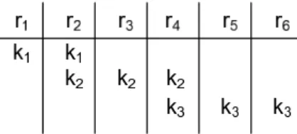
In a solution to the key distribution problem, one must be able to cover every posible subset of receivers because the privileged subset may be any of these subsets. For example, consider there are six receivers r1 through r6. Consider we
distribute three keys, k1, k2, k3 as follows. We give k1 to r1and r2; k2 to r2, r3 and
r4; k3 to r4, r5 and r6. (See Figure 2.1). With this distribution, one can cover the
subset {r1, r2} by encrypting the broadcast with only k1, or {r2, r3, r4, r5, r6} by
encrypting once with k2 and once with k3. However, one cannot cover the subset
{r3, r4}. In a valid key distribution, this situation should be prevented. Actually,
the rest is minimizing the number of keys per receiver called key storage, which is subject to the key distribution problem. At the moment the broadcast cover problem is encountered, keys have been already distributed to the receivers, and a particular broadcast, for which we know exactly which receivers are revoked and which are privileged, is ongoing. The problem is determining how many encryptions are needed and with which keys they should be done. Of course, we
CHAPTER 2. FREE RIDER PROBLEM AND SD SCHEME 9
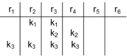
Figure 2.2: Example Subset Cover for Free Rider Demonstration
want minimize the number of encryptions, called transmission overhead, which is subject to the broadcast cover problem.
These two problems are strongly dependent when free riders are not allowed. We cannot improve one of them without affecting the other, because once we design a solution for the first problem, solution to the second problem becomes deterministic. But once free riders are allowed, transmission cost can be reduced without affecting the key storage. To demonstrate this idea, consider the following example. Let we have six receivers r1 through r6, and let k1 is given to r2 and
r3; k2 is given to r3 and r4; k3 is given to r1, r2, r3, and r4; and k4 is given to
r5 and r6 See Figure 2.2. Now suppose that we have three privileged users, r2,
r3, and r4. We can cover these receivers by using keys k1 and k2, and have a
transmission overhead of 2. However, if we allow 1 free rider, we can use it for r1 and use only k3 which leads us to a transmission overhead of 1. Note that we
placed the free rider not randomly but cleverly. With a random placement, the probability of success would be 1/3. Here, we see that assigning the only free rider to r1 is obviously the optimum solution. However, when we have lots of
receivers and lots of free riders allowed, it is not an easy task any more. Note that to deal with the problem of broadcast cover with free riders we must find a solution to the key distribution problem first and fix it. In this thesis, we choose the key distribution of SD scheme, because it has a decent key storage cost and it has the best transmission overhead cost found so far. We will explain the SD scheme in detail in the next section, however, to see the progress in this topic and appreciate SD, we must first consider some older ideas. We first explain three extremely simple broadcast encryption schemes.
• Key per receiver: Give every receiver a unique key. To make a broadcast, encrypt with only the keys of the privileged users. This scheme has a
CHAPTER 2. FREE RIDER PROBLEM AND SD SCHEME 10
perfect solution to the key distribution problem with only 1 key storage per receiver, however, the center has to make lots of encryptions for each broadcast. Assuming there may be a million privileged users in a broadcast for a cable TV program, it has an awful transmission overhead.
• Key per subset: Give all possible subsets of receivers a unique key, and upon a broadcast need, just use the key of the subset that contains only the privileged users. This scheme has a perfect transmission overhead with only 1 encryption, however, every receiver have to store 2N −1 keys, which is
sim-ply impossible even with a receiver population of hundreds, not thousands or millions.
• Broadcast to all: Give the same key to every receiver and encrypt with it in every broadcast. This scheme has an optimum key storage and transmis-sion overhead complexity, however, the revoked users are always free riders, which is contrary to the essence of broadcast encryption. Because even if we want to allow a number of free riders to reduce transmission cost, we have to have a bound on the number of free riders.
To supply the demand for a broadcast encryption scheme with the capability of extracting any possible subsets and requiring decent amount of key storage at the receivers, the tree structure of the LKH scheme was appropriate. In this design, key distribution is done as follows. First consider a binary tree whose leaves are associated with a different receiver. Now suppose we associate every node with a unique key. Then, for every node x, we give the key associated with x to all receivers associated with a leaf which is a descendent of x. If we look from the other way around, to each receiver, we give the keys of the nodes on the path from the root to the leaf associated with that receiver. Since the length of this path is log N for a balanced tree, key storage complexity turns out to be O(log N ), which is quite good, because even with a million receivers we have approximately twenty keys per receiver.
CHAPTER 2. FREE RIDER PROBLEM AND SD SCHEME 11
2.2.1
Tree Scheme and f-Cover Algorithm
Now we explain Tree Scheme of [4], which introduced the idea of allowing free rid-ers in broadcast encryption. The key distribution of the scheme is same as LKH, explained above. In the broadcast cover algorithm, the center first determines a constant, which the authors call redundancy, denoted by f , indicating the allowed ratio between the number of receivers that will be able to decrypt and the number of privileged users. For a node, if the ratio of receivers who can decrypt to the privileged receivers under it is less than f , they call it an f-redundant node. The f-Cover algorithm starts from the root and traverses the tree in a depth-first or breadth-first order, and checks every node whether it is f-redundant or not. When it encounters with an f-redundant node, it marks that node and does not traverse its descendants any more. At the end, the keys of the marked nodes are the ones that will be used. Thus, transmission overhead is the number of marked nodes. Note that the assignment of the free riders is not optimal in this method. Optimal solution to this problem is given in [19].
2.2.2
The Complete Subtree Scheme
After [4], research on the free rider problem slowed down for a while. The reason was that researchers focused on the special case where there are a small number of revoked users and the real aim is to revoke the illegitimate users. Obviously, free rider approach was not reasonable in this case. Therefore, [7] proposed the complete subtree scheme, which is almost same as the special case of the tree scheme where redundancy is 0. The result of the CS scheme is the same as the tree scheme with no redundancy but its processing method is different. CS scheme processes as follows.
First Steiner tree induced by the leaves associated with the revoked users, ST (R) is found. Then traversing ST (R), every node that hang off ST (R) is marked. At the end, keys of the marked nodes are used to encrypt the broadcast.
CHAPTER 2. FREE RIDER PROBLEM AND SD SCHEME 12
Note that the transmission cost can be approximated to O(r log N ) by con-sidering there are r receivers therefore r paths between the corresponding leaves and the root, and these paths are of length log N . However, this is only an upper bound. Considering also the intersections of these paths, they proved that the transmission cost of the CS scheme is O(r log N/r).
Complete subtree scheme was the last point in broadcast encryption research before SD scheme. However it did not consider the case where free riders are allowed. The solution to this case is given recently by [19] using a dynamic programming approach.
2.2.3
CS with Optimal Free Rider Assignment
Recently, Ramzan and Woodruff [19] proposed an algorithm which assigns free riders optimally in CS scheme. The algorithm does the following.
First it finds the Steiner tree ST (R) of revoked users. Then traverses this tree in postorder by recording the best subsolutions for each node and for each number of free riders allowed. In each calculation of a optimal solution, it uses the optimal subsolutions of the descendant nodes, which was previously solved and recorded. Using this dynamic programming approach, it finds the optimal solution to the problem in O(rf ) time.
The authors said that this approach may be applicable to other subset cover schemes like SD, however, they did not give a solution for SD. The problem we attack in this thesis is to find a way to optimally assign free riders for SD scheme.
2.3
The Subset Difference Scheme
We now explain the SD scheme, which is another subset cover scheme, in detail. Note that for a broadcast encryption scheme in subset cover framework, the more the subsets, the easier to cover a privileged receiver set with more accuracy. Using
CHAPTER 2. FREE RIDER PROBLEM AND SD SCHEME 13
this idea, Naor et al. [7] proposed the SD scheme which increases the number of subsets by simply assigning more keys to each receiver, but in a clever way.
Key Distribution. As in any subset cover broadcast encryption scheme, a collection of subsets is defined first.
S = {Si,j|xj is a descendant of xi}
where
Si,j = {x|x is a leaf and x is a descendant of xi and x is not a descendant of xj}
Note that the subset Si,j contains the receivers whose associated leaves are
descendants of xi but not descendants of xj. Intuitively, subsets of SD scheme are
exactly the differences of those of CS scheme. Note that a subset of CS scheme rooted by node x, can be found in the subsets of SD which is Sparent(x),sibling(x).
However, since the root has no parents, full tree cannot be found in the SD subsets, therefore a special subset which is the full tree is added. Each subset Si,j
is associated with a key Ki,j. The key distribution in [7] is performed in a clever
way for reducing key storage to O(log2N ). A user is not given all of the keys of the subsets which contains it, but given some of them such that it can calculate all of them. This key assignment method has nothing to do with the problem of this thesis, so we skip the details.
Covering Algorithm. For a revoked user set R, First the Steiner tree ST (R) is found. Then a temporary tree T is maintained and initialized to ST (R). Then, the following steps are run until there is only one node in T .
• If there is only one leaf y, add Sroot,yto the cover, and remove all descendants
of the root.
• Else, find two leaves y and z whose lowest-common-ancestor x has no other leaves in T . W.l.o.g. suppose y is on the left of z.
CHAPTER 2. FREE RIDER PROBLEM AND SD SCHEME 14
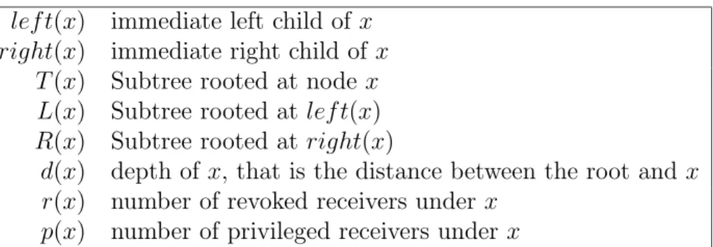
lef t(x) immediate left child of x right(x) immediate right child of x
T (x) Subtree rooted at node x L(x) Subtree rooted at lef t(x) R(x) Subtree rooted at right(x)
d(x) depth of x, that is the distance between the root and x r(x) number of revoked receivers under x
p(x) number of privileged receivers under x Table 2.1: Preliminary Notation – If right(x) 6= z, add Sright(x),z to the cover.
– Remove all descendants of x from T and make x a leaf node.
Decryption Step. Same as all other broadcast encryption schemes in subset cover framework.
With the covering algorithm above, it is guaranteed that the cover size is at most 2r − 1. For the formal proof, see [7].
2.4
Definitions
In this section we give the necessary definitions for the algorithms in chap-ters 3 and 4. First, we recall the notations. We denote the set of all users by U , with |U | = N , the set of revoked users for a particular broadcast by R, with |R| = r, the set of privileges users by P , with |P | = p, and the set of free riders by F , with |F | = f .
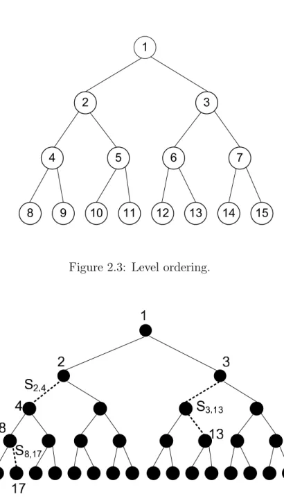
Throughout the thesis, for a binary tree, we use the preliminary notation in Table 2.1. We give numbers to the nodes in level order, that is we give 1 to the root, and recursively for any node x with number i, we give 2i to lef t(x) and 2i + 1 to right(x). See Figure 2.3. We denote a node by xi if it is numbered with
CHAPTER 2. FREE RIDER PROBLEM AND SD SCHEME 15
Figure 2.3: Level ordering.
CHAPTER 2. FREE RIDER PROBLEM AND SD SCHEME 16
Definition 1 (SD configuration) We call the combination of a tree T and a collection C of Si,j subsets on it an SD configuration. See Figure 2.4 This
con-figuration can be a solution to an SD problem or not. But every SD solution is an SD configuration. We also use this term for subtrees specifically as the SD configuration of T (x).
Definition 2 (i-point, j-point) In a particular SD configuration, let Si,j be the
subset for covering under node xi but not node xj. Then, we call xi an i-point
and xj a j-point.
Definition 3 (SD solution) We call an SD configuration an SD solution if it constitutes a valid solution for the current SD problem. i.e. If the union of the Si,j subsets in the collection C of the configuration covers the privileged users and
covers no more than allowed number of free riders.
Definition 4 (Cost) Cost of an SD configuration or an SD solution is defined as the number of Si,j subsets it contains. We also refer to the cost of a SD
configuration of T (x) with ‘the cost under x’.
Note that in exact schemes cost is a function of only revoked leaf positions, but when we have free riders, number of free riders available will also affect the cost. Therefore, minimum cost of an SD configuration becomes a function of revoked user positions and number of free riders available for x. We have slightly different definitions for the optimal solution and its cost, so we postpone their definitions to the related chapters.
For running time efficiency concerns, our algorithms will run only on a special set of nodes, the meeting points.
Definition 5 (Meeting Point) We call a node x a meeting point if both L(x) and R(x) contain some revoked users or if it is a leaf node. We call the former type inner meeting point.
CHAPTER 2. FREE RIDER PROBLEM AND SD SCHEME 17
Since for any inner meeting point x there will be some meeting points in both L(x) and R(x). We denote the highest such meeting points in the left and right subtrees as mpl(x) and mpr(x), respectively.
Chapter 3
Greedy Algorithms
In this chapter we present three greedy algorithms which attacks the problem of efficiently assigning a designated number of free riders to a broadcast encryption instance to reduce transmission overhead.
3.1
Top-Down Algorithm
The aim in this algorithm is to cover the privileged users with as few as possible subsets. Therefore, it is better to have our Si,j subsets such that i is as high
as possible. So, we trace the tree from the top to the bottom by checking each node, assuming it is an i-point, whether it satisfies the redundancy bound with some appropriate j-point or not. Now we give the algorithm and then explain the details. Top-Down-Assign(T , R, f ) f ratio ← (f + p)/p Find-Best-Exclusion-Point(root) Top-Down-Cover(root) 18
CHAPTER 3. GREEDY ALGORITHMS 19 Find-Best-Exclusion-Point(x) if r(x) > 0 then if x is a leaf or p(x) = 0 then bep(x) ← x return x else y ← Find-Best-Exclusion-Point(lef t(x)) z ← Find-Best-Exclusion-Point(right(x)) if z = null or r(y) > r(z) then bep(x) ← y return y else bep(x) ← z return z
else return null
Top-Down-Cover(x)
if (p(x) + r(x) − p(bep(x)) − r(bep(x)))/(p(x) − p(bep(x))) ≤ f ratio then C ← C ∪ {Sx,bep(x)}
else if r(x) = 0
then C ← C ∪ {Sparent(x),sibling(x)}
else Top-Down-Cover(lef t(x))
Top-Down-Cover(right(x))
The algorithm uses a greedy approach and basically does the following: It first finds the ratio
f ratio = (f + p)/p
which is called the redundancy of the broadcast.
First step of the algorithm finds a best exclusion point for every node in the tree. Best exclusion point of node x is the descendant of x which has the most number of revoked users and has no privileged users under it. Best exclusion
CHAPTER 3. GREEDY ALGORITHMS 20
point is denoted by bep(x). The reason why we choose this node is clear: The minimum redundancy is achieved with such a j-point because we exclude revoked positions as much as possible. This step is simply done recursively in a depth-first manner in O(N ) time.
The Top-Down-Cover procedure traces the tree in depth-first order by checking each node x whether Sx,bep(x) satisfies the redundancy bound. If it does,
the algorithm adds it to the cover and no longer traces its descendants. Then it checks whether all of its receivers are privileged or not. If this is true, it adds Sparent(x),sibling(x) to the cover. Otherwise, it recursively traces its children.
Eventually, the algorithm finds a cover which satisfies the redundancy bound. This can be proved easily by noting that all Si,j subsets satisfies the redundancy
bound, f ratio. Therefore, the union of these sets should give a redundancy lower than f ratio as well.
Note that this algorithm requires the redundancy bound to hold at each Si,j
taken. However, in an optimal solution it may be the case that a few subsets have a slightly higher redundancy but all other subsets has lower redundancies so that the overall redundancy satisfies the bound.Another restriction is that it does not permit any subsets in the cover to be one under another unless the higher one has no redundancy, i.e. if Si,j is covered, we cannot add another
subset Si0,j0 where i0 is a descendant of j unless Si,j covers only original privileged
users. However, an optimal solution may have such a configuration. Also note that some free rider quota may remain after this algorithm, which means there is still room for improvement. Next, we will see an algorithm which does not have these drawbacks.
3.2
Bottom-Up Algorithm
In this section, we will describe an algorithm which starts with an initial SD solution, and by making free rider assignments step by step, produces a better SD solution. In each step it assigns free riders to a node, i.e. to all revoked
CHAPTER 3. GREEDY ALGORITHMS 21
receivers under a node. The intuition behind the algorithm can be explained with a few observations concerning the assignment of free riders:
• Given an initial SD solution, the aim of the algorithm is to get rid of some Si,j subsets by saturating T (j). So, in an atomic free rider assignment
event we assign free riders to the j-point of a subset Si,j in the current
configuration and remove this subset. Removal of a subset may or may not reduce the cover size, i.e. transmission overhead.
• The algorithm starts with the exact SD cover and checks each subset Si,j
in it to see how much benefit can be obtained by removing it. Once it finds the most beneficial subset, it removes it by saturating T (j) with free riders. When a subset Si,j is removed from a cover, since T (xi) must be covered,
another subset, Sparent(i),sibling(i) should be added. See Figure 3.1.
Figure 3.1: Removal of Si,j leads to insertion of Sinew,jnew
• When we add a subset to the cover, we need to check whether it can be merged with another subset. This can only happen when i-point of a subset is the j-point of another.
Now we define the profit gained by removing a subset Si,j formally. Consider
an initial SD configuration C. When we remove a subset Si,j by saturating its
j-point, let the new configuration be C0. The difference Cost(C) − Cost(C0) is
CHAPTER 3. GREEDY ALGORITHMS 22
The profit that will be obtained by removing an Si,j subset by saturating T (j)
can be one of the three:
• 0: There will be no profit if the subset Sparent(i),sibling(i) cannot be merged
with any other subset. This happens when neither parent(i) is j-point of another subset nor sibling(i) is an i-point of another subset. See Figure 3.2
Figure 3.2: No profit
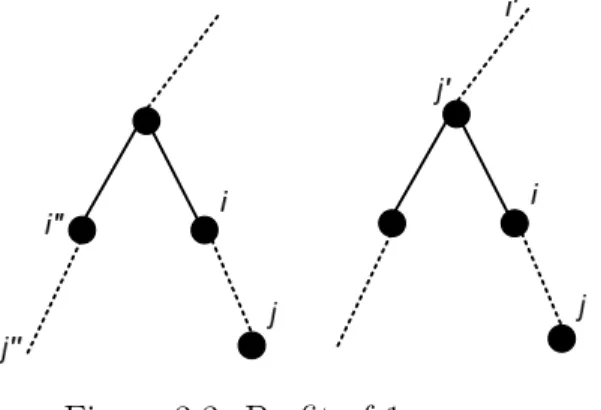
• 1: A profit of 1 will be gained when the subset Sparent(i),sibling(i) can only be
merged with one of Si0,parent(i) and Ssibling(i),j00. See Figure 3.3.
Figure 3.3: Profit of 1
• 2: As the best case, a profit of 2 will be gained when Sparent(i),sibling(i) can
be merged with both Si0,parent(i) and Ssibling(i),j00. See Figure 3.4
CHAPTER 3. GREEDY ALGORITHMS 23 Figure 3.4: Profit of 2 Bottom-Up-Assign(T , R, f ) S ← SD-Exact-Cover(T , R) SL ← Get-Sorted-Subset-List(S, f ) S ← Remove-Most-Profitable-Sets(S, SL, f )
Here, Get-Sorted-Subset-List algorithm produces a list SL of Si,j subsets,
where r(j) ≤ f , in descending order according to their advantage ratios, which is defined as:
ratioadv(Si,j) =
prof it(Si,j)
r(j) Remove-Most-Profitable-Sets(S, SL, f ) while SL 6= ∅ do Si,j ←Extract-First(SL) S ← S\{Si,j} Remove(SL, Si,j) if Jparent(i) = 1
then inew ← iptrparent(i)
S ← S\Sinew,parent(i)
Remove(SL, Sinew,parent(i)) else inew ← parent(i)
if Isibling(i) = 1
then jnew ← jptrsibling(i)
CHAPTER 3. GREEDY ALGORITHMS 24
Remove(SL, Ssibling(i),j
new)
else jnew ← sibling(i)
f ← f − r(j) Clear(SL, r(j)) Saturate(j) S ← S ∪ Sinew,jnew Insert(SL, Si new,jnew)
Remove-Most-Profitable-Sets(S, SL, f ) algorithm removes the Si,j sets
one by one starting from the most profitable one until the remaining number of free rider assignments is not enough.
First, it gets the most profitable subset Si,j with Extract-First procedure.
Then it removes it from the cover and the subset list SL. Before adding the subset Sinew,jnew, it first checks whether it can be merged with other subsets or
not. Since there are two possible such subsets, it checks them and removes them if they exist, and updates inew and jnew points if necessary. Then it decreases the
free rider quota f by r(j) and calls the Clear subroutine which clears the list SL from the Si,j subsets having r(j) > f . At this point, the procedure have to
correct r(x) for each node x above j. This will also yield some changes in the advantage ratios, possibly changing the order of some subsets in SL. This is done in the procedure Saturate. Finally it inserts the new subset Sinew,jnew.
Now we discuss the running time of this algorithm. Since the dominating procedure is Remove-Most-Profitable-Sets we can omit the running times first two procedures. Note that if r(j) ≤ f for all subsets. So, there can be subsets of f − 1 different r(j) values, namely 1 to f . Thus, in each step either f decreases by one or all subsets Si,j with a particular r(j) value is removed. Therefore
while loop makes at most O(f ) iterations. In each iteration, Remove, Insert, and Clear procedures has O(r), the Saturate procedure has O(log N log f ) complexity. Hence, the overall complexity turns out to be O(f r + f log N log f ). Bottom-Up algorithm has the obvious drawback of any greedy algorithm: It does the right thing locally, but this may not turn out to be the best thing globally.
CHAPTER 3. GREEDY ALGORITHMS 25
Especially when a large number of free riders are allowed, a worse performance should be expected from the this algorithm. On the other hand, it is slower than the Top-down algorithm of the previous section.
3.3
Hybrid Algorithm
So far, we have described two greedy algorithms with their respective advantages and disadvantages. Below, we describe an algorithm where we use the Top-down algorithm to get the initial subset collection for the Bottom-up algorithm instead of using the exact cover solution. This yields a result faster but a little worse transmission overhead compared to the original Bottom-up algorithm. Here is the algorithm:
Hybrid-Assign(T , R, f )
S ← Top-Down-Assign(T , R, f ) SL ← Get-Sorted-Subset-List(S, f )
S ← Remove-Most-Profitable-Sets(S, SL, f )
The algorithm first runs the Top-Down-Assign subroutine, then continues same as the Bottom-up algorithm. Forms the sorted subset list according to the averages and remove one by one at each step until spending all free rider quota.
Note that the running time of the algorithm is somewhere between that of the Top-down algorithm and the Bottom-up algorithm, because it basically runs the Top-down algorithm and then calls some other procedures, or looking from the other way around, it arrives at the second line of the Bottom-Up algorithm with a smaller f value yielding a much faster run for the last two lines.
In Chapter 5, we will compare the performance of this algorithm with the previous two.
Chapter 4
Optimal Free Rider Assignment
for the SD Scheme
In this chapter, we give two optimal free rider assignment algorithms for the SD scheme. Both algorithms are based on a dynamic programming approach. In fact, the algorithms are similar in essence but the difference is that the first algorithm is more intuitive but the second one is faster.
4.1
The Optimization Algorithms
We will describe an algorithm based on a dynamic programming approach in order to get the optimal SD solution for given a set of revoked users R, and a number of free riders f . We will run the algorithm on meeting points and calculate the cost, with all possible assignments of free riders, using the costs of the closest descendant meeting points from left and right. Now, as the first step of dynamic programming, we characterize the structure of an optimal solution.
Definition 6 (Cost(x,n)) We denote the cost of an SD configuration for T (x) by assigning n free riders, as Cost(x, n). We define this cost as the minimum possible number of Si,j subsets covering leaves in T (x).
CHAPTER 4. OPTIMAL FREE RIDER ASSIGNMENT FOR SD 27
Consider a node x, let y = mpl(x) and z = mpr(x). Suppose f free riders are available to assign under x. Then, if we assign f (y) of these free riders under y and f (z) of them under z, the overall cost of x becomes:
Cost(x, f (x)) = Cost(y, f (y)) + Cost(z, f (z)) + Ey+ Ez
Here, Ey and Ez denotes the possible costs on the paths x through y and z
respectively.
Hence, in an optimal solution the summation of the costs of these four factors should be minimized. We can come up with a recursive solution as follows.
Cost(x, f (x)) = min
0≤f (y) 0≤f (z) f(y)+f (z)=f (x)
{Cost(y, f (y)) + Cost(z, f (z)) + Ey+ Ez}, (4.1)
where y = mpl(x), z = mpr(x), and Ey and Ez are the possible extra costs
originating from the paths from x to y and z respectively. Each of the last two factors can bring at most one extra cost, and it depends on some other conditions. We will explain these conditions in next two sections.
4.1.1
The Basic Algorithm
In this section, we first give the essence of the algorithm, then explain the details of the dynamic programming formulation, and then we give the conditions that make Ey = 1 and Ez = 1.
In the recursive step of the algorithm, which was formulated in (4.1), we derive the cost for a node using the costs at the lower meeting points and the paths towards them. Apparently, any node may be assigned any number of free riders in an optimal solution, therefore we should calculate a cost for all nodes and for all possible number of free riders that can be assigned to them.
CHAPTER 4. OPTIMAL FREE RIDER ASSIGNMENT FOR SD 28
In the basic algorithm, with Cost(x, n), we denote the minimum number of Si,j
subsets under node x, by assigning exactly n free riders under node x. Note that the optimal solution to a problem with f free riders available, may be obtained by using less than f free riders. To visualize this, suppose a receiver setting, where all users are privileged except the ones under a particular node which is not the root. Without assigning free riders, we have a cost of 1. However, when we assign a free rider, the cost increases. So, we cannot guarantee that the more free riders we assign, the less the cost is. As a result, we have to try assigning from 0 to f free riders to the root.
We can now explain how to calculate Ey and Ez. Due to their symmetry,
w.l.o.g., we will only explain for Ey. It syntactically stands for “extra cost between
x and y”. Semantically, it is the cost possibly originating from the path through x to y. There are three possibilities.
• Either there is no need for an Si,j subset lying between x and y,
• or there must be an Si,j subset but it can be merged with the Si,j subset
right underneath y,
• or there must be an Si,j subset and it cannot be merged with another one.
Let us investigate when one would need an Si,j subset between x and y.
• r(y) > f (y). First, number of revoked users under y must be greater than f (y). Otherwise, that is if r(y) = f (y), we would not need any subsets because we have enough free riders to fully saturate and make all r(y) revoked users under y free riders. Then, we leave the covering of the users under y to a subset of higher levels. There will be a subset in the higher levels of the tree, whose i-point is an ancestor of y, but its j-point is not. Thus, to get a 1 for Ey, it must be the case that r(y) > f (y). This condition
is necessary but not sufficient.
• y /∈ I. Another necessity is that y is not an i-point. Because, even if there exists an Si,j subset between x and y, it would be merged with the subset
CHAPTER 4. OPTIMAL FREE RIDER ASSIGNMENT FOR SD 29
underneath y. So, it does not matter whether there will be a subset between x and y because it will cancel anyway and bring no cost. This condition is also necessary but not sufficient.
• Given the above two conditions are both true, at least one of the following conditions must also hold in order to guarantee Ey = 1.
– d(y) − d(x) ≥ 2. If there are some nodes between x and y, that is d(y) − d(x) ≥ 2, there will be an extra subset between x and y, which will make Ey = 1 certainly, because of two reasons. First, since
there are some nodes which are not meeting points, between x and y, one children of each of these nodes has privileged users under them, therefore there has to be an Si,j subset such that its i-point is above
these nodes. So, there are only two possibilities: x, and the left child of x. Second, since y has both privileged and remaining revoked users, there must be a j-point somewhere under y. But, since y is not an i-point, this j-point cannot be the j-point of x or lef t(x), one of which we have proved to be an i-point. Then the only possibility for the j-point is y. Thus, we end up with an Si,j subset, whose i-point is x
or lef t(x), and j-point is y. Therefore, in both cases, we will have an extra cost, that is Ey = 1.
– r(z) = f (z). Now, assume the condition above does not hold, meaning y is the immediate left child of x. Then only possibility for an Si,j
subset between x and y is the subset whose i-point is x and j-point is y. Note that this means the subtree of the right child of x is fully saturated. Therefore z must be fully saturated. Then we must have r(z) = f (z) to saturate z and get Ey = 1.
Thus, the first two conditions, together with either d(y) − d(x) ≥ 2 or r(z) = f (z) is sufficient to get an extra subset between x and y and make Ey = 1.
Throughout the algorithm, we keep the meeting points in an array called M P , for efficient implementation. M P is prepared by the Find-Meeting-Points
CHAPTER 4. OPTIMAL FREE RIDER ASSIGNMENT FOR SD 30
subroutine as follows. First, M P is initialized to leaves that are associated with the revoked users and mark all of them. Then we choose two marked meeting points mp1 and mp2 such that their lowest common ancestor mpc has no other
de-scendent marked meeting points. We add mpc to M P , mark it, and unmark mp1
and mp2. We progress until only one marked meeting point remains. Eventually,
we end up with a meeting point list in which a meeting point always comes before its ancestors. Therefore, when we trace this array in order, we always arrive at a meeting point after its descendants. We also know that first r are the leaves and the rest, r + 1 through 2r − 1 are the inner meeting points.
For any meeting point x and any possible number of free riders assigned to it, we also need to keep track of the optimal cost found for x, number of free riders assigned to left subtree of x, and a flag indicating whether x is an i-point or not in the optimal configuration. The arrays we use to hold this information are Cx,
Lx, and Ix, respectively. Free-Rider-Assign-Basic(T , R, f ) M P ← Find-Meeting-Points(R) for i ← 1 to r x ← M P [i] Cx ← [0, 0] Ix ← [0, 0] for i ← r + 1 to 2r − 1 x ← M P [i] y ← mpl(x) z ← mpr(x) for f (x) ← 0 to min(r(x), f ) Cx[f (x)] ← ∞
for f (y) ← max(f (x) − r(z), 0) to min(r(y), f (x)) f (z) = f (x) − f (y)
tempcost ← Cost(y, f (y)) + Cost(z, f (z)) + Ey,f(y)+ Ez,f(z)
if tempcost < Cx[f (x)] or
³
tempcost = Cx[f (x)] and (r(y) = f (y) or r(z) = f (z))
CHAPTER 4. OPTIMAL FREE RIDER ASSIGNMENT FOR SD 31 then Cx[f (x)] ← tempcost Lx[f (x)] ← f (y) if f (y) = r(y) or f (z) = r(z) then Ix[f (x)] = 1 else Ix[f (x)] = 0
/* Now calculating the optimal cost for the root */ result ← ∞
for f (root) ← 0 to f
rootcost ← CM P[2r−1][f (root)]
if depth(M P [2r − 1]) 6= 0 and IM P[2r−1][f (root)] 6= 1
then rootcost ← rootcost + 1 if rootcost < result
then result ← rootcost return result
where Ey,f(y)=
(
1 if r(y) > f (y) and y /∈ I and (d(y) − d(x) ≥ 2 or r(z) = f (z)) 0 otherwise
and similarly, Ez,f(z) =
(
1 if r(z) > f (z) and z /∈ I and (d(z) − d(x) ≥ 2 or r(y) = f (y)) 0 otherwise
First, the meeting points are found. This is a rather easy task, which can be performed very fast, starting from revoked users and run in a bottom-up fashion, as we mentioned earlier. Then, we fill C and I arrays of the leaves with zeros. This is trivial since there cannot be any subsets under a leaf and it cannot be an i-point. In the rest of the algorithm, we trace the meeting points in an bottom-up fashion, so that when we arrive any meeting point x, we have both solutions for mpl(x) and mpr(x). At each meeting point x, we find optimal solutions for all possible free rider count for x. For a particular number of free riders f (x) for x, we find all costs and corresponding I and L arrays with possible partitions of free riders assigned to x to its children. Among these, we take the one with
CHAPTER 4. OPTIMAL FREE RIDER ASSIGNMENT FOR SD 32
minimum cost. If there occurs a tie between two or more partitions, we prefer the one which makes x an i-point. This is very intuitive because when x is an i-point, there is a probability for it to be merged with the subset just above. Otherwise, it cannot be merged. Thus, making x an i-point is at least as good as not making so. Algorithm finally considers –for all possible number of free riders– the costs of the root meeting point together with the cost over it, since there can possibly be other nodes over the highest meeting point, which means it is not the root of the real tree. This can occur when all revoked users are grouped under a node which is not the root. In such a situation, we must add a cost of 1 for the Si,j
subset, whose i-point is the root of the real tree, and j-point is the root of the Steiner tree, unless the root meeting point is an i-point. The running time of the algorithm is O(rf2) in the worst case, yet this is a loose bound.
4.1.2
Improved Algorithm
In this section, we present a slightly improved algorithm. Basically it has the same essence as the basic algorithm but by changing the definition of Cost(x, n) we save the computation for finding actually how many free riders leads to the minimum cost which is done at the root meeting point.
In this algorithm, with Cost(x, n), we denote the minimum cost under node x, by assigning at most n free riders under node x.
The basic algorithm and this one differ in two points. First, we do not calculate the cost of the root meeting point with free rider counts less than f . So, instead of taking minimum among all free rider counts, we take Cost(root, f ) as the result directly. Second, Ey and Ez are defined differently in this algorithm. In fact,
we introduce a few more cases in their definitions. We will now explain these differences in detail.
The first difference is more intuitive and clear. With the new Cost(x, n) definition, we handle all free rider counts equal to and less than f at once. To make it even more clear, we do not need to calculate Cost(x, n0) where n0 < f
CHAPTER 4. OPTIMAL FREE RIDER ASSIGNMENT FOR SD 33
because we are sure that there are f free riders available for the root. So, there is no need to bound the number of free riders to any number less than f and calculate a cost for the root meeting point.
The difference we made in the definition of Cost(x, n) does not change the structure of an optimal sub-solution at the high level description. We still have the recursive formula (4.1). However, we need to change the definitions of the extra costs Ey and Ez.
We now explain how to calculate Ey and Ez. As we did in the basic algorithm,
due to their symmetry, w.l.o.g., we will only explain for Ey. We have the same
three possibilities as in the basic algorithm.
• Either there is no need for an Si,j subset in this path
• or there must be an Si,j subset but it can be merged with the i-j pair just
below it.
• or there must be an Si,j subset and it cannot be merged with another one
Let us now investigate when one would need a subset between x and y.
• First, number of revoked users under y must be greater than f (y). Oth-erwise, r(y) = f (y), and this means we fully saturate and make all r(y) revoked users under y free riders. Then, we leave the covering of the users under y to a subset of higher levels. Thus, to get a 1 for Ey, it must be the
case that r(y) > f (y). Notice this condition is same as the first condition in the basic algorithm. Again, it is necessary but not sufficient.
• Second, y must not an i-point in this Ey definition as well. Because, again
similar to the Ey definition of the previous algorithm, even if there exists a
subset between x and y, it would be merged with the subset underneath y. This condition is also necessary but not sufficient.
• Given the above two conditions are both true, at least one of the following conditions must also hold in order to guarantee Ey = 1.
CHAPTER 4. OPTIMAL FREE RIDER ASSIGNMENT FOR SD 34
– There must be some nodes between x and y. Then, there will be an ex-tra subset between x and y, which will make Ey = 1 certainly, because
of two reasons which are exactly same as the ones in Ey definition of
the previous algorithm.
– Now, assume the condition above does not hold, meaning y is the im-mediate left child of x. Then only possibility for a subset Si,j between
x and y is the subset whose i-point is x and j-point is y. Note that this means the subtree of the right child of x is fully saturated. Therefore, z must be fully saturated. Then there are two necessary conditions which are sufficient together to saturate z and get Ey = 1.
∗ First, we must have enough free riders to be able to saturate z, that is r(z) ≤ f (z). This condition is obviously necessary but not sufficient alone. We need the following condition as well.
∗ Note that when we have an Si,j subset with x as the i-point and
y as the j-point, we fully saturate the subtree rooted at the right child of x, which is either z or the highest node between x and z. However, in order for this subset to make sense, there must be some privileged users under this saturated subtree. That is, it should not be the case that this subtree is fully revoked and we add a subset with a possible extra cost, just because we are able to. Therefore, it must be the case that p(z) > 0 or d(z)−d(x) ≥ 2. If these two conditions both hold, then one should fully saturate z. Otherwise it is not advantageous.
Thus, the first two conditions, together with either d(y) − d(x) ≥ 2 or ³
r(z) ≤ f (z) and (p(z) > 0 or d(z) − d(x) ≥ 2)´. is sufficient to get an extra cost between x and y.
We still have the same data structures for a node x: Cx, Ix, and Lx. This time,
ith element of C
x holds the optimal cost found for T (x) by assigning at most i
free riders under x. Then, Ix and Lx is defined correspondingly. M P array is
CHAPTER 4. OPTIMAL FREE RIDER ASSIGNMENT FOR SD 35 Free-Rider-Assign-Improved (T , R, f ) M P ← Find-Meeting-Points(R) for i ← 1 to r x ← M P [i] Cx ← [0, 0] Ix ← [0, 0] for i ← r + 1 to 2r − 1 x ← M P [i] y ← mpl(x) z ← mpr(x) for f (x) ← 0 to min(r(x), f ) if i = 2r − 1 then f (x) ← min(r(x), f ) Cx[f (x)] ← ∞
for f (y) ← max(f (x) − r(z), 0) to min(r(y), f (x)) f (z) = f (x) − f (y)
tempcost ← Cost(y, f (y)) + Cost(z, f (z)) + Ey,f(y)+ Ez,f(z)
if tempcost < Cx[f (x)] or
³
tempcost = Cx[f (x)] and (r(y) = f (y) or r(z) = f (z))
´ then Cx[f (x)] ← tempcost Lx[f (x)] ← f (y) if f (y) = r(y) or f (z) = r(z) then Ix[f (x)] = 1 else Ix[f (x)] = 0 result ← CM P[2r−1][f ] if depth(M P [2r − 1]) 6= 0 and IM P[2r−1][f ] 6= 1
then result ← result + 1 return result
CHAPTER 4. OPTIMAL FREE RIDER ASSIGNMENT FOR SD 36 where Ey,f(y)=
1 if r(y) > f (y) and y /∈ I and à d(y)-d(x) ≥ 2 or ³r(z) ≤ f (z) and (p(z) > 0 or d(z) − d(x) ≥ 2)´ ! 0 otherwise and similarly, Ez,f(z) = 1 if r(z) > f (z) and z /∈ I and Ã
d(z)-d(x) ≥ 2 or ³r(y) ≤ f (y) and (p(y) > 0 or d(y) − d(x) ≥ 2)´ !
0 otherwise
In this version of the algorithm, the improvement is on the number of cost calculations. The difference comes from the root node. Although the theoret-ical bound remains same, the actual cost decreases. This improvement can be observed in the next section, which contains our experimental results.
Chapter 5
Experimental Results
In this chapter, the experiments conducted to compare the performances of the algorithms explained in chapters 3 and 4, are presented. To see the advantage of the free riders, the algorithms are also compared with the original SD scheme of [7], which is the best scheme in terms of transmission cost discovered so far in no-free-rider case.
The organization of the chapter is as follows: We first describe the evaluation parameters. Then, we briefly explain the implementation. Finally, we give the experimental results which compare the performances of our algorithms as well as the original SD scheme, in terms of transmission overhead with different values of the input parameters.
5.1
Evaluation Parameters
As we explained in detail in Chapter 2, we fix the key distribution to the one described in original SD scheme, and focus on the transmission overhead. There-fore, the primary evaluation parameter in this thesis is the transmission overhead, which is a function of the following four variables:
CHAPTER 5. EXPERIMENTAL RESULTS 38
• N , number of all receivers. • R, the set of revoked receivers. • r, the number of revoked receivers.
• f , the number of free riders allowed. i.e. free rider quota.
Another performance measure is, like almost all computer-related work, the running time complexities of the algorithms.
5.2
Implementation Issues
Consider the four factors that affect the transmission overhead we mentioned above. Throughout the experiments, we choose and fix a reasonable number N = 1024 for the number of receivers, and we take 100 runs for every number of privileged users possible, i.e. from 1 to 1024. We assume that the free rider quota is directly proportional to the number of privileged users. So use the f ratio definition of :
f ratio = (f + p)/p
Finally, we take the average transmission cost for a particular number of privileged users and corresponding free rider quota. We run this experiment for different values of f ratio, namely 2/1, 4/3, 8/7, 8/5, 16/15, 16/13. Thus we observe the changes in the performances of the algorithms when a larger free rider quota is available. We show the results on one graph per one f ratio value.
We also consider the execution times of the experiments explained above. We are particularly interested in the comparison of the two optimal algorithms and we want to see to what extent the greedy algorithms are close to them in terms of computation time.
CHAPTER 5. EXPERIMENTAL RESULTS 39
5.3
Experiments
In this section, we present the results of the experiments with appropriate graphs and tables and discuss them.
5.3.1
Transmission Overhead Experiments
The following graphs shows the transmission costs of the algorithms with respect to the target privileged user set size p and the corresponding free rider quota f , which is calculated as:
f = p(f ratio − 1)
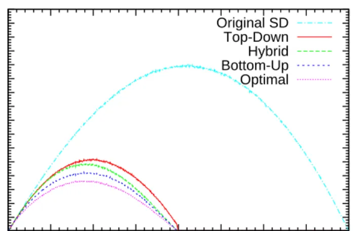
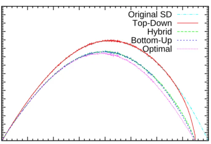
A different graph is presented for each f ratio value in Figures 5.1, 5.2, 5.3, 5.4, 5.5, and 5.6. 25 50 75 100 125 150 175 200 225 250 275 300 325 350 375 400 0 128 256 384 512 640 768 896 1024
Number of Transmissions
Target Size
f = 2.0 Original SD Top-Down Hybrid Bottom-Up OptimalFigure 5.1: Transmission costs of our algorithms with f = 2.0.
First of all note that as the free rider quota decreases, all of the algorithms converge to the original SD scheme as we expected. Another point to observe is that the transmission costs of the algorithms with free riders become 1 when
CHAPTER 5. EXPERIMENTAL RESULTS 40 25 50 75 100 125 150 175 200 225 250 275 300 325 350 375 400 0 128 256 384 512 640 768 896 1024
Number of Transmissions
Target Size
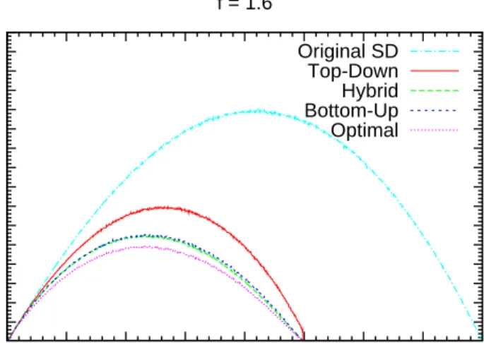
f = 1.6 Original SD Top-Down Hybrid Bottom-Up OptimalFigure 5.2: Transmission costs of our algorithms with f = 1.6.
25 50 75 100 125 150 175 200 225 250 275 300 325 350 375 400 0 128 256 384 512 640 768 896 1024
Number of Transmissions
Target Size
f = 1.34 Original SD Top-Down Hybrid Bottom-Up OptimalCHAPTER 5. EXPERIMENTAL RESULTS 41 25 50 75 100 125 150 175 200 225 250 275 300 325 350 375 400 0 128 256 384 512 640 768 896 1024
Number of Transmissions
Target Size
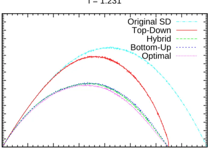
f = 1.231 Original SD Top-Down Hybrid Bottom-Up OptimalFigure 5.4: Transmission costs of our algorithms with f = 1.231.
25 50 75 100 125 150 175 200 225 250 275 300 325 350 375 400 0 128 256 384 512 640 768 896 1024
Number of Transmissions
Target Size
f = 1.143 Original SD Top-Down Hybrid Bottom-Up OptimalCHAPTER 5. EXPERIMENTAL RESULTS 42 25 50 75 100 125 150 175 200 225 250 275 300 325 350 375 400 0 128 256 384 512 640 768 896 1024
Number of Transmissions
Target Size
f = 1.067 Original SD Top-Down Hybrid Bottom-Up OptimalFigure 5.6: Transmission costs of our algorithms with f = 1.067.
N/p ≥ f ratio
because that means r ≤ f and one can saturate all receivers with the free rider quota available and make a single broadcast to everyone.
As the free rider quota decreases, the performance of the Top-Down algorithm gets worse faster than the other algorithms. This can be explained by the fol-lowing strong restriction of the Top-Down algorithm: It operates with the free rider ratio instead of the free rider count, and requires that this ratio holds in every subtree. Therefore, for example, when f = 1.067 = 16/15, the Top-down algorithm even has no chance in subtrees having less than 16 receivers, because in an Si,j subset in such a subtree, there can be at most 15 receivers, therefore
the only ratio smaller than 16/15 is 1, which leads to an exact cover which has no free riders. Hence, Top-down algorithm tends to operate in the higher levels of the tree and once it arrives at the lower levels that it cannot make improvements, a portion of the free rider quota remains and cannot be used. Actually this is one of the reasons why we devised the Hybrid algorithm.
CHAPTER 5. EXPERIMENTAL RESULTS 43
The Bottom-up algorithm and the Hybrid algorithm has close performances for lower free rider quota. Actually, the only significant difference between the performances of these algorithms is observed in the case where f = 2.0. Note that this case is also the one where the Top-down algorithm works best. There is a strong relation between these two observations: Since the the Hybrid al-gorithm is actually the successive runs of Top-down and Bottom-up alal-gorithms, when f = 2.0 the Top-down algorithm spends the free rider quota much more and leaves less free riders for the Bottom-up algorithm, therefore the Bottom-up algo-rithm cannot reduce the transmission cost much. However, when the Bottom-up algorithm works alone, it uses the portion of the free rider quota used by the Top-down algorithm within the Hybrid algorithm more effectively and gets a better performance compared to the Hybrid algorithm.
Note that the Bottom-up and Hybrid algorithms has a transmission cost pretty close to that of the optimal algorithms. The reason is that the drawbacks of the Bottom up algorithm is seen in very extreme cases. The advantage of the optimal algorithms compared to the Bottom-up algorithm is that they handle the situations where making a revoked user free rider does not have an advantage immediately but it leads to a better configuration afterwards.
5.3.2
Running Time Comparisons
In this section we compare the running times of: • The two optimal algorithms
• The greedy algorithms with each other
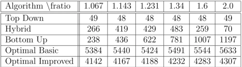
Table 5.1 shows the execution times of different algorithms with different free rider ratios. For each entry, the algorithms are run 100 times with each possible number of privileged users from 1 to 1024.
The results on Table 5.1 show that the greedy algorithms, especially the Top-down algorithm, run much more faster than the optimal algorithms, as expected.