Mars: A tool-based modeling, animation, and parallel rendering system

(1)

MARS" a tool-based

modeling, animation,

and parallel rendering

system

Murat Aktlhano lu, Biilent 0zgiig,

Cevdet Aykanat

Department of Computer Engineering and Information Science,

Bilkent University,

06533 Bilkent, Ankara, Turkey

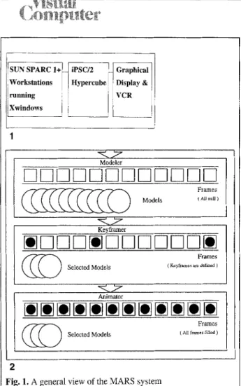
This paper describes a system for modeling, animating, previewing and rendering articulated objects. The system has a modeler of objects that consists of joints and segments. The animator interactively positions the articulated object in its stick, control vertex, or rectangular prism representation and previews the motion in real time. Then the data representing the motion and the models is sent to a multicomputer [iPSC/2 Hypercube (Intel)]. The frames are rendered in parallel, exploiting the coherence between successive frames, thus cutting down the rendering time significantly. Our main aim is to make a detailed study on rendering of a sequence of 3D scenes. The results show that due to an inherent correlation between the 3D scenes, an efficient rendering can be achieved.

Key words: Parallel r e n d e r i n g - - M u l t i - computer architectures-- parallel z-buffer a l g o r i t h m - - Keyframe a n i m a t i o n - - i n - between coherence.

Correspondence to: B. Ozgiiq

1 Introduction

The modeling, animation, and rendering system (MARS) is an ongoing study to provide a frame- work or environment for developing high-quality and cost-effective computer-generated anima- tions. The animator is presented with an interactive, flexible, powerful, and fast system. There have been several goals in designing MARS. First, the system is not intended for a specific application. It is a multipurpose animation gener- ator. Second, MARS tools were designed so that any of them can easily be replaced. New tools can be added to the system without disturbing the integrity of the environment. Third, MARS was designed so that it makes the most of the current resources in the development environment (Fig. 1).

The process of generating a computer animation by MARS can be broken down into three phases (Fig. 2): modeling, animation, and rendering. In the modeling phase, the modeler creates a 3D model of the scene and its components. In the animation phase, the animator describes how the model will change its place and orientation over time, generates the key-frames, and subsequently, using a simplified model of the object, views the motion described in real time. The most important tool of the system is the renderer. In the rendering phase, the renderer running on the iPSC/2 multicomputer currently with 32 processors, takes the model and animation data and, for each frame in the sequence, generates a 2D image with the specified shading algorithm and camera position.

2 Overview

In MARS, an animator can use graphical primitives or B-spline surfaces. The models can have any number of joints, thus any general object can be modeled. By transforming various segments of a model, many different versions can be created. The animator can switch among the many avail- able models by clicking them, and orient the current model by selecting an axis, an angle, and a joint from a menu (Heller 1990; Ozgii 9 1988). The rendering process, which is the most expensive phase of the three, is done by a multicomputer. The patches are rendered on 32 processors simultaneously. One of the most

(2)

SUN SPARC 1+~ Workstations ,[ running :[ [ Xwindows [ _ _ iPSC/2 IN Graphical Hypercube ~ Display &

l

VCR

Modeler

D N @ N 8 9

Frames Models ~ All nuR )

Keyframer

[] D D D

[] I--1D I--11--11--1161

~ ) Frames

Selected Models ( Keyfraxnes are detined )

Animator

Frames Selected Models ( Au f ~ , ~ f~Ued )

2

Fig. 1. A general view of the MARS system

Fig. 2. The process of generating a computer animation

important concepts in rendering is the distribution of the load among the processors, i.e., load- balance. This is achieved by a hybrid subdivision scheme that uses both object-space and image- space concepts. Moreover, the rendering is done even more efficiently by exploiting the temporal coherence that exists between the frames of the animation. Thus, the rendering time is shorter than that of the traditional straight-ahead ren- derers that work on uniprocessor machines and do not use the principle of coherence.

3 MARS modeler

The problem of presenting a 3D definition to the computer has been well researched in the past. There have been m a n y approaches and studies on

modeling in three dimensions (Cachola and Schrack 1986; Ferin 1990; Grosso et al. 1989; M a h m u d and Ozgii~, 1990, 1991; Ostby et al. 1990). The MARS modeler treats a model as a composition of a library of predefined or ready- to-use graphical primitives. The model consists of joints and their base segments, and the modeler connects these base segments with one another as specified in the joint definitions.

3.1 Joints

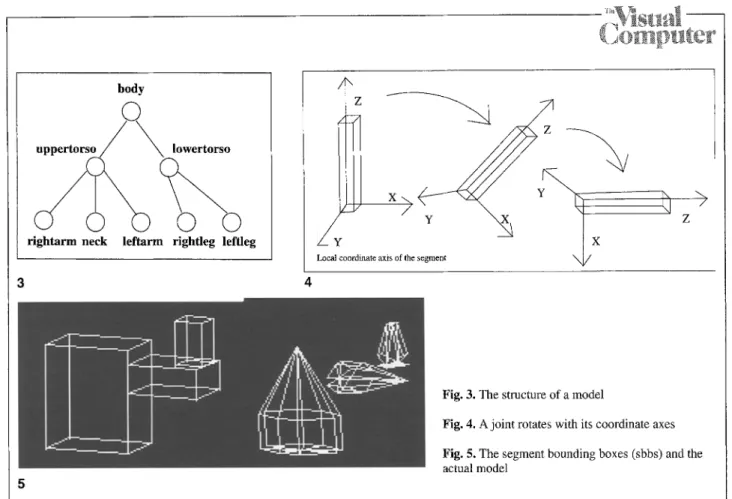
The joints form an n-ary tree structure (Fig. 3), i.e., the number of child joints of a given joint is not limited. Each joint has a parent joint and n chil- dren. Two vectors are used to define the X and Y axes of the joint. The Z-axis is the vector prod- uct of X and Y axes of that joint. A joint can be rotated about each of the X, Y, and Z axes, thus it has up to three degrees of freedom. With this method, simple joints, such as fingers (hinge joints) and complex joints, such as shoulders (ball-and-socket) can be simulated. Also, each joint has its own coordinate axis, contained in the definition of the model. Most of the time, the Z-axis is along the direction of the segment as a convention, but this can be modified to suit the needs of the animator. As a joint is rotated along its coordinate axes, the axes are also rotated, so it does not matter what the orientation of the joint with respect to the world coordinate axes is. The local coordinate axes are always aligned in the same way with respect to the segment (Fig. 4).

3.2 Segments

Each joint has a base segment that is defined with respect to its local coordinate axis. The segments of a MARS model are defined as B6zier surfaces (Ferin 1990; Rogers 1989, 1990; Watt 1989), but instead of directly giving a set of B6zier control points f o r each segment, the user first defines the segment bounding box

(sbb)

of the segment, which is simply the rectangular prism that bounds the segment itself, and then a set of B6zier control points. In fact, each base segment is defined in a unit cube, i.e., it is a set of normalized control points and their bounding box is a unit cube. Eventually this normalized segment definition is

(3)

omp er

body

uppertorso/Q~ lowertorso

LZo

r i g h t a r m neck leftarm rightleg

leftleg

3 4

\

Local coordinate axis of the segment

Z

Fig. 3. The structure of a model

Fig. 4. A joint rotates with its coordinate axes

Fig. 5. The segment bounding boxes (sbbs) and the actual model

scaled with respect to the defined sbb. If no sbb is defined, a unit cube is assumed (Fig. 5). As each segment's sbb is defined, we use this simpler rep- resentation in the positioning and previewing phases. This speeds u]~ the respective processes. For each segment of a model, a transformation matrix is kept for each frame. This matrix is generated from the local and the world coordinate axes and the joint positions. It is updated at every frame, should the segment change its place or orientation (Tokad 1990).

4 Animation

The MARS animator animates the 3D articulated rigid models using the parametric keyframe interpolation method, though there are many other methods in the literature (Badler 1986; Badler and Manoochehri 1986, 1987; Getto and Breen 1990; Hewitt et al. 1986; Jackson and Morris 1988; Magnenat-Thalmann and Thalmann 1985; Ostby et al. 1990; Shoemaker 1985; Wyvill et al. 1991).

4. 1 Interpolation strategy

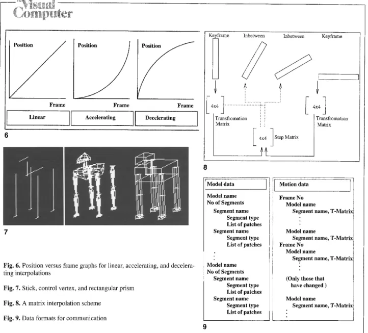
Inbetween frames are frequently linearly interpolated, resulting in temporal discontinuities and movements that only approximate actual trajec- tories and deform the animation (Badler 1987; Blinn 1987; Girard 1987). The MARS animator can interpolate the key frames by linear, acceler- ation, or deceleration methods. The position-versus-frame graphs are shown in Fig. 6. While the motion is being edited, simple representation techniques are used (Fig. 7). The matrix operations during the interpolations are shown in Fig. 8.

4.2 Communication between the animator

and the renderer

After all the previewing is done and the desired motion sequence is achieved, the scenes are pre- pared for rendering. This expensive process is done on a multicomputer to cut down the total

(4)

y

Frame

Frame Frame

Linear Accelerating ]] Decelerating

Fig. 6. Position versus frame graphs for linear, accelerating, and decelerating interpolations

Fig. 7. Stick, control vertex, and rectangular prism Fig. 8. A matrix interpolation scheme

Fig. 9. Data formats for communication

KI :nbewen

Inbtwee

:4 l ... ---77.-221.." ...

Transfromation .!i.

Matrix i!

I4x4 lStep Matrix

Keyframe

4 4]

Transffomation Matrix

8

Model data I Motion data I Model name No of Segments Segment name Segment type List of patches Segment name Segment type List of patches Model name No of Segments Segment name Segment type List of patches Segment name Segment type List of patches Frame No Model name

Segment name, T-Matrix

Model name

Frame No

Model name

(Only those that have changed )

Model name

Segment name, T-Matrix

9

animation time. This means that the data representing the models and the animation must be transmitted to the multicomputer. After previewing, we have the model data and the m o t i o n sequence data. The important point at this stage is the way this model and the m o t i o n data are transmitted between the animator and the renderer. There are a number of ways to do this. The cri- terion of optimized communication is that this data should be well compressed and it should have no redundancy, but it must contain all the necessary information about the models and the specifications of the motion. The format of this data is very significant. There is a tradeoff between the a m o u n t of data and the data interpreta-

tion time. The data format for MARS c o m m u n - ication is shown in Fig. 9. The model-data communication is straightforward. Each model has some segments, and each segment has its own definition. However, for m o t i o n data, the transformation matrices for each segment of each model is communicated only for the first frame of the film. Then a tranformation matrix of a segment is transmitted to the multicomputer if the place or orientation of the segment has changed since the previous frame. This provides a significant compression of the data, since only the necessary matrices are transmitted. This possibility, is also exploited in the processing of the data, as will be seen in the next section.

(5)

. . . l _xj_,Xl_,_zJ_,_ _NJ . . . ... ~0~ne_~__/_.,ffl" . . . . . . I_n_te_rp_ _olafmn~/~_ _ _ _ ] . . .

. . . ~f_ _/_ . . . Each Edge box has : ]_

_ ....

x

Zo a,

f

: . . . .

...

10

11

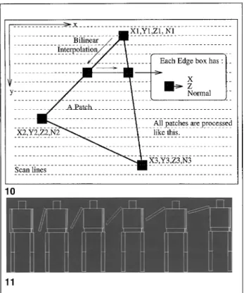
Fig. 10. F o r m a t i o n of the edge boxes in the Z-buffer algorithm Fig. 11. The high degree of coherence in a film

5 Rendering

A comparison of algorithms for the removal of hidden surfaces is found in (Sproull et al. 1974). The Z-buffer algorithm developed by Catmull (1975) combined with the Phong shading model (Phong 1975) represents the most popular rendering scheme. This algorithm, using Sutherland's classification scheme, works on image space or screen space (Fig. 10). The rendering method that MARS uses is the scanline Z-buffer algorithm for the removal of hidden surfaces (Watt 1989). We prefer this algorithm mainly due to its very special nature that perfectly suits our tools for optimizing the rendering process. First it runs on the object space and then the image space. Moreover, it requires much less memory than conventional Z-buffer algorithms that occupy all the screen space for the rendering. The speed of this algorithm is the bottleneck of all the film-making process. If we think of rendering a picture as reducing a 3D scene to a 2D image, then the

rendering of an animated film, i.e., a sequence of frames, is reducing a 4D scene (including time as the fourth dimension) to a 3D image (including time as the third dimension). Thus, rendering an animated sequence of frames must be thought of differently from the rendering of a static scene. If we render a sequence of animated frames separately, i.e., render each frame as totally irrelevant to the others, the result would be acceptable, but there are surely better ways to do this. In terms of efficiency of processing, what makes a sequence of animated film frames different from a sequence of totally irrelevant frames is the concept of temporal coherence (Watt 1989). This is a very important characteristic that can be put to good use.

5. 1 Temporal coherence

The successive frames of any object or joint in an animated film have a great degree of coherence. This is to say, in consecutive frames, an object or a joint makes a relative translation or a rotation to its previous position and orientation (Lasseter 1987). The optimal rendering algorithm should fully exploit the temporal coherence between successive frames in order to reduce the work of rendering. It should avoid rendering the parts of the picture that are identical to those of the previous frame. Such an algorithm should have a mechanism that buffers the parts of the picture that do not change separately from parts of the picture that will change in the next frame. After rendering a frame totally, the next frame can be created by simply rendering only those parts of data that have changed their place and/or orientation since the previous frame. The basis of such an algorithm is that the coherence between successive frames of an animated film is high most of the time (Fig. 11). Temporal coherence is one phe- nomenon exploited fully to render animated film sequences more efficiently.

5.2 Parallelization

In this paper, we investigate the parallel rendering of frames generated by animation on distributed-memory message-passing architectures that are usually referred as multicomputers. In a multicomputer, the processors have only local

(6)

memories, and no memory is shared. In these architectures, synchronization and coordination among processors are achieved through explicit message passing. Multicomputers have been popular due to their nice scalability features. Achieving speed-up through parallelism on such architectures needs special attention. The parallel algorithm must be designed so that both computations and data can be distributed to the processors with local memories in such a way that computational tasks can be run in parallel, while the computational loads of the processors are balanced as much as possible. Communication between processors for exchanging data is necessary, but it is an overhead component of the parallel algorithm that should be minimized for utmost efficiency. Another important factor in designing efficient parallel algorithms is granularity. Granularity depends on both the application and the parallel machine. In a parallel machine with a high communication latency, the program- mer must structure the algorithm so that large amounts of computation are done between communication steps. The implementation described in this work achieves efficient paralMization by considering all these points in designing a parallel rendering algorithm for multicomputers of me- dium-to-coarse grain parallelism.

For the sake of simplicity, we assume that the numbers of inbetween frames in all intervals are always multiples of the number of processors P. Here, an interval refers to a sequence of inbetween frames between two successive keyframes. Hence, each processor can be assigned the rendering of an equal number of inbetween frames in an interval. Inbetween frames are dedicated to individual processors because of the unpredictable computational load involved in the rendering of individual inbetween frames. If the granularity of rendering an inbetween frame is too small, parallel rendering of that frame by P processors may take even longer than simple sequential rendering. In this way, data is processed as if it is compressed between the successive keyframes. However, we can- not compress the data at the keyframes because of the nature of the scheme adopted for exploiting the temporal coherence during the rendering of inbetween frames. All objects are processed during keyframe rendering since stationary and moving parts change partially or completely. Each keyframe is rendered concurrently by all P proces-

sors because the maximum computational load occurs during keyframe rendering.

5.2. 1 Model and film data distribution

The 3D points in space constituting the model database are multiplied by the transformation matrices of the film data for each frame. Hence, both model and film data should be distributed among processors for an efficient parallelization on multicomputers.

Data distribution for keyframe renderings.

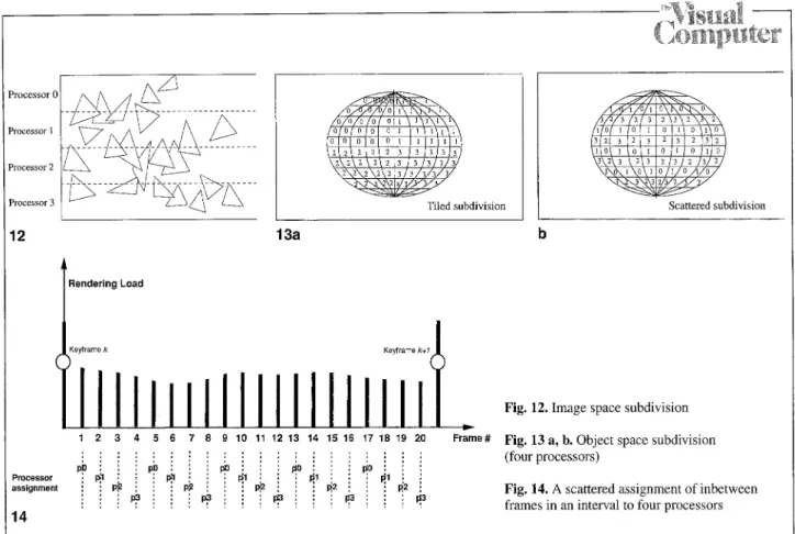
In the parallel rendering of keyframes composed of 3D objects, the distribution of the objects to the processors is a crucial problem in achieving balanced rendering computations. Note that, the model database corresponding to both stationary and moving parts should be distributed to the processors during parallel keyframe rendering. There are two main approaches to this distribution problem: image (screen) space and object-space subdi- visions. In these distribution schemes, objects constituting the model database are treated as lists of patches. In the image-space subdivision, processors are assigned the responsibilities of rendering on disjoint subregions (usually slices) of the over- all screen. Then, the patches are distributed to the processors according to their locations on the view of the scene projected onto the screen (Fig. 12). The advantage of schemes for image space decomposition is the fact that the processors independently construct the final images associated with their slices of the image plane at the end of their local rendering computations. However, computational load balance is a very crucial problem and must be solved in these types of decomposition schemes.

In the object-space distribution schemes, the model database is decomposed evenly into P sub- sets, and the responsibility of rendering each sub- set is assigned to a unique processor. Tiled or scattered decomposition can be adopted for the even decomposition of the whole model database (Fig. 13).

In tiled decomposition, patches belonging to the same objects are supplied consecutively and the successive N mod P processors are assigned the successive patch blocks of size

[N/P~,

whereas the remaining processors are assigned the successive patch blocks of size

[N/P~.

Here, N denotes

(7)

Processor ( Processor I Processor 2 Processor 3 12 Processor assignment 14

G

T i l e d s u b d i v i s i o n 13a

I

Rendering Load Keyirame k+ l 1 2 3 4 5 6 7 8 9 10 11 12 13 14 15 16 17 18 19 20 Frame# ., : : : ,. : : : : ,, : : : : : ,, : : : : p~ ! i ' pi~ i i ' ~ i i ' ~o i i ' r~o i ; ' p:,~l p~ p:'l : p~l P? p.:2 P? p,:2 : :p~ : ~ : : : :: :: ~ : i :: P~. :, :, ~ ~ :~ i 0 .. i i ~ ~ S c a t t e r e d s u b d i v i s i o n

Fig. 12. Image space subdivision

Fig. 13 a, b. Object space subdivision (four processors)

Fig. 14. A scattered assignment of inbetween frames in an interval to four processors

the total number of patches in the model database. In scattered decomposition, patches are assigned to processors in a round robin fashion. That is, the first patch is assigned to the first processor and the second patch is assigned to the second processor, etc. When P patches are assigned, the next patch is assigned to the first processor, and this process continues. In both schemes, the number of patches assigned to the various processors may differ at most by one. However, assigning equal number of patches to each processor does not guarantee a good balance. Different patches may require different rendering times depending on several geometric factors such as their sizes, distances, and orientation to the screen, etc. In scattered decomposition, patches belonging to the same object are shared by various processors. The scattered decomposition is more likely to yield a better load balance than the tiled decomposition since patches belonging to the same object can be assumed to take almost equal rendering time. Thus, scattered decomposition can be considered as a simple yet effective scheme for even object-space distribution. However, parallel rendering algorithms based on object-space decomposition necessitate

global pixel merging after the completion of local rendering computations. Since different processors may produce pixels at the same screen locations, global Z-buffering is required to combine the pixels from each processor into a complete scene. This pixel merging problem introduces a very high computation and communication overhead.

In this work, we divide the conventional algorithm for the removal of scanline Z-buffer hidden surfaces into two phases for the sake of efficient parallelization of keyframe renderings. In the first phase, each patch is passed through a projection pipeline consisting of clipping and edge rasteriz- ation to construct its associated edge boxes on the appropriate scan lines. Note that Z and normal values are also interpolated during edge rasteriz- ation. In the second phase, edge box pairs on scanline lists are processed to render and shade their respective segments. The nice feature of this two-phase approach is the fact that the first phase runs on the object space whereas the second phase runs on the image space. Hence, we exploit this feature by adopting object-space distribution of the model data for the first phase and image-space redistribution of the resulting edge box pairs for

(8)

the second phase. We use a scattered decomposition scheme in the distribution of the model database for the first phase. In spite of the scattered decomposition of the model database, each processor stores its local patches in an object- based hierarchy. This hierarchical storage of sub- sets of local model database is very crucial for maintaining the coherence in the rendering of inbetween frames as will be explained later. The edge box pairs are redistributed in image space after the completion of the first phase of each keyframe rendering, as will also be explained later. The film data requirement for the parallel rendering of each keyframe is only the replication of the identities of the moving objects in the following interval and the transformation matrix corresponding to the last inbetween frame in the previous interval.

Data distribution for inbetween frame render- ing. The rendering of inbetween frames by individual processors necessitates the replication of the model data corresponding only to the moving part(s) among processors for each interval. Note that, the moving part data is to be replicated by its initial positional information for the respective interval. The film data (transformation matrices) corresponding to the moving part(s) in each interval should be distributed among the processors according to the inbetween frame assignments of the processors. The assignment of inbetween frames to individual processors is also a crucial factor for efficient parallelization.

The proposed scheme operates in a synchronous manner. All processors begin to render a keyframe in parallel after completing the rendering of the inbetween frames assigned to them in the previous interval. Those processors completing the rendering of their inbetween frames earlier than the other processors may have to wait idle during the parallel rendering of the following keyframe. There are equal numbers of patches to be rendered in each inbetween frame of a particular interval. However, the rendering complexity of a moving object may vary during its motion. For example, the rendering complexity of an object moving towards (away from) the screen increases (decreases) during its motion due to the increase (decrease) in the projection areas of the patches belonging to that object. However, the rendering complexities of successive inbetween frames can

be assumed to be very close. Hence, we adopt a scattering assignment of inbetween frames to the processors for a better computational balance during the pipelined rendering of inbetween frames. Figure 14 illustrates the scattered assignment of an interval with 20 frames to 4 processors. This figure also illustrates a typical variation of the rendering complexity of a moving object during its motion.

5.2.2 Rendering of keyframes

The object space is subdivided, based on scattered decomposition, only once during the preprocessing phase, and the subdivision is maintained for the parallel first phase computations of all keyframe renderings throughout the whole animation process. Image-space subdivision is repeated for the computations of each keyframe in the second phase. In this work, a scanline is chosen as an atomic process to be performed sequentially by an individual processor. Otherwise, further division of individual scanlines may necessitate an unaccept- able computation and communication overhead in order to maintain spatial coherence. In this work, the number of rendering computations to be performed for each scanline is assumed to be proportional to the number of edge segments which is equal to the (number of edge boxes)/2 on that scanline. Hence, the balanced image-space rendering of the computations in the second phase of keyframe renderings can be formulated as follows: Input instance: We are given n scanlines (s~; s2; ..., s,) with the corresponding computational weights (wl; w2; ... ,wn). Here, wi is taken as the number of edge segments on the scanline si and W is the sum of all wi's.

Problem: These n scanlines must be assigned to P processors so that the sum of the weights of the scanlines mapped to each processor is as close to the optimal load W,verage = W / P as possible. This problem is in fact the number partition- ing problem that is NP-hard. Various heuristics have been proposed for the solution of this problem. In this work we propose a simple yet effective greedy heuristic. The steps of the proposed algorithm for parallel keyframe rendering are given below:

(9)

Step 1: processors concurrently multiply their local 3D points belonging to the moving object(s) in the previous interval by the respective trans- formation matrix in order to compute the final positions of their local patches belonging to those objects. Processors mark these objects as station- ary for the following interval. Then, processors mark the moving objects in the following interval by using their local film data.

Step 2: processors concurrently run the first phase of the scanline Z-buffer algorithm for their local patches. During this operation, each proces- sor constructs two edge lists. One is for its local patches belonging to the stationary objects, and the other is for its local patches belonging to moving objects in the following interval. Note that objects that are going to move in the follow- ing interval are effectively processed according to their initial positions. Meanwhile, each processor constructs a local edge-segment counter (ESC) (an array of size n) where ESC(i) denotes the total number of local edge segments to be rendered on scanline s~ during the second phase. Figure 15 illustrates this operation for a scene with 7 patches and an image plane with 19 scan lines. N o distinc- tion is made between moving and stationary patches, so that only one edge list is shown for the sake of simplicity in illustration.

Step 3: each processor performs a prefix sum on its local ESC array so that ESC(i) holds the total number of local edge segments on the first i scan- lines. Then, a duplicated global vector sum opera- tion is performed on the local ESC vectors. At the end of this global operation, each processor holds a local copy of the ESC array where ESC(i) con- tains the total number of global patches on the first i scanlines. Figure 16 illustrates a sample operation of step 3. The leftmost ESC denotes the local ESC counter of an individual processor. The middle ESC denotes the result of the local prefix sum operation and the rightmost ESC denotes the result of the global sum operation on local ESC arrays.

Step 4: in this step, each processor runs the same mapping heuristic using its own copy of the global ESC array. The proposed heuristic achieves the tiled decomposition of the scanlines by assigning consecutive scanlines from ki-1 + 1 to ki to pro-

s i 6--[Z2X---12~ m s3 m s4 s5 s6 s 7 ~ s j ~ s9 s _ L ~ Sl - sl: ~ Edge-boxes Sl, ~ e-4ZZZZx--4:~ s~ sv

ESC Edgelist Frame Buffer

15 2 2 4 4 4 6 6 8 After 2 prefix-sum 4 4 2 4 10 10 10 8 After global sum 2 4 8 12 16 22 28 361 36! 42 ] 46 ! 48 52 62 72 82 90 E S C m 10 E S C E S C 22 34 pl (72) 52 64 72 100 > 112 p2 (68) 124 140 164 188 p3 (67) 207 234 258 p4 (73) 280 1 6 Wavg = 70

F i g . 1 5 . A n edge list formation with a counter for each line

F i g . 1 6 . Prefix and global sums o f edge segment counters (ESCs)

cessor i for i = 1 , 2 , . . . , P with k o = 0 and ESC(0) = 0, while maintaining the even workload among scanline slices as much as possible. The k indices are determined as follows. Each pro- cessor, after computing ki-a, proceeds on the ESC array starting from ESC(ki_I + 1) until ESC(j) - ESC(ki_ 1) _-> W a v g , where W a v g ~-- W / P =

ESC(n)/P denotes the perfect load balance. Then, k~ is set to j if

E S C ( j ) - E S C ( k ~ _ ~) - - W a v g ~ W a v g - -

(10)

otherwise it is set t o j - 1. The left and right-hand sides of Eq. 1 denote the deviation of the work- loads of processor i from the perfect load balance if scanline slices [ki-1 + 1 . . . j ] or [ki-1 + 1 ... (j - 1)] are assigned to processor i, respectively. Each processor respects this procedure for all processors i = 1, 2, ..., P. Figure 16 illustrates the result of this greedy heuristic for the given ESC array. The numbers inside the parenth- esis denote the number of edge boxes to be processed by the respective processor.

Step 5: at the end of step 4, each processor deter-

mines the mapping information for all scanlines in the image. In this step, each processor sends the edge boxes of the nonlocal scanlines to its home processor according to the mapping information. Then, each processor concatenates (by simple pointer operations) the received edge list with its local edge list.

Step 6: after each processor receives all edge box

data to be rendered on its local scanline slice, it prepares to run the second phase of the rendering algorithm concurrently. Let ni denote the number of scanlines assigned to processor i for i = 0, 1, ... , P - 1 where 2ni = n. Each processor i concurrently allocates and initializes ni x r 2D local arrays, the constant frame buffer (CFB), the constant Z-buffer (CZB), and the local moving Z-buffer (MZB), where r denotes the number of pixels in each scanline. That is, the screen is assumed to contain A = n x r pixels. Here, the CFB and CZB arrays correspond to the respective

scanline slices of their processors. Similarly, the

local moving Z-buffers (MZB) of the processors correspond to their scanline slice assignments. The local CFB and CZB arrays remain constant throughout the intervals, and they are updated at keyframes. Note that two Z-buffers (CZB and MZB) are maintained during keyframe renderings. The local CZB arrays are maintained to keep the Z-values of the pixels produced by stationary parts that will be used to determine the visibility of the moving parts during the succeeding interval. The local MZB arrays are temporary arrays used to determine the visibility of the initial positions of those moving parts on the keyframe. After these local initializations, the processors concurrently carry out the rendering of their local edge segments in two successive phases. In the

first phase, they concurrently render the edge segments belonging to the stationary objects by processing their local stationary edge lists. In this phase, pixels produced by the local edge segments belonging to the stationary parts are Z-buffered with the local CZBs and the resulting Z and pixel values are written into the local CZB and CFB arrays, respectively. This process is straightforward as it is the same as that of the conventional Z-buffer algorithm. In the second phase, processors concurrently render the edge segments belonging to the moving objects (in the next interval) by processing their local moving edge lists. How- ever, the process in this phase is slightly different from the conventional sequential Z-buffer algorithm. The pixels produced by the local edge segments belonging to the moving objects are Z- buffered with both local MZBs and CZBs. The resulting Z-values are written into the local MZBs whereas the resulting pixel values are written into the local CFBs. Although the local CZB arrays are used for Z-buffering, they are not modified at all during this phase. Thus, the Z-values of the pixels produced by stationary parts are not lost and the local CZBs can be exploited to realize the temporal coherence during inbetween frame renderings. At the end of this step, processors deallocate their MZB arrays.

Step 7: At the end of step 6, the local CFBs

contain the final images of an individual keyframe on the respective screen slices. The processors send their local CFBs to the host for display. Then processors concurrently run a global concatenation on their local CZB arrays. At the end of this global operation, each processor gets a copy of the global constant Z-buffer (GCZB) array of size n x r. Similarly, the processors concurrently run a global concatenation on their local patches belonging to the moving objects in order to replicate the moving part database in each processor. This is done for the inbetween frame rendering in the next interval. At the end of this step, the processors deallocate their local CZB arrays.

5.2.3 Rendering of inbetween frames

The processors maintain two local moving frame buffers (MFB) and MZB arrays of size n x r for inbetween frame renderings. These arrays are

(11)

static and are re-initialized just before each inbetween frame rendering. Recall that each processor also holds a local copy of the GCZB which con- tains the Z-values of the pixels produced by the objects that stay stationary during the respective interval.

The processors concurrently multiply the 3D points of the moving object(s) with different transformation matrices using their local film data. Then, they concurrently and independently render the moving objects in different positions that are c o m p u t e d locally. Hence, P successive inbetween frames are rendered concurrently. During these local rendering computations, the processors compare the Z-values of the pixels produced by the moving object(s) with their local M Z B and GCZB arrays and write the resulting Z and pixel values into their local M Z B and M F B arrays. Local copies of the GCZB array remain intact since they are needed for their rendering of other inbetween frames in the same interval. Each processor sends its local M F B array to the host for display u p o n completing the rendering of an inbetween frame. Then, it repeats this procedure for the next inbetween frame assigned to it. N o interprocessor communication is involved in the inbetween frame rendering except the transmissions of the resulting M F B arrays to the host.

5.2.4 How the host interprets the image data

coherence in the incoming data, the use of blocks instead of single pixels for flagging is efficient. The only issue in this mechanism is how large the blocks should be. If they are too large, un- necessary time will be spent in writing the background buffer back to the screen. If they are too small, overheads in comparison will be introduced.

5.2.5 Performance results and conclusion

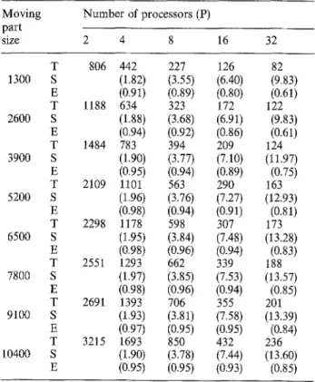
The performance of the parallel rendering of the animation data generated by MARS is tested on an Intel iPSC/2 Hypercube with 32 processors. Table 1 illustrates the execution times for the parallel rendering of inbetween frames of an animation data for various numbers of processors and various sizes of moving parts. The data in Table 1 correspond to the averages of various types of movement of a number of segments (out

Table 1. Variation of the execution times (T in ms), speed-ups (S), and efficicncies (E) with respect to two processors of the parallel rendering of inbetween frames for the animation of a model (with eight segments and 10400 patches) with the number of processors and moving part sizes.

Moving part size Number of processors (P) 2 4 8 16 32 T 806 442 227 126 82 1300 S (1.82) (3.55) (6.40) (9.83)

At each keyframe, the host receives a CFB. It E (0.91) (0.89) (0.80) (0.61) writes this buffer on the screen. Then it receives T 1188 634 323 172 122

2600 S (1.88) (3.68) (6.91) (9.83)

consecutive MFBs. To write a M F B on the screen, E (0.94) (0.92) (0.86) (0.61)

the host first must copy the pixels that will be T 1484 783 394 209 124 occupied by the M F B pixels. The background is 3900 s (1.90) (3.77) (7.10) (11.97) saved because the host will write it back before E (0.95) (0.94) (0.89) (0.75)

T 2109 1101 563 290 163

writing the moving parts of the next frame. Due to 5200 s (1.96) (3.76) (7.27) (12.93)

the nature of the problem, we need a background- E (0.98) (0.94) (0.91) (0.81) saving mechanism for the M F B writing. The solu- T 2298 1178 598 307 173 tion to this problem works as follows. We hold the 6500 s (1.95) (3.84) (7.48) (13.28)

E (0.98) (0.96) (0.94) (0.83)

received CFB after writing it on the screen as T 2551 1293 662 339 t88 a background buffer. We also hold a 2D binary 7800 s (1.97) (3.85) (7.53) (13.57) array, where each bit denotes whether a block of E (0.98) (0.96) (0.94) (0.85)

T 2691 1393 706 355 201

pixels is overwritten or not. That is, as we write 9100 s (1.93) (3.81) (7.58) (13.39)

any pixel of the M F B on the screen, we set the B (0.97) (0.95) (0.95) (0.84)

corresponding bit to 1. Then, before writing a new Y 3215 1693 850 432 236 MFB, the blocks of pixels with flags set are writ- 1o4oo s (1.90) (3.78) (7.44) (13.60) ten on the screen. As long as there is spatial E (0.95) (0.95) (0.93) (0.85)

(12)

of 8 segments) with 32 inbetween frames. Uni- processor execution times are not obtained due to insufficient memory. The speed-up and efficiency values illustrated in Table 1 (in parentheses) denote the speed-up and efficiency values for 4, 8, 16, and 32 processors with respect to 2 processors. Scanning individual rows of Table 1 reveals that speed-up increases whereas efficiency decreases with an increasing number of processors for a fixed size of moving parts. The low efficiency values in the last column (P = 32) of Table 1 re- veal the load imbalance among the rendering of inbetween frames (only one inbetween frame is assigned to an individual processor for P = 32). However, considerably larger efficiency values in other columns (P = 4, 8, 16) confirm the expected high performance of the scattered assignment of inbetween frames to processors. The increase in the efficiency values with a decreasing number of processors (P = 16, 8, 4) for a fixed size of moving part confirms the increase expected in the performance of the scattered assignment with an increasing number of inbetween frames (2, 4, 8) assigned to an individual processor. As is seen from Table 1, scattered assignment yields suffi- ciently high efficiency even for 2 inbetween frames per processor (column P = 16). Furthermore, scanning individual columns (P = 4, 8, 16) of Table 1 illustrates that speed-up and efficiency values with respect to two-processors increase in general with increasing size of moving parts. This increase is attributed to two factors. The first is the granularity increase with increasing size of moving parts. The communication overhead due to the transmission of individual moving part images to the host is proportional to the screen size. However, computational times of inbetween

frame renderings increase with increase in moving part sizes. The second factor that may contribute to this increase in the efficiency is the better load balance with increasing part sizes. In Table 1, the increase in moving part size is realized by increasing the number of moving segments. Hence, different motions of multiple segments may yield a better computational balance among various inbetween frame renderings.

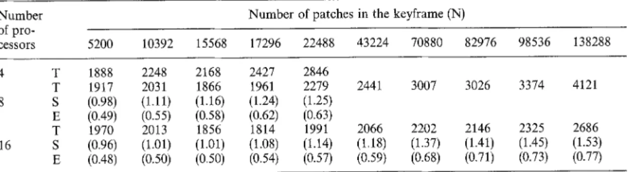
Table 2 illustrates the execution times for the parallel rendering of keyframes of various animation data of various sizes on different number of processors. Execution times for one, two and four processors for N > 43224 were not obtained due to insufficient memory. Speed-up and efficiency values on a particular row P = 8 (N > 43224) and 16 in Table 2 denote the speed-up and efficiency values with respect to the

P/2

= 4 and 8 processors, respectively, for the respective keyframe sizes. As is seen in the first column of Table 2, speed-down occurs for the smallest keyframe size (N = 5200) when we double the number of processors (i.e., from 4 to 8 and from 8 to 16). How- ever, we always obtain a speed-up for larger keyframe sizes (N > 10392) and speed-up and efficiency values monotonically increase with increasing keyframe sizes. Recall that the proposed parallel algorithm has two overhead components. The first one is the computation and communication overhead introduced during the parallel load rebalancing after the parallel formation of local edge lists (steps 3 and 4). The second one is the communication overhead due to the transmission of local CFBs to the host at the end of the parallel rendering of keyframes (step 7). An additional overhead is the global concatenation of the local CZB array at step 7. The first overhead is a

Table 2. Variation of the execution times (T in ms), speed-ups (S) and efficiencies (E) with respect to P/2 processors of the parallel rendering of the keyframes with the number of processors and data sizes.

Number Number of patches in the keyffame (N)

of processors 5200 10392 15568 17296 22488 43224 70880 82976 98536 138288 4 T 1888 2248 2168 2427 2846 T 1917 2031 1866 1961 2279 2441 3007 3026 3374 4121 8 S (0.98) (1.11) (1.16) (1.24) (1.25) E (0.49) (0.55) (0.58) (0.62) (0.63) T 1970 2013 1856 1814 1991 2066 2202 2146 2325 2686 16 S (0.96) (1.01) (1.01) (1.08) (1,14) (1,18) (1.37) (1.41) (1.45) (1.53) E (0.48) (0.50) (0,50) (0.54) (0.57) (0.59) (0.68) (0.71) (0.73) (0.77)

(13)

function of the total number of scanlines and the diameter of the interconnection topology of the parallel architecture (i.e., log2P in the hypercube). That is, the first overhead does not increase with increasing keyframe size. Similarly, the second and the third overhead components are only proportional to the screen size. The percentage of the overhead (overhead time/total parallel rendering time) decreases with increasing keyframe size (N), resulting in increasing speed-up and efficiency values with increasing N. As is seen in Table 2, we obtain a speed-up of 1.53 (an efficiency of 0.77) for the largest size of keyframe when we double the number of processors from 8 to 16. The proposed parallel algorithm is expected to yield a much better performance for larger keyframe sizes and parallel architectures with lower communication/computation ratios (e.g., fine grain architectures).

Acknowledgements. This project is supported by the following grants and funds: Bilkent University Research Funds. Research Grant MAG917-EEEAG5 of the Scientific and Technical Research Council of Turkey, Intel Corporation Grant SSD100791-2

References

Badler NI (1986) Animating human figures: perspectives and directions. Proc Graphics Interface & Vision Interface, Toronto, Ontario, pp t15-120

Badler NI (1987) Articulated figure animation. IEEE Comput Graph Appl 7:10~11

Badler NI, Manoochehri KH, Baraff D (1986) Multi-dimensional input techniques and articulated figure positioning by multiple constraints. Workshop on Interactive 3D Graphics, New York, pp 151-169

Badler NI, Manoochehri KH, Walters G (1987) Articulated figure positioning by multiple constraints. IEEE Comput Graph Appl 7:28-38

Blinn JF (1987) Nested transformations and blobby man. IEEE Comput Graph Appl 7:59-65

Cachola DG, Schrack G F (1986) Modelling and animating three-dimensional articulate figures. Proc Graphics Interface & Vision Interface, Toronto, Ontario, pp. 152 157

Catmull E (1975) Computer display of curved surfaces. In Proc IEEE Conference on Computer Graphics, Pattern Recogni- tion and Data Structures, p 11

Farin G (1990) Curves and Surfaces for Computer Aided Geo- metric Design. Academic Press, Boston

Getto P, Breen D (1990) An object-oriented architecture for a computer animation system. Visual Comput, 6:7942 Girard M (1987) Interactive design of 3D computer-animated

legged animal motion. IEEE Comput Graph Appl 7: 131-149

Grosso MR, Badler NI, Quach RD (1989) Anthropometry for computer graphics human figures. Technical report, Univer- sity of Pennsylvania, Philadelphia

Heller D (1990) X View Programming Manual 2n edn. O'Reilly & Associates, California

Hewitt S, Ridscale G, Calvert TW (1986) The interactive specification of human animation. Proc Graphics Interface & Vi- sion Interface, Toronto, Ontario, pp 121-130

Jackson AW, Morris JM (1988) Enhancement of diglib: computer graphics software for animated computer-generated video movies. Comput Graph 12:271 283

Lasseter J (1987) Principles of traditional animation applied to 3D computer animation. Comput Graph 21:35-44

Magnenat-Thalmann N, Thalmann D (1985) Computer Anima- tion, Theory and Practice. Springer, Berlin Heidelberg New York

Mahmud SK, Ozgtiq B (1990) Human body animation. Proc Fifth International Symposium on Computer and Informa- tion Science, Nev~ehir, Turkey, pp. 885-894

Mahmud SK, Ozgii~ B (1991) Semi goal-directed animation: a new abstraction of motion specification in parametric keyframe animation of human motion. Proc Second Euro- graphics Workshop on Animation and Simulation, Vienna, pp 75-87

Ostby EF, Reeves WT, Leftter SJ (1990) The menv modelling and animation environment. J Visualization & Comput Anim,

1:33-40

Ozgfi9 B (1988) Thoughts on user interface design for multi window environments. In Proc Second International Sympo- sium on Computer and Information Science, Istanbul, pp 477-488

Phong B-T (1975) Illumination for computer generated pictures. Commun ACM, 18:311-317

Rogers D F (1989) Mathematical Elements for Computer Graphics. McGraw Hill, New York

Rogers D F (1990) Procedural Elements for Computer Graphics. McGraw Hill, New York

Shoemaker K (1985) Animating rotation with quaternion curves. Proc SIGGRAPH, pp 245-254

Sprouli RF, Sutherland IE, Schumacker RA (1974) A character- ization of ten hidden surface removal algorithms. ACM Com- put Surveys, 6:1-55

Tokad Y (1990) Analysis of Engineering Systems. Bilkent Uni- versity, Ankara

Watt A (1989) Fundamentals of Three-dimensional Computer Graphics. Addison-Wesley, Massachusetts

Wyvill B, Chmilar M, Herr C (1991) A software architecture for integrating modeling with kinematic and dynamic animation. Visual Comput 7:122-137

MURAT AKTIHANO~LU

works at Computer Services, Inc., Tampa, Florida. His research interests are in computer graphics, animation and related parallel algorithms.

Aktihano~lu received his B.S. degree in electronic and electrical engineering, and his M.S. degree in computer engineering and information science, both from Bilkent University, in 1990 and 1993, respectively.

(14)

BULENT {~)ZGOC joined Bilkent University, Faculty of Engineering in 1986. He is currently a university professor of computer science and the dean of the Faculty of Art, Design and Architecture. He formerly taught at the University of Pen- nsylvania, Philadelphia College of Arts, Middle East Technical University and worked as a member of research staff at the Schlumberger Palo Alto Re- search Center. For the last fif- teen years, he has been active in the field of Computer graphics and animation.

Ozgfi~ received his B. Arch. and M. Arch. degrees in architecture, both from Middle East Technical University, Ankara, Turkey, in 1972 and 1973, respectively. He received his M.S. degree in architectural technology from Columbia University, and his Ph.D. degree in a joint program of architecture and computer graphics from the University of Pennsylvania, in 1974 and 1978 respectively. He is a member of ACM Siggraph, IEEE Computer Society and UIA.

'CEVDET AYKANAT joined the department of Computer Engineering and Information Science, Bilkent University in 1988 where he is currently an associate professor. Formerly, he worked at the Intel Super- computer System Division, Bea- verton, as a research associate. His research interests include parallel processing, parallel computer graphics applications, and non-deterministic optimiza- tion techniques.

Aykanat received his B.S. and M.S. degrees from Middle East Technical University, Ankara, Turkey, and his Ph.D. degree from the Ohio State University, Columbus, all in electronic and electrical engineering. He was a Fulbright scholar during his Ph.D. studies.