Contents lists available atScienceDirect
Automatica
journal homepage:www.elsevier.com/locate/automatica
Brief paper
Foraging motion of swarms with leaders as Nash equilibria
✩Aykut Yıldız
1,
A. Bülent Özgüler
Electrical and Electronics Engineering Department, Bilkent University, Ankara 06800, Turkey
a r t i c l e i n f o
Article history:
Received 15 September 2015 Received in revised form 16 June 2016
Accepted 22 June 2016
Available online 5 September 2016 Keywords: Leader–follower Rendezvous problem Ordered graph Directed star Nash equilibrium Swarm Foraging Multi-agent systems Differential game theory
a b s t r a c t
The consequences of having a leader in a swarm are investigated using differential game theory. We model foraging swarms with leader and followers as a non-cooperative, multi-agent differential game. The agents in the game start from a set of initial positions and migrate towards a target. The agents are assumed to have no desire, partial desire or full desire to reach the target. We consider two types of leadership structures, namely hierarchical leadership and a single leader. In both games, the type of leadership is assumed to be passive. We identify the realistic assumptions under which a unique Nash equilibrium exists in each game and derive the properties of the Nash solutions in detail. It is shown that having a passive leader economizes in the total information exchange at the expense of aggregation stability in a swarm. It turns out that, the leader is able to organize the non-identical followers into harmony under missing information.
© 2016 Elsevier Ltd. All rights reserved.
1. Introduction
There are certain advantages of having a leader in a swarm. The leader may initiate the route and the remaining group mem-bers follow that path (Estrada & Vargas-Estrada, 2013). Therefore, leader designates the search direction (Wang & Wang, 2008). By leader guidance, a wider area can be covered and the collisions can be avoided (Wang & Wang, 2008). Moreover, leader–follower swarms reach consensus more rapidly (Estrada & Vargas-Estrada, 2013). There are also cases, where consensus may not even be guaranteed by only simple rules and choices of specific leaders be-come necessary to ensure consensus (King & Cowlishaw, 2009). Leadership also provides orientation improvement and coordi-nation via communication in the group (Andersson & Wallan-der, 2004;Weimerskirch, Martin, Clerquin, Alexandre, & Jiraskova, 2001). Leader–follower swarms have a multitude of practical ap-plications such as robot teams, ship flocks, UAVs, and vehicle
pla-✩ This work is supported in full by the Science and Research Council of Turkey (TUBITAK) under project no. EEEAG-114E270. The material in this paper was not presented at any conference. This paper was recommended for publication in revised form by Associate Editor Michael M. Zavlanos under the direction of Editor Christos G. Cassandras.
E-mail addresses:[email protected](A. Yıldız),
[email protected](A.B. Özgüler). 1 Fax: +90 312 266 4192.
toons. The leader may play various roles in such systems. In robot teams, a leader is generally an active one, who itself is motion-controlled by an external control input (Kawashima & Egerstedt, 2014). In ship flocks, leader may enable coordination of possibly under-actuated followers (Lapierre, Soetanto, & Pascoal, 2003). In unmanned aerial vehicles, leader may provide reference position and velocity for followers (Karimoddini, Lin, Chen, & Lee, 2013). In vehicle platoons, leader ensures string stability where tight for-mations are maintained (Peters, Middleton, & Mason, 2014). In optimization techniques such as PSO, leader usually follows the shortest path, i.e., the line towards the minimum and the fol-lowers perform the search around that line (Chatterjee, Goswami, Mukherjee, & Das, 2014). In all these systems, leaders constitute a small subset of the group that guides the coordination of the whole network (Estrada & Vargas-Estrada, 2013).
We strive to understand the mechanisms of spontaneous formation of swarms via dynamic non-cooperative game theory of Basar and Olsder(1995) and necessary conditions of optimality of Kirk(2012). We define ‘‘spontaneous formation’’ as the formation of collective behavior based on non-cooperative decisions. Nash equilibrium is ideally suited to model such mechanisms. In Nash equilibrium, each agent gives a best response to the decisions of other agents which results in a collective behavior. We use a game theoretical model and ask whether such equilibrium exists. It turns out that the Nash solution exists and is unique for continuous strategies and for the information structures studied here. http://dx.doi.org/10.1016/j.automatica.2016.07.024
The difficulty of establishing the existence of Nash equilibria in dynamic multi-agent games with non-convex cost functions is well known (Bressan & Shen, 2004). This continues the quest inÖzgüler and Yıldız(2013) andYıldız and Özgüler(2015), in which, the ex-istence and uniqueness of two swarm games were successfully shown under some realistic assumptions on the information struc-ture among group members and on the allowed strategies to the agents. Here, we focus on passive leaders that are singled out by the other agents, not because they command, coordinate, or organize, but because of their present geographical position in the group. We study two information structures that define games with passive leaderships. The first structure corresponds to an ‘‘ordered graph’’, Chvátal(1984), and here it is referred to as hierarchical leadership. The second structure corresponds to a ‘‘directed star’’ graph, Col-bourn, Hoffman, and Rodger(1991), and here it is referred to as single leadership. In both games, the swarm members are allowed to be ‘‘non-identical’’ and each member measures its distance only to those members that are ahead. Both games may be compared with the v-formation of birds (although we limit our study to one-dimensional swarms) because an agent’s (level of) leadership de-pends on how close it is to the top of the hierarchy,Nagy, Ákos, Biro, and Vicsek(2010) andWang and Wang(2008). These games have a loose information structure as very little amount of atten-tion span is needed from an agent during its journey. One conse-quence of this sparsity in intra-swarm communication is economy in energy expenditure. Power and energy expenditure reduction is indeed an essential feature of v-formation (Cutts & Speakman, 1994;Hainsworth,1988;Weimerskirch et al.,2001), and ( Speak-man & Banks, 1998).
The swarming models introduced in this article offer significant improvements over (Özgüler & Yıldız, 2013; Yıldız & Özgüler, 2015). Current models cover non-identical agents, which extends the identical agent structure of Özgüler and Yıldız (2013) and Yıldız and Özgüler(2015). Also, in the current model, the agents act with position information of only the forward agents. Ordered graph and directed star information structures used here are less restrictive than those in Özgüler and Yıldız (2013) and Yıldız and Özgüler (2015). Note that, neither of the four information structures (the ones here and those inÖzgüler and Yıldız(2013) andYıldız and Özgüler(2015)) is a special case of the remaining three.
The paper is organized as follows. Section 2 contains the definitions of the games considered, the individual cost functions that model the motive of each agent and their interpretation as the total effort of an agent in the foraging journey. In Section3, the main results, the existence and uniqueness of a Nash solution, and its features that relate to a swarming behavior are listed. In Section5, we discuss the necessity of the constraints posed in the definitions of the games. In Section4, four swarm games that have Nash solutions are compared. Section6is on conclusions. Detailed proofs ofTheorems 1and2are given on the web page (Yıldız & Özgüler,2016).
2. Two games with leader–follower structure
The games defined are based on motives of a group of agents under two different hypotheses on information structure. In both games, when the agents are assumed to be foraging, say, for food, they start from some initial positions and try to migrate towards a target location. In cases of foraging or non-foraging, and also with or without specified target location, we would like to show that the non-cooperative motives of the agents lead to a collective behavior dictated by a Nash Equilibrium of the games, whenever it exists.
Game L1 (Hierarchical Leadership): Determine minui
{
Li}
subjectto
˙
xi=
ui, ∀
i=
1, . . . ,
N, where L1:=
γ
x 1(
T)
2 2+
T 0 u1(
t)
2 2 dt,
Li:=
β
x i(
T)
2 2+
T 0
ui(
t)
2 2+
i−1
j=1
aj[
xi(
t) −
xj(
t)]
2 2−
rj|
xi(
t) −
xj(
t)|
dt,
2≤
i≤
N.
(1)Game L2 (Single Leader): Determine minui
{
Li}
subject to˙
xi=
ui
, ∀
i=
1, . . . ,
N, where L1:=
γ
x 1(
T)
2 2+
T 0 u1(
t)
2 2 dt,
Li:=
β
x i(
T)
2 2+
T 0
ui(
t)
2 2+ ¯
ai[
xi(
t) −
x1(
t)]
2 2− ¯
ri|
xi(
t) −
x1(
t)|
dt,
2≤
i≤
N.
(2)In both games, L1is the cost minimized by one agent and Li
,
i=
2, . . . ,
N, are the costs minimized by the others, where N is the swarm population. The swarming duration is specified as T>
0, ui(
t) = ˙
xi is the control input, and xi(
t)
is the position at timet
∈ [
0,
T]
of the ith agent. The adhesion aj>
0 is an attraction parameter and rj>
0 is a repulsion parameter. Parametersγ ≥
0 andβ ≥
0 weigh the foraging efforts; the higher they are, the bet-ter is the desire to reach foraging target by the respective agent. The agents control their velocities to minimize their total effort, which consists of kinetic energy ui(
t)
2as well as the artificialpo-tential energy. Here, combined attractive, repulsive, and foraging terms in the cost function of an agent is interpreted as the artificial potential energy of that agent,Gazi and Passino(2004).
The exact foraging target is normalized to be the origin in x1
(
T) . . .
xN(
T)
-space. The agents may have varying degrees of de-sires to reach this target in Games L1 and L2. The foraging task is performed through the presence of the foraging terms with weightsγ
andβ
in the cost functions since their minimization will imply that an agent is as close to the origin as possible. If these terms are removed from the cost functions and, instead, the termi-nal conditions x1(
T) =
0, . . . ,
xN(
T) =
0 are required, then this is a slightly different game and will be referred to as the specified ter-minal condition game. If x1(
T), . . . ,
xN(
T)
are altogether free, then there is no foraging requirement and the corresponding slightly different games (in which the foraging terms are simply removed from the cost functions) will be called the free terminal condition games.The cost functions considered in this game are similar to those inÖzgüler and Yıldız(2013) andYıldız and Özgüler(2015) with important differences. In all games, the indexing of the agents in-dicate the ranking in the initial queue of the agents. The agent of index 1 starts at the closest position to the foraging target and that with index N, to be at the farthest. Here, agent-1 and others have different cost function structures, as opposed to the uniform struc-ture inYıldız and Özgüler(2015). Second, we extend the identi-cal agent form ofYıldız and Özgüler(2015) to non-identical agents by allowing coefficients a and r to vary among different agents who have no desire, partial desire, or full desire to reach the tar-get. Above all, we alter the self organized structure inÖzgüler and Yıldız(2013) andYıldız and Özgüler(2015) to a leader–follower structure. The agent of index 1 is distinguished by its ignorance of the position of any other member in the group in the duration of the whole journey. Each agent in Game L1 is assumed to ob-serve (measure) and know the positions of the agents ahead of
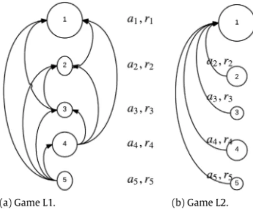
it, whereas in Game L2, it is assumed to observe the position of agent-1 only. The latter is the loosest information structure among those inÖzgüler and Yıldız(2013) andYıldız and Özgüler(2015), Game L1, and Game L2. One way to view Game L1 is that each agent exhibits a different level of leadership based on its rank in the swarm. In other words, all the agents except the rearmost agent perform leadership by being under surveillance by the agents at its back. The agent in front is a full leader relied upon by all remaining agents in Game L2. Therefore, the passive leadership is somewhat hierarchical in the first case, whereas one distinguished agent is the passive leader and all others are followers in the latter case. The information structures of these two games are illustrated in Fig. 1. An arrow emanating from agent-i to agent-j indicates that i keeps track of its distance to j during the foraging journey.
Solving the games via minimizing the inter-dependent non-convex cost functions in(1)and(2)is challenging due to several reasons. While it is relatively easy to transform the problems posed by Games L1 and L2 into problems of finding solutions to systems of differential equations, these are nonlinear and unfortunately do not obey any Lipschitz conditions. A further difficulty is that these systems have mixed boundary conditions. We are able to surmount these difficulties, only because a postulate on the ranking of the agents in the queue during the whole journey eliminates the nonlinearity of the system. Of course, this postulate, in turn, needs to be verified by the solutions obtained; a task that is sometimes doable.
3. Main results
We now summarize the main results for Games L1 and L2 under three different specification schemes on the foraging target and list their implications in relation to the swarming behavior.
3.1. Nash solution for Game L1 Let
α
1:=
0,α
k:=
√
a1
+ · · · +
ak−1,
k=
2, . . . ,
N be calledconvergence rates for Game L1 and suppose that xN
(
0) > · · · >
x1
(
0)
. Defineρ
j(
t) :=
γ − β
γ
T+
1
sinh(α
j+1t)
β
sinh(α
j+1T) + α
j+1cosh(α
j+1T)
,
j=
1 0,
j=
2, . . . ,
N,
bk(
t) :=
1−
γ
tγ
T+
1,
k=
1β
sinh[
α
k(
T−
t)] + α
kcosh[
α
k(
T−
t)]
β
sinh(α
kT) + α
kcosh(α
kT)
,
k=
2, . . . ,
N,
ck(
t) :=
1α
2 k
1−
bk(
t) −
β
sinh(α
kt)
β
sinh(α
kT) + α
kcosh(α
kT)
,
k=
2, . . . ,
N.
(3)Theorem 1. There exists a unique Nash equilibrium for the
hierar-chical leadership game under continuous strategies if and only if
γ ≥
β ≥
0. The Nash equilibrium has the following features:P1. The initial ordering among the agents is preserved during 0
≤
t≤
T .P2. The leader trajectory and the distances to the leader are given by x1
(
t) =
b1(
t)
x1(
0),
xi(
t) −
x1(
t) = ρ
1(
t)
x1(
0) +
i
k=2{
bk(
t)[
xk(
0) −
xk−1(
0)]
+
ck(
t)
rk−1}
,
2≤
i≤
N.
(4)(a) Game L1. (b) Game L2.
Fig. 1. Information structures of two swarm games.
P3. The swarm size is given by
|
xN(
t) −
x1(
t)| = ρ
1(
t)|
x1(
0)|
+
N
k=2{
bk(
t)|
xk(
0) −
xk−1(
0)| +
ck(
t)|
rk−1|}
.
P4. The swarm center xc
:=
(
1/
N)(
x1+ · · · +
xN)
follows the trajectory xc(
t) =
b1(
t)
x1(
0) + ρ
1(
t)
x1(
0)
+
1 N N
i=1 i
k=2{
bk(
t)[
xk(
0) −
xk−1(
0)] +
ck(
t)
rk−1}
,
t∈ [
0,
T]
.
P5. If the foraging target is specified for all agents including the followers, then there is a unique Nash equilibrium of Game L1 for continuous strategies. The distance expressions are obtained from(4)in the limit as
γ , β → ∞
in(3).P6. If the foraging task is dropped, then there still exists a unique Nash equilibrium for continuous strategies. The distance expressions are obtained by(4)by substituting
γ =
0 andβ =
0 in(3).Remark 1. (i) Note that the Nash solution is valid when
β =
0and
γ ≥
0. If in additionγ >
0, then this is the case in which only the leader has a desire to reach the foraging target. Ifγ =
0, then there is no foraging task at all, which is the situation considered by P6. In case there is no foraging task, then the leader’s optimal trajectory is x1(
t) =
x1(
0) ∀
t∈
[
0,
T]
, i.e., the leader preserves its initial position at all times. In the resulting Nash equilibrium, other agents progressively get closer to the leader in time.(ii) The necessity of
γ ≥ β
, i.e., the foremost leader having more desire to reach the foraging target is quite intuitive since otherwise, under certain initial conditions, the agent of index 1 will fall behind. However, agent of index 1 does not observe its distance to the other agents so that a consensus (a swarm) is not formed at all. This is illustrated inYıldız and Özgüler (2016) where the leader is overtaken by the followers so that a Nash solution does not emerge.(iii) If adhesion increases as aj
→ ∞
for all j=
1, . . . ,
N, then all agents instantaneously stick to each other and move towards the target location altogether.(iv) Under constant adhesions, if rj
→ ∞
for all j=
1, . . . ,
N, then the agents suddenly depart from each other, stay in that location until the final time T and suddenly move towards the target location as t→
T as the foraging terms becomes more effective in the cost functions.(v) If the target is specified to all agents (
γ , β → ∞
), then starting at any set of initial positions, all agents end up precisely at the foraging target. Ifγ → ∞
andβ =
0, then the followers still move towards the target location, but do not end up exactly at the target.3.2. Nash solution for Game L2
Let
α
¯
k:=
√
ak, which will figure as convergence rates for Game L2, and suppose that xi(
0) >
x1(
0)
for 1<
i≤
N. Define¯
ρ
k(
t) =
γ − β
γ
T+
1
sinh( ¯α
k+1t)
β
sinh( ¯α
k+1T) + ¯α
k+1cosh( ¯α
k+1T)
,
k=
1, . . . ,
N−
1,
¯
ck(
t) :=
1¯
α
2 k
1− ¯
bk(
t) −
β
sinh( ¯α
kt)
β
sinh( ¯α
kT) + ¯α
kcosh( ¯α
kT)
,
k=
2, . . . ,
N,
(5)¯
bk(
t) :=
1−
γ
tγ
T+
1,
k=
1β
sinh[ ¯
α
k(
T−
t)] + ¯α
kcosh[ ¯
α
k(
T−
t)]
β
sinh( ¯α
kT) + ¯α
kcosh( ¯α
kT)
,
k=
2, . . . ,
N.
(6)Theorem 2. There is a unique Nash equilibrium for single leader
game under continuous strategies if and only if
γ ≥ β ≥
0. The Nash equilibrium has the following properties:P1. The Agent-1 remains the leader throughout the journey. There are initial conditions that lead to legitimate ordering changes among the agents unless ai
=
a for all i=
2, . . . ,
N.P2. The leader trajectory and distances of the followers to the leader are given by
x1
(
t) = ¯
b1(
t)
x1(
0),
xi
(
t) −
x1(
t) = ¯ρ
i−1(
t)
x1(
0) + ¯
bi(
t)[
xi(
0) −
x1(
0)]
+ ¯
ci(
t)¯
ri 2≤
i≤
N.
(7)
P3. An upper bound on the swarm size d
(
t)
is given by d(
t) ≤
max i{ ¯
ρ
i−1(
t)}|
x1(
0)| +
max i{¯
bi(
t)|
xi(
0) −
x1(
0)|}
+
max i{¯
ci(
t)¯
ri}
.
P4. The swarm center xc
=
(
1/
N)(
x1+· · ·+
xN)
follows the trajectoryxc
(
t) = ¯
b1(
t)
x1(
0) +
1 N N
i=1{ ¯
ρ
i−1(
t)
x1(
0) + ¯
bi(
t)[
xi(
0) −
x1(
0)]
+ ¯
ci(
t)¯
ri}
,
t∈ [
0,
T]
.
P5. If the foraging target is specified for all agents including the followers, then there is a unique Nash equilibrium of Game L2 for continuous strategies. The distance expressions are obtained from(7)in the limit as
γ , β → ∞
in(5).P6. If the foraging task is dropped, then there still exists a unique Nash equilibrium for continuous strategies. The distance expressions are obtained by(7)by substituting
γ =
0 andβ =
0 in(5).Remark 2. (i) In this loose information structure, a unique Nash
equilibrium is still reached if and only if the leader has more desire to reach the target location (
γ ≥ β
).(ii) The ordering in the resulting swarm is such that the leader maintains its position at all times. On the other hand, changes of ordering among followers are permissible in this Nash equilibrium.
(iii) Ifa
¯
i=
a andr¯
i=
r for all i=
2, . . . ,
N, then no ordering change occurs among the agents since Game L2 becomes a special case of Game L1.(iv) The trajectory dynamics in Game L2 (under all three types of target specification) are always dominated by hyperbolic functions. This is a consequence of the hypothesized types of the artificial energy components in the cost functions(1)and (2)as well as the dynamic constraint. In fact, the same kind of dynamics dominate the other trajectories resulting in Game L1 as well as in Games 1 and 2.
(v) If adhesion is large such thata
¯
i→ ∞
for some i∈ {
1, . . . ,
N}
, then agent i instantaneously sticks to the leader and moves towards the target location with the leader.(vi) Ifr
¯
i→ ∞
for some i∈ {
1, . . . ,
N}
, then the agent i suddenly departs from the swarm, stays there until the final time T and suddenly moves towards the target location as t→
T when the foraging term becomes more effective in the cost functions.(vii) In both Games L1 and L2, if some agents are initially at the same position, then the Nash solution is such that they maintain the same position during the whole journey.
4. Comparison of nash equilibria in four games of swarm
The two games considered here and the earlier swarm games ofÖzgüler and Yıldız(2013) andYıldız and Özgüler(2015) will now be compared focusing on the Nash equilibria that result. We compare only the specified terminal condition versions of these four games. This is merely for convenience since under specified target location, the trajectories end up exactly at x1
(
T) =
0, . . . ,
xN(
T) =
0 so that the resulting trajectory expressions are all more compact. Same analyses and conclusions are also valid when the agents have a partial desire (free terminal condition) or no desire (unspecified terminal condition) to reach target location. Let us define the game inÖzgüler and Yıldız(2013) as Game 1, and the game inYıldız and Özgüler(2015) as Game 2. The first significant difference of the four games; Game 1, 2, L1, and L2 is that the initial ordering may change in Game L2 when at least one agent is different from the rest, i.e., it is not the case that ai=
a for all i. This is not possible in Game L1, 1, and 2. In earlier Games 1 and 2, the attraction and the repulsion parameters were assumed to be the same across the swarm population, i.e., the individuals across each swarm were assumed to be identical. The above conclusion was observed to be valid in Games 1 and 2, even when we allowed different values for adhesions in the same swarm. To be able to compare other differences and similarities among the four games, we now make the assumption that ai=
aj
=
a and ri=
rj=
r, for all i,
j in Games L1 and L2. Moreover, we assume that the population N is ‘‘relatively large’’ in making the comparisons among dependence on initial conditions and among maximum swarm sizes. This has the effect of making the information structure of Game 2 disadvantageous because the bordering agents, agents 1 and N do not keep track of each others positions, except in a very indirect manner. The following tables are formed usingTheorems 1and2and the properties and formulae inÖzgüler and Yıldız(2013) andYıldız and Özgüler(2015) derived for Games 1 and 2.Game 1 Game 2
Change of order No No
Convergence rate (
α
k)√
N
√
a 2 cos(
kNπ)
√
a Trajectory of swarm center Line Line Correlation with xi(
0)
Very high Very low Maximum swarm size Very small Very largeGame L1 Game L2
Change of order No No∗
Convergence rate (
α
k)√
k
−
1√
a√
a Trajectory of swarm center Hyperbolic Hyperbolic Correlation with xi(
0)
Low HighMaximum swarm size Small Large
∗
Only in case of identical agents
We can observe from this table that the convergence rate in all cases is directly proportional to the square root of adhesion. Its
(a) Game 1. (b) Game 2.
(c) Game L1. (d) Game L2.
Fig. 2. Comparison of optimal trajectories of Games 1, 2, L1, and L2.
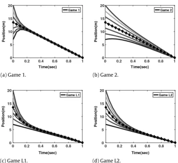
dependence on swarm population N is interesting. Only in Game L2, the convergence rate is independent of the population of the swarm, whereas in Game 1 it is proportional to the square root of N. In Games 2 and L1, the convergence rate of the agent’s trajectory depends on its position in the queue and increases as we go down to the last agent in the queue. The back-and-forth symmetry in the information structure implies that the center of the swarm follows a line. In the leader games, it plots a function of the same type as agent trajectories. As the information exchange among the swarm members gets sparser, the dependence of the trajectories on the initial conditions get lower. The consequence of this is that the initial positional configuration in a swarm is less preserved in looser information structures. Maximum swarm size values follow a similar pattern to this, in that, looser the information exchange, larger is the maximum swarm size.
Fig. 2verifies these conclusions on example trajectories that one observes in the resulting Nash equilibria in all four games of swarm with population N
=
7 and T=
1 under the same initial positions, attraction, and repulsion parameter values a=
40, r=
10. The trajectories of the swarm centers are shown marked with diamonds.5. Comments on generalizations of swarm games
Various assumptions that shape the motives of the agents in the games considered here are those that are needed to be able to obtain games with solutions as well as games that result in explicit analytic expressions for trajectories of the members of the swarm. Obviously, the most general information topology will be obtained if the parameters that weigh the attraction and repulsion terms as well as the target specification in the individual cost functions (the parameters a, r,
γ
, andβ
above in(1)and(2)) are allowed to be arbitrary positive numbers. Thus consider the game: Minimize for i=
1, . . . ,
N, Li:=
β
ixi(
T)
2+
T 0
ui(
t)
2 2+
N
j=1,j̸=i
aij[
xi(
t) −
xj(
t)]
2 2−
rij|
xi(
t) −
xj(
t)|
dt,
(8)subject to ui= ˙xifor i=1, . . . ,N, whereβ
i,aij, and rijare all positive. Our investigations indicate that in this more general formulation,
a Nash solution fails to exist. Mainly because the assumption of continuous strategies with respect to the initial positions prohibits any change of order. The assumptions on the relative size of the weights in the individual cost functions considered here are thus not arbitrary but necessary (since when they are violated, one can find suitable initial conditions for which a solution with the postulated order among the agents fails to exist). A collection of such counterexamples to existence of Nash equilibria is listed inYıldız and Özgüler(2016).
As an example, consider the order preserving property. It turns out to be closely tied to uniformity of attraction and repulsion parameters. It can actually be shown that, even if the attraction, repulsion, and foraging parameters are not equal but sorted like
aij
=
0 if i<
j,
aij.akj if i
≥
k,
rij
=
0 if i<
j,
rij
≫
rkj if i≥
k,
β
i≤
β
k if i≥
k,
where 0≪aNjand 0≪rj+1,j, then the ordering is again preserved. See Yıldız and Özgüler(2016) for a detailed proof. It is however difficult to quantify how close the adhesions or how far apart the repulsions need to be.
6. Conclusions
We have considered two non-cooperative swarming games of leader–follower information structures and identified appropriate assumptions under which unique Nash equilibria exist. The existence of a foraging task is irrelevant for aggregation stability and a swarm-like behavior still results. The accomplishment of the foraging task, when it is there, depends on whether the (foremost) leader has a desire to reach the target location at least as well as the other swarm members. We have also compared these two games with the earlier games (Özgüler & Yıldız, 2013;Yıldız & Özgüler, 2015) through analytic expressions and simulations. The generalization of these results to more than one dimension, especially to 3D, is obviously needed for potential robotics applications. Based on some preliminary simulation results on small population swarms, we are encouraged to continue our efforts in that direction.
References
Andersson, M., & Wallander, J. (2004). Kin selection and reciprocity in flight formation? Behavioral Ecology, 15(1), 158–162.
Basar, T., & Olsder, G. J.(1995). Dynamic noncooperative game theory, Vol. 200. SIAM.
Bressan, A., & Shen, W.(2004). Small BV solutions of hyperbolic noncooperative differential games. SIAM Journal on Control and Optimization, 43(1), 194–215.
Chatterjee, S., Goswami, D., Mukherjee, S., & Das, S.(2014). Behavioral analysis of the leader particle during stagnation in a particle swarm optimization algorithm. Information Sciences, 279, 18–36.
Chvátal, V.(1984). Perfectly ordered graphs. North-Holland Mathematics Studies, 88, 63–65.
Colbourn, C. J., Hoffman, D. G., & Rodger, C. A.(1991). Directed star decompositions of directed multigraphs. Discrete Mathematics, 97(1), 139–148.
Cutts, C., & Speakman, J.(1994). Energy savings in formation flight of pink-footed geese. Journal of Experimental Biology, 189(1), 251–261.
Estrada, E., & Vargas-Estrada, E.(2013). How peer pressure shapes consensus, leadership, and innovations in social groups. Scientific Reports, 3.
Gazi, V., & Passino, K. M.(2004). Stability analysis of social foraging swarms. IEEE Transactions on Systems, Man and Cybernetics, Part B: Cybernetics, 34(1), 539–557.
Hainsworth, F. R.(1988). Induced drag savings from ground effect and formation flight in brown pelicans. Journal of Experimental Biology, 135(1), 431–444.
Karimoddini, A., Lin, H., Chen, B. M., & Lee, T. H.(2013). Hybrid three-dimensional formation control for unmanned helicopters. Automatica, 49(2), 424–433.
Kawashima, H., & Egerstedt, M.(2014). Manipulability of leader–follower networks with the rigid-link approximation. Automatica, 50(3), 695–706.
King, A. J., & Cowlishaw, G.(2009). Leaders, followers, and group decision-making. Communicative & Integrative Biology, 2(2), 147–150.
Kirk, D. E.(2012). Optimal control theory: an introduction. Courier Corporation.
Lapierre, L., Soetanto, D., & Pascoal, A. (2003). Coordinated motion control of marine robots. In Proceedings of the 6th IFAC MCMC, Girona, Spain.
Nagy, M., Ákos, Z., Biro, D., & Vicsek, T.(2010). Hierarchical group dynamics in pigeon flocks. Nature, 464(7290), 890–893.
Özgüler, A. B., & Yıldız, A.(2013). Foraging swarms as Nash equilibria of dynamic games. IEEE Transactions on Cybernetics, 44(6), 979–987.
Peters, A. A., Middleton, R. H., & Mason, O.(2014). Leader tracking in homogeneous vehicle platoons with broadcast delays. Automatica, 50(1), 64–74.
Speakman, J. R., & Banks, D.(1998). The function of flight formations in greylag geese anser anser; energy saving or orientation? Ibis, 140(2), 280–287.
Wang, J., & Wang, D. (2008). Particle swarm optimization with a leader and followers. Progress in Natural Science, 18(11), 1437–1443.
Weimerskirch, H., Martin, J., Clerquin, Y., Alexandre, P., & Jiraskova, S.(2001). Energy saving in flight formation. Nature, 413(6857), 697–698.
Yıldız, A., & Özgüler, A.B. (2016). Foraging motion of swarms with leaders as Nash equilibria: Appendix.http://kilyos.ee.bilkent.edu.tr/~ayildiz/app.html. Yıldız, A., & Özgüler, A. B.(2015). Partially informed agents can form a swarm in a
Nash equilibrium. IEEE Transactions on Automatic Control, PP(99), 1–1.
Aykut Yıldız (S’10) received the B.S. and M.S. degrees in Electrical and Electronics Engineering Department from Bilkent University, Ankara, Turkey, in 2007 and 2010, respectively.
From July 2007 to August 2011, he was a research assistant in MİLDAR project funded by The Scientific and Technical Research Council of Turkey (TÜBİTAK). From September 2011 to now, he has been supported by the Servo Control Project by Military Electronics Industry Co. (ASELSAN). Currently, he is a Teaching and Research assistant and also a Ph.D. candidate at Electrical and
Electronics Engineering Department, Bilkent University, Ankara, Turkey. His current research interests are in Control Theory and Swarm Theory.
A. Bülent Özgüler received his Ph.D. at the Electri-cal Engineering Department of the University of Florida, Gainesville in 1982. He was a researcher at the Marmara Research Institute of TÜBİTAK during 1983–1986. He spent one year at the Institut für Dynamische Systeme, Bremen Universität, Germany, on Alexander von Humboldt Schol-arship during 1994–1995. He has been with the Electrical and Electronics Engineering Department of Bilkent Uni-versity, Ankara since 1986. He was at Bahçeşehir Univer-sity in 2008–2009 academic year, on leave from Bilkent University. Prof. Özgüler’s research interests are in the ar-eas of decentralized control, stability robustness, realization theory, linear matrix equations, and application of system theory to social sciences. He has about 60 re-search papers in the field and is the author of two books Linear Multichannel Con-trol: A System Matrix Approach, Prentice Hall, 1994 and, with K. Saadaoui, Fixed order controller design: A parametric approach, LAP Lambert Academic Publishing, 2010.