DESIGN OF A WIDEBAND AND
BI – DIRECTIONAL TRANSDUCER FOR
UNDERWATER COMMUNICATIONS
A THESIS
SUBMITTED TO THE DEPARTMENT OF ELECTRICAL AND ELECTRONICS ENGINEERING
AND THE INSTITUTE OF ENGINEERING AND SCIENCES OF BILKENT UNIVERSITY
IN PARTIAL FULLFILMENT OF THE REQUIREMENTS FOR THE DEGREE OF
MASTER OF SCIENCE
By
Işıl Ceren Elmaslı
April 2007
I certify that I have read this thesis and that in my opinion it is fully adequate, in scope and in quality, as a thesis for the degree of Master of Science.
Prof. Dr. Hayrettin Köymen (Supervisor)
I certify that I have read this thesis and that in my opinion it is fully adequate, in scope and in quality, as a thesis for the degree of Master of Science.
Prof. Dr. Ayhan Altıntaş
I certify that I have read this thesis and that in my opinion it is fully adequate, in scope and in quality, as a thesis for the degree of Master of Science.
Dr. Satılmış Topçu
Approved for the Institute of Engineering and Sciences:
Prof. Dr. Mehmet B. Baray
ABSTRACT
DESIGN OF A WIDEBAND AND BI – DIRECTIONAL
TRANSDUCER FOR UNDERWATER
COMMUNICATIONS
Işıl Ceren Elmaslı
M.S. in Electrical and Electronics Engineering
Supervisor: Prof. Dr. Hayrettin Köymen
April 2007
A two ceramic layer stacked transducer structure for short range underwater communications at high frequencies is studied in this work. The structure has a wide bandwidth of one octave and operates at 350 kHz center frequency. Transducer structure inherently has two electrical and two acoustic ports. Ceramic layers are matched to water load through quarter wavelength thick matching layers on each radiating face. Using electrical ports separately to compensate for the large acoustic length of the structure in water is also investigated. It is shown that the wide bandwidth operation can be maintained. The beamwidth of the structure is narrow due to end - fire effect of two back – to – back radiating elements.
ÖZET
SUALTI İLETİŞİMİ İÇİN GENİŞ BANDLI VE
ÇİFT – YÖNLÜ AKUSTİK ÇEVİRİCİ MODELLEMESİ
Işıl Ceren Elmaslı
Elektrik ve Elektronik Mühendisliği Bölümü Yüksek Lisans Tez Yöneticisi: Prof. Dr. Hayrettin Köymen
Nisan 2007
Bu tezde yüksek frekanslı kısa mesafe sualtı iletişimi için iki seramik katmanlı çevirici yapısı irdelendi. Yapının bir oktav genişliğinde çalışma bandı bulunmaktadır ve merkez çalışma frekansı 350 kHz’dir. Çevirici yapısında iki elektriksel, iki akustik port vardır. Seramik katmanlar her bir ışıma yapan yüzeyden su yüküne çeyrek dalga kalınlığındaki eşleştirici katmanlar aracılığıyla eşlenmişlerdir. Yapının sudaki uzun akustik boyunu dengelemek için elektriksel portların birer birer kullanılması incelenmiştir. Bu şekilde geniş bir bant aralığında çalışma sağlanmıştır. Yapının hüzme genişliği arka arkaya ışıyan elemanlardan dolayı dardır.
Anahtar Kelimeler: Akustik sualtı haberleşmesi, çevirici, geniş bant, geniş hüzme
Acknowledgements
I would like to express my gratitude to my supervisor Prof. Dr. Hayrettin Köymen for his instructive comments in the supervision
of the thesis.
I would like to express my special thanks and gratitude to the jury members Prof. Dr. Ayhan Altıntaş and Dr. Satılmış Topçu for evaluating my thesis.
I would also like to express my thanks to my parents and my husband Alper for their endless love and support throughout my life.
Contents
1. Introduction………..…...1 1.1 Historical References………..1 1.2 Communication Channel……….…2 1.3 Piezocomposite Materials………...3 1.4 Designing Transducer……….31.5 A Wideband and Bi – directional Transducer Design for Underwater Communications………5
1.6 Organization of the Thesis………..6
2. Analogy between Acoustics and Electromagnetics………..7
2.1 Wave Characteristics………..7
2.2 Power and Energy……….11
2.3 Boundary Conditions………11
2.3.1 Green’s function……….12
2.3.2 Rigid Baffle………14
2.3.3 Pressure Release Baffle………..15
3. Acoustic Underwater Transducer………17
3.1 Mason’s Model………..17
3.2 An Air-Backed Transducer in Air……….21
3.3 An Air - Backed Transducer in Water………..23
3.4 Transducer with Matching Layers………28
4. Wideband Bi – Directional Composite Piezoelectric Transducer…………....34
4.1 Properties……….…..34
4.2 Transmitting Mode………42
4.3 Receiving Mode………44
5. Reciprocal Operation…..………..47
5.1 Boundary Conditions……….47
5.2 Force Sensed at the Receiver Acoustic Ports………48
6.1 Changing the Distance within a Wavelength………57
6.2 Rotating the Receiving Transducer………...58
6.3 Fixed Frequency Response………61
6.3 Acoustic Face Dimensions………63
7. Conclusions………...……….65 8. Appendix I………..71 Green’s Function……….71 9. APPENDIX II...……….73 Transducer Matrix………...73 10. APPENDIX III………..………76 Derivation of F1 / Vs………76 11. APPENDIX IV…………..………81 Derivation of V1 / F1, when F2 = 0………..81 Derivation of V2 / F1 when F2 = 0………...84 12. APPENDIX V………...……….88
List of Figures
3. 1 Piezoelectric resonator of length ι with electrodes on opposite surfaces…… 17 3. 2 (a) Transducer, regarded as a three – port black box, (b) The force and
particle velocity notation on the transducer………18 3. 3 Mason series equivalent circuit………...20 3. 4 Electrical circuit of an air-backed and unloaded transducer in air…………..21 3. 5 Normalized admittance versus normalized frequency graph for an
air – backed and unloaded transducer in air………23 3. 6 Electrical circuit of an air-backed and transducer immersed in water………24 3. 7 Normalized admittance versus normalized frequency for air – backed
transducer immersed in water……….25 3. 8 Normalized conductance versus normalized frequency for an air – backed
transducer immersed in water with changing impedance of transducer…….26 3. 9 Normalized susceptance versus normalized frequency for an air – backed
transducer immersed in water with changing impedance of transducer…….26 3. 10 Normalized transfer function of an air – backed transducer immersed in
water; F2 / V3, where Z1 = Zwater , Z2 = 0 and 3 dB EffBW=12%...27 3. 11 Normalized transfer function of a transducer with backing material
immersed in water; F2 / V3 where Z1 = Z2 = Zwater, 3 dB EffBW=23%...28 3. 12 Transducer immersed in water with matching layers………29 3. 13 Normalized admittance versus normalized frequency of a transducer
matched to water Z1=Z2 = Zwater………..30
3. 14 Normalized admittance versus normalized frequency plots for a matched transducer with decreasing Zm…………..31
3. 15 Normalized admittance versus normalized frequency plots for a matched transducer with increasing Zm…………...32
3. 16 Normalized admittance versus normalize frequency plots for a matched transducer with decreasing. lm……….33
3. 17 Normalized admittance versus normalize frequency plots for a matched transducer with increasing. lm………..33
4. 1 Transducer structure made of 1 – 3 composite ceramic, matching and aluminium layers, where dark layers represents quarter – wavelength long matching layers, dotted layers are quarter – wavelength long piezoceramic
layers and the middle thin layer is the aluminium………..35
4. 2 Equivalent electrical model of proposed transducer structure………36
4. 3 Maximum flat admittance response of the proposed transducer………..39
4. 4 Maximum bandwidth admittance graph of the proposed transducer………...39
4. 5 Transfer function of maximum bandwidth transducer, F V when V1 1 2 is short circuited………...40
4. 6 Transfer function F2 / V1 when V2 is short circuited………41
4. 7 The circuit diagram of parallel connected transmitting transducer structure...42
4. 8 Transfer function F1 / Vs, where V1 = V2 = Vs…………...43
4. 9 Electrical model of receiving transducer model………...44
4. 10 Transfer function V1 / F1, when F2 is short circuited………..45
4. 11 Transfer function of V2 / F1 when F2 is short circuited………...46
5. 1 Proposed transducer structure radiates energy into two half – spaces……….47
5. 2 Acoustic waves radiating from the acoustic face………48
5. 3 Rotation of receiving transducer around its axes………50
5. 4 Transfer function V1 / Vs where F2 = 0………...52
5. 5 Transfer function V1 / Vs where F1 = 0……….…..52
5. 6 Transfer function V2 / Vs where F1 = 0……….……..53
5. 7 Transfer function V2 / Vs where F2 = 0……….…54
5. 8 Overall transfer function V1 / Vs………...55
5. 9 Overall transfer function V2 / Vs………...55
5. 10 Delayed and summed transfer function, 2 1 jw t s s V V e V V Δ + ……….…..56 6. 1 Transfer function 2 1 jw t s s V V e V V Δ + where distance between transducers are: (a) ZR = 10 m + λ / 4, b) ZR = 10 m + λ / 2, (c) ZR = 10 m + 3λ / 4,………...58
6. 3 Transfer functions where a) θ = 2o, b) θ = 5o, c) θ = 15o, d) θ = 22o, e) θ = 27o and f) θ = 90o. ... ….60 6. 4 Rotating the receiver around y - axis at fixed frequencies:... ..62 6. 5 Effective beamwidth versus normalized frequency. ... ..62 6. 6 Transfer functions 1 s F V , for A= 6 2 4 *10 m− and A =9 *10 m−6 2…... 63
6. 7 Polar plots for A= 4 *10 m−6 2 and A =9 *10 m−6 2when the receiving
transducer is rotated around its center (0≤θ≤2π), at a fixed frequency,
List of Tables
TABLE 1 ... 37 TABLE 2 ... 38
Chapter 1
Introduction
Underwater acoustic (UWA) communications is an interesting research field that shapes the abilities of people in shallow and deep waters. Preserving communication for long duration with a light weight and low battery power consumption becomes increasingly important for scuba divers, petrol inspectors and pollution analyzers [1]. Furthermore, the developments in piezoelectric materials make it possible to have more effective underwater communication applications.
1.1 Historical References
Leonardo Da Vinci is quoted to be the first one, who though it was possible to send and receive information in underwater. His discovery concerns the possibility of detecting a distant ship with a long tube submerged under the sea [2]. UWA communication systems are being used in underwater since 1905 [3]. A wire link between the diver and a surface communication point was used for voice communication [4]. Following the German submarine menace of 1st World War, researches are focused on the behavior of sound in underwater; besides its effects on submarine, surface ship, weaponry, and target locations [5]. SOund NAvigation
and Ranging term, “SONAR” was first used at that time. Echosounders are developed to detail bathymetry. Seismic and sidescan - sonar systems are evolved to map the sea floor and subsurface [6].
The U.S. Navy developed an underwater telephone to communicate with submarines by 1945 [2]. It was using a single - sideband suppressed carrier amplitude modulation in the range of 8 – 11 kHz. It was sending acoustic signals to several kilometers.
There has been a growing interest in the UWA communications in various application areas such as telemetry, remote control, and speech or image transmission in recent years. The bandwidth efficiency of proposed systems becomes an important issue in UWA communications [6].
1.2 Communication Channel
Acoustic propagation has physical constraints on the AUW channel, such as: Limited, range – dependent bandwidth, time varying multipath and low speed of sound (1500 m/sec) [7], [8]. The propagation range is low for high frequency channels. As a result, it is possible to send large bandwidth data over short distances.
On the other hand, the AUW systems includes barriers such as battery power, half – duplex communication and transducer bandwidth. The effective bandwidth of a transducer depends on the characteristics of materials used.
1.3 Piezocomposite Materials
The piezoelectric effect was discovered by Jacques and Pierre Curie in 1880. They found that when certain crystals are subjected to mechanical strain, they become electrically polarized and the degree of polarization is proportional to the applied strain [9]. The piezoelectric materials can convert mechanical energy into electrical and vice versa.
Piezoelectric ceramics are used in AUW transducer designs. The easy fabrication, lightweight and thickness properties, and thus high – sensitivity with better pressure stability characteristics are better than other transduction materials properties [10].
We prefer piezocomposite materials rather that piezoelectric ceramics because they offer increased sensitivity, broader bandwidth, improved impedance match to water and higher efficiency [11], [12]. Composite piezoelectric materials can be prepared by combining a piezoelectric ceramic with polymer layers [12], [13]. The geometry of these materials provides advantages such as high electromechanical coupling constant and acoustic impedance that can be matched to water through a matching layer. For the thesis, we prefer 30% PZT-5A and 70% stycast for the 1 – 3 composite ceramic layers.
1.4 Designing Transducer
Studies of Rayleigh, Pochammer, Chree, Lové, Bancroft and Davies developed the area of sound speed variability in rods [14]. The techniques based on implementation of piezoelectric transducer materials to transmission lines including transformer is introduced by Mason – the Mason Model, Redwood – the
Previous developments of transducer designs for underwater applications have shown that matching the structure to water with multiple matching layers is necessary for achieving a wide bandwidth, such as in the case of thin disk. The thin disk design highly depends on the properties of ceramic layers [16]. A common thin disk design is made by fixing two quarter – wavelength matching layers and connecting the structure to a half – wavelength PZT material. The thin disc structure is air – backed. It is immersed into water directed from a vibrating face. The thin disk design introduces narrow beamwidth reception characteristics which is advantageous in overcoming situations where multipath is a problem. The model is proper for using in upper band of 100 kHz to 1 MHz frequency region [17].
Another well – known transducer model is piston type. It is used for low frequency applications, 0 – 30 kHz. The model is constructed with metal – end pieces that act as resonators with central section of ceramic layer acting as the motor. Fabrication of the model is investigated by Neppiras [18] and Stansfield [19]. A broadband transducer is achieved by adding a quarter – wavelength matching layer to the loaded side of the structure. It has been shown that careful addition of other matching layers modifies the behavioral aspect of the transducer.
Many developers followed the former ones in developing piston – structure acoustic transducers. However, the problem with piston structures, mainly for low – frequency applications remained constant: Their voluminous and high weight due to structure being air backed limited the effective propagation areas and conditions of their application areas.
1.5 A Wideband and Bi – directional Transducer
Design for Underwater Communications
This work concerns design of a short range, wideband transducer. The band of the transducer is relatively wide when compared to other transduction elements.
Designing an omni – directional wideband transducer is not achievable for most of the transducer structures. The beamwidth of the transducer structure depends on the value of the radius to thickness ratio which is high compared to the wavelength of water. It also depends on the operational frequency.
The proposed transducer is achieved by connecting two quarter – wavelength composite piezoelectric layers with a thin aluminium layer. The piezocomposite layers are matched to water with quarter wavelength matching layers on both sides; besides they introduce two electrical ports to the transducer structure. We constructively add the electrical signals sensed at the electrical ports. The matching layers are beneficial for increasing the total throughput of energy when compared to an unmatched transducer structure. The aluminium layer is used for mounting, therefore the center of structure resists motion along any direction.
To sum up, the proposed structure can be explained as an acoustic transducer that uses another one for its backing property. The transducer structure provides capability of being used without any air – backing material that narrows the communication area to a half – space. The proposed structure provides full space communication. It is suitable for new communication techniques, such as spread spectrum applications, at short distances. When applied at high frequency range, it provides advantages like low power emission, and hence undetectability at a distance, as well as suitability for networking. The proposed design introduces new features for wideband transducer applications where the physical achievable
1.6 Organization of the Thesis
Chapter 2 introduces the analogy between acoustics and electromagnetics besides microwave theory. The general boundary conditions are discussed.
Chapter 3 summarizes several characteristics of transducers. We discuss the affects of backing materials; besides benefits of using quarter – wavelength matching layers.
Chapter 4 introduces the proposed wideband bi – directional transducer model. We discuss the transmitting and receiving modes of the proposed model.
Chapter 5 gives the propagation characteristics of a wave in underwater media. We discuss the propagation of a wave towards the half – space of the receiving transducer; the sensed acoustic forces on two acoustic ports of the receiver and the generated voltage at each electrical port.
Chapter 6 discusses the characteristics of the proposed transducer for several occasions based on the orientation of receiver and transmitter in underwater media.
The results of wideband bi – directional transducer structure on several studies are presented in Chapter 7. We also discuss future work that can be done to identify the potential of the proposed transducer structure.
Chapter 2
Analogy between Acoustics and
Electromagnetics
The wave properties of acoustics can be analyzed in a similar way with electromagnetic waves. This chapter details the analogy between acoustics and electromagnetics.
2.1 Wave Characteristics
Acoustics is the science of compressive waves in solids, liquids, or gases. There are two types of acoustic waves: (i) The longitudinal waves; the motion of a particle is in the same direction with the force applied to it. As a result, a force that is applied to the acoustic medium causes the medium to expand or contract in the same direction of it. (ii) The shear waves; the motion of the particle is transverse to the direction of force applied to it. Solids are subject to both shear and longitudinal waves; fluids do not support shear stress. Hence, throughout the thesis, we are concerned with only the longitudinal waves.
There are two fundamental differential equations for acoustic waves, based on conservation of mass and equation of motion.
Conservation of Mass: The relation between the particle velocity v and instantaneous density ρm is needed to be detailed in order to derive the relation of motion of the fluid with respect to its compression or expansion. For a volume of
element, the net rate at which mass flows into the volume through its surface must equal the rate at which the mass within its volume increases:
( ) 0 m mv t ρ ρ ∂ + ∇ ⋅ = ∂ . (2. 1)
We consider that ρm equals ρm0+ρm1, where ρm0 is the unperturbed density and ρm1 is the perturbation in the density. We assume that the direction of propagation and hence the displacement of material is in z direction. Assuming that v and ρm1 are first order perturbations, and keeping only first terms:
0 m 0 m v z t ρ ρ ∂ +∂ = ∂ ∂ , (2. 2) where ρm =ρm0 +ρm1=ρm0/(1+S)=ρm0(1−S). Thus, v S z t ∂ = ∂ ∂ ∂ . (2. 3)
S is the strain and proportional to stress T =cS, where c is the elastic constant of
the material.
Equation of Motion: The equation of motion of a point in a material, when a small time – variable stress is applied, can be solved using Newton’s second law. The net translational force per unit area applied to the material of length l is l T∂ /∂z, so the equation of motion is:
0 0 m m T v v z ρ ρ t ∂ = = ∂ ∂ ∂ . (2. 4)
Wave Equation: We combine the two acoustic differential equations Eq (2.3) and Eq. (2.4). They lead to:
2T ρ 2T
For a wave of radian frequency ω , with all field quantities varying as exp(j tω ), the solution to Eq. (2. 5) is in the form exp[ (j tω ±βaz)], where
1/ 2 0 ( m ) a s a c V ρ ω β =ω = , (2. 6)
is the propagation constant and 1/ 2 0 ( s ) a m c V ρ
= is the acoustic wave velocity. The
velocity of sound is approximately 1500 m/s in water, and ~1500 – 13000 m/s in solids. Hard materials such as metals and ceramics have greater velocities.
The phase velocity for an acoustic wave is: /
p a a
v =ω β = , V (2. 7)
and the group velocity is:
1/ 2 0
1/( / ) ( / )
g a s m a
v = dβ dω = c ρ =V , (2. 8)
which are same in a non-dispersive medium.
Acoustic Impedance: In analogy to Electromagnetic theory, we can define the acoustic impedance (specific acoustic impedance) Z as,
T Z
v
= − . (2. 9)
The characteristic electromagnetic impedance Z for air is ~377 ohms, while 0
the acoustic impedance for air at 200 is ~415 [Ns/m3-s] and for water at 200 is ~1.5 * 106 [Ns/m3-s].
Eq. (2.3) and Eq. (2.4) can be rewritten as follows:
v j T j S z c ω ω ∂ = = ∂ , (2. 10) and
0 m T j v z ωρ ∂ = ∂ . (2. 11)
These equations can be compared with the transmission line equations for voltage and current along a transmission line, which are;
V j LI z ω ∂ = − ∂ , (2. 12) and I j CV z ω ∂ = − ∂ , (2. 13)
where L is series inductance per unit length and C is the shunt capacitance per unit length. The propagation constant of a wave propagating along this line is
a LC
β =ω and its impedance isZ0 = L C/ .
Comparing the equations (2.3, 2.4, 2.12 and 2.13), it is seen that T is analogous to V and v is analogous to I. Therefore, stress and particle velocity solutions can be written as follows for a uniform plane wave confined to z – axis propagation. ( a ) ( a ) j t z j t z F B T T e= ω β− +T e ω β+ , (2. 14) and ( ) ( ) ˆ ( ) j t az j t az z F B v z =va =v e ω β− +v e ω β+ . (2. 15)
Eq (2.5) can be compared with the electromagnetic wave equation solution of a source free region:
2 2
0 0
(∇ +w μ ε )E= , 0 (2. 16)
which gets use of Maxwell’s equations:
0 , H E t E μ ∂ ∇ × = − ∂ ∂ (2. 17)
Comparing the Maxwell’s equations (Eq. 2.17) with Eq. (2.3 and 2.4), we conclude that velocity and stress, v and T are analogous to the electromagnetic field vectors, E and H . The significant difference between electromagnetic and acoustic waves is their attitude with respect to the propagating waves. E and H are both orthogonal to the direction of propagation, whereas v is generally a vector parallel to the direction of propagation and T is a scalar function of position. As a result, there is no polarization of acoustic waves, as there exists for electromagnetic waves.
2.2 Power and Energy
Acoustic power and energy definitions are similar to electromagnetic implementations. For a uniform plane wave in the time domain, acoustic power
density, or intensity is:
2 2
( ) ( ) ( ) / [ ]
s
I t = p t v t = p Z Wm−
. (2. 18)
The intensity of a uniform electromagnetic plane wave in the time domain is:
2 2
0
( ) ( ) ( ) / [ ].
I t =E t H t =E Z Wm− (2. 19)
2.3 Boundary Conditions
There are two acoustic boundary conditions to be satisfied for all times at all points on the boundary: (i) The acoustic pressures on both sides of the boundary must be equal and (ii) normal components of the particle velocities on both sides of the boundary must be equal.
For electromagnetic at every boundary: (i) The tangential component of electric field must be continuous across an interface and (ii) the normal component of magnetic field across an interface between two media must be continuous.
2.3.1 Green’s function
Green’s function is used to solve partial differentiation equations of electromagnetics and acoustics. The Green’s function is a technique to the solution of the partial differentiation equation that is obtained using a unit source (Impulse, Dirac Delta) as the driving function. The solution to the driving force is written as a superposition of the impulse response solutions (Green’s function) with the Dirac delta source at different locations, which in the limit reduces to an integral. The
Green’s function, jkR Ae G R −
= is a solution to the wave equation for a source point
at , ,x y z′ ′ ′ :
2G k G2 δ(x x y y z z′, ′, ′)
∇ + = − − − . (2. 20)
The derivation of Green’s function is as described in Appendix I.
Green’s theorem is useful to find a solution for the potential at a point due to excitation by a transducer. This is equivalent to finding the general solution forφat any point, given φ and ∇ on a surface surrounding the point , ,φ x y z . We multiply
the wave equation
2φ k2φ 0
∇ + = , (2. 21)
2G k G2 (x x y y z z, , )
φ∇ + φ =φδ − ′ − ′ − ′ . (2. 23)
After subtracting Eq. (2.22) from Eq. (2.23), we integrate the resulting expression over volume V, and obtain:
2 2 ( , , ) ( ) , ( , , ) ( ) . V V x y z G G dV x y z G G dV φ φ φ φ φ φ ′ ′ ′ ′ ′ = ∇ − ∇ ′ ′ ′ ′ = ∇ ∇ − ∇
∫
∫
i (2. 24)where the superscript indicates that the integration is done with respect to , ,x y z′ ′ ′
variables. Applying Gauss’s theorem to the integral reduces the equation to:
( , , ) ( ) s x y z G G φ φ φ ′ ′ ′ =
∫
∇ − ∇ i nds′, (2. 25)where s′ is any point enclosing the point , ,x y zand n is outward normal from the volume V. As a result, φ can be determined at any point if we know φand ∇ on φ the surrounding surface. This statement is also known as Helmholtz’s integral
theorem.
We assume that a piston transducer of area S1 is in a baffle of area S2 and the
rest of the enclosing surface volume is ∑ and RÆ∞ as z Æ ∞. When RÆ∞, both
φ and G Æ
jkR
e R
−
. This cancels out the two terms in the integral Eq. (2.23).
Sommerfeld Radiation condition makes the assumption of ignoring contributions to the integral from the surface at infinity. We can write the general Green’s function as 1 ( , , ) ( ) s x y z G G φ =
∫
φ∇ − ∇′ ′φ i nds′, (2. 26)where n is the normal pointing into the area of transducer and S1 is the area of
Eq. (2.24) can be simplified depending on the boundary conditions of φ and G and their derivatives onS1.
The most obvious way to simplify a solution for the equation is either to have
G=0 or ∂G z/∂ on the transducer and its baffle. Therefore, we only need to indicate / z∂ ∂ or φ φon the transducer. There are two specific boundaries that can be used based on the general Green’s function:
1) Rigid Baffle
2) Pressure Release Baffle
For both cases, we assume there exists a source (δ x x y y z z− ′, − ′, − ′)and its image (δ x x y y z z− ′, − ′, + ′) with respect to the plane z=0.
2.3.2 Rigid Baffle
The Green’s function can be written as following for a Rigid Baffle:
1 2 1 2 1 ( ) 4 jkR jkR e e G R R π − − = − + , (2. 27) where 2 2 2 1 2 2 2 2 ( ) ( ) ( ) , ( ) ( ) ( ) . R z z x x y y R z z x x y y ′ ′ ′ = − + − + − ′ ′ ′ = + + − + − (2. 28)
1 ( , , ) ( , ,0) 2 jkR z s e x y z u x y ds R φ π − ′ ′ ′ =
∫
, (2. 29)where u is the particle displacement along z – axis and z u= ∇ . φ
The Green’s function for Rigid baffle suits the boundary condition ∂G z′/∂ =0 at z′ =0. It specifies that there is no motion on the baffle and the normal component of the particle velocity is zero. If an acoustic wave impinges on the boundary, it completely reflects back. The given example is analogous to a dielectric boundary.
A rigid baffle is also analogous to an open circuited transmission line, such as the reflection coefficient on the baffle equals +1.
2.3.3 Pressure Release Baffle
For Pressure Release Baffle the Green’s function becomes:
1 2 1 2 1 ( ) 4 jkR jkR e e G R R π − − = − − . (2. 30)
This yields a solution for the potential at any point (z≥0) in the form
(1 1/ )cos ( , , ) ( , ,0) 2 jkR s jk e jkR x y z x y ds R θ φ φ π − + ′ ′ ′ =
∫
, (2. 31)where θ is the angle between the radius R and the z axis.
The Green’s function for Pressure Release baffle suits the boundary condition
G=0 at z′ =0. It specifies that the pressure on both sides of the boundary is equal. The given example is analogous to a conducting boundary.
A pressure release baffle is also analogous to a short circuited transmission line, such that the reflection coefficient on the baffle equals -1.
Chapter 3
Acoustic Underwater Transducer
Electromechanic transducers convert electrical energy into mechanical energy and vice versa. Therefore, they are used to transmit and receive media via acoustic waves in underwater.
3.1 Mason’s Model
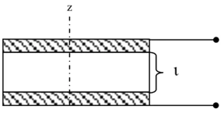
In Figure 3. 1, we consider a uniform transducer whose length,l is greater than its wavelength,λ and its electrodes on opposite surfaces are parallel to the z direction. We assume that Ex and Ey are zero, since the electrodes short out the
field.
Figure 3. 1. Piezoelectric resonator of length ι with electrodes on opposite surfaces.
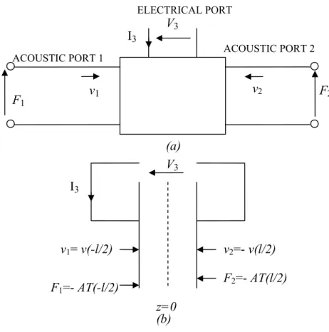
The piezoelectric transducer can be regarded as a three port black-box (Figure 3. 2) having two acoustic ports and an electrical port.
ι z
Figure 3. 2. (a) Transducer, regarded as a three – port black box, (b) The force and particle velocity notation on the transducer.
The force and particle velocity are similar to voltage and current for the electrical circuits. The external force that is applied to the piezocomposite material is
=
-F AT , (3. 1)
where A is the surface area of the transducer and T is the internal stress. The boundary conditions at the acoustic ports are:
1 2 1 2 = - ( / 2), = - ( / 2), ( / 2), ( / 2). F AT l F AT l v v l v v l − = − = − (3. 2) F1 v1 v2 ACOUSTIC PORT 1 V3 I3 ACOUSTIC PORT 2 F2 ELECTRICAL PORT I3 V3 F2=- AT(l/2) v2=- v(l/2) F1=- AT(-l/2) v1= v(-l/2) z=0 (a) (b)
We use Eq. (2.14) and Eq. (2.15) to derive the frequency domain equations for stress and velocity, where:
a a j z j z F B v v e= − β +v e β , (3. 3) and a a j z j z F B T T e= − β +T e β −hD. (3. 4) The following matrix is the general solution for a three port transducer:
1 1 2 2 3 3 0
cot
cos
cos
cot
1
C a C a C a C ah
Z
l
Z
ec l
w
F
v
h
F
j Z
ec l
Z
l
v
w
V
h
h
I
w
w
wC
β
β
β
β
⎡
⎤
⎢
⎥
⎢
⎥
⎡ ⎤
⎡ ⎤
⎢
⎥
⎢ ⎥
⎢ ⎥
= − ⎢
⎥
⎢ ⎥
⎢ ⎥
⎢
⎥
⎢ ⎥
⎢ ⎥
⎣ ⎦
⎢
⎥
⎣ ⎦
⎢
⎥
⎣
⎦
, (3. 5)where the clamped (zero strain) capacitance of the transducer is:
0 SA C l ε = . (3. 6)
Derivation of Mason’s Matrix is detailed in Appendix II.
We define the acoustic impedance of the piezocomposite material with surface area A, as:
0 c Z =Z A[kg/s], (3. 7) and 0 0 0 Z =ρ c [kg/m2-s], (3. 8)
where ρ0 is the density of piezocomposite material and c is the velocity of sound 0
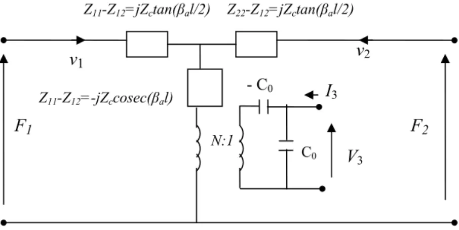
The Matrix given in Eq. (3.5) leads to the Mason circuit shown in Figure 3. 3. The right-hand and left-hand sides of the transducer circuit model are similar to each other with the exception of an extra potential hI3/ jw which is in series
with the potentials generated by v and 1 v . The circuit is analogous to a 2
transmission line if we assume that there is no net current through the electrical port. The transducer model employs a transformer, with transformer ratio:
0 0 s [ / ] eC eA N hC C m l ε = = = . (3. 9) The ratio 3 3 3 V Z
I = gives the input impedance of the transducer that can be find by
using the boundary conditions and the transducer matrix.
Figure 3. 3. Mason series equivalent circuit.
F1 F2 Z11-Z12=-jZccosec(βal) v1 - C0 C0 V3 N:1 v2 I3 Z11-Z12=jZctan(βal/2) Z22-Z12=jZctan(βal/2)
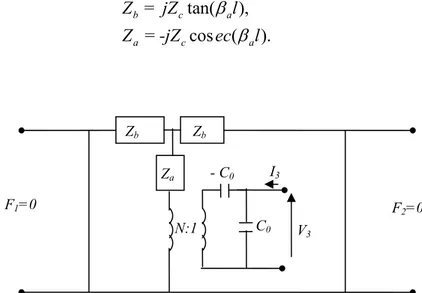
3.2 An Air-Backed Transducer in Air
We derive the properties of an air-backed and unloaded transducer in air. If we assume that acoustic port 1 provides the backing for the transducer and acoustic
port 2 is in air then the impedances of acoustic ports are Z1 = Z2 = 0 and
F1 = F2 = 0. The electrical equivalent circuit of the transducer is sketched in Figure 3. 4. where: = tan( ), = cos ( ). b c a a c a Z jZ l Z -jZ ec l β β (3. 10)
Figure 3. 4. Electrical circuit of an air-backed and unloaded transducer in air.
We use the Mason’s Matrix and derive the input impedance of the transducer as: 3 2 3 3 0 1 tan / 2 (1 ) / 2 a T a V l Z k I jwC l β β = = − , (3. 11)
where kT is the piezoelectric coupling constant for a transversely clamped material; for PZT-5A, kz2 is 0.33. Za N:1 C0 V3 Zb Zb - C0 I3 F1=0 F2=0
Eq. (3.11) shows that Z3 can be assumed as a capacitor C0 in series with motional impedance, Za: 2 0 tan / 2 / 2 T a a a k l Z jwC l β β = − . (3. 12)
The transducer introduces a parallel resonance with infinite electrical impedance. The transducer can be modeled as an inductance and capacitance in parallel at odd numbers of half – wavelengths long of transducer, where
(2 1)
al n
β = + π. The corresponding resonance frequency is given by the
relationship: (2 1) a n n V l π ω = + . (3. 13)
The transducer introduces zero electrical impedance at a frequency near ω0. The transducer behaves like a capacitance and inductance in series. The input impedance of the transducer is zero at frequency ω1, where:
2 tan / 2 1 / 2 a a T l l k β β = . (3. 14)
We consider the length of the transducer as half – wavelength long, and the resonance frequency of a half – wavelength transducer f0 is 400 kHz. The density
of the ceramic material is 2650 kg/m3 and velocity of sound, cc equals 4600 m/sec. The surface area, A of the square shaped layer is 9*10-6 m2. The radiation impedance of the ceramic Zc =A cρc c is 109.8 kg/s, whereρc cc = 12.2*106 kg/m2-s. The wavelength of ceramic layer,
0 c c
c f
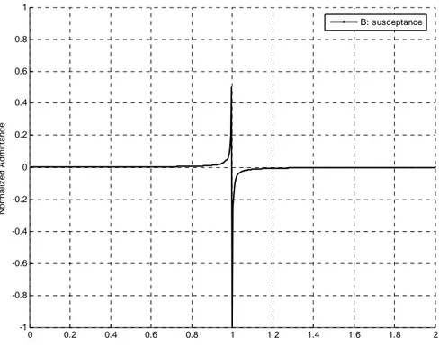
normalized admittance versus normalized frequency is sketched in Figure 3. 5. The susceptance seen at the input port is infinite at the resonance frequency.
0 0.2 0.4 0.6 0.8 1 1.2 1.4 1.6 1.8 2 -1 -0.8 -0.6 -0.4 -0.2 0 0.2 0.4 0.6 0.8 1 N or m al iz ed A dm it tanc e B: susceptance
Figure 3. 5. Normalized admittance versus normalized frequency graph for an air – backed and unloaded transducer in air.
3.3 An Air - Backed Transducer in Water
The air - backed half – wavelength long transducer is placed with its front surface in water. The impedance of water acts as load introduced to the front acoustical surface of the transducer, where Z1 = 0 and Z2 = Zw. The radiation
impedance of water is 13.5 kg/s, the density of waterρwequals 1000 kg/m3, velocity of sound c is 1500 m / sec and A = 9*10w -6 m2. The acoustic impedance of transducer is greater compared to the acoustic impedance of water.
Figure 3. 6. Electrical circuit of an air-backed and transducer immersed in water.
We derive the input impedance of the air - backed half – wavelength long transducer immersed in water at its resonance frequency using the matrix given in Eq. (3.5), where: 2 3 0 0 4 T c w k Z Z C Z πω = . (3. 15)
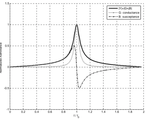
The normalized admittance versus normalized frequency is as sketched in
Figure 3. 7. Its susceptance is zero at the resonance frequency of a half – wavelength long transducer. The real part of the function is symmetric
around its resonance frequency. Za N:1 C0 V3 Zb Zb F1=0 -C0 F2 Zw I3
0 0.2 0.4 0.6 0.8 1 1.2 1.4 1.6 1.8 2 -1 -0.5 0 0.5 1 1.5 N or m al iz ed A dm it tanc e f / f 0 |Y|=|G+jB| G: conductance B: susceptance
Figure 3. 7. Normalized admittance versus normalized frequency for air – backed transducer immersed in water.
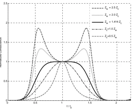
If the transducer structure is replaced with another one that has lower acoustic impedance, then the input impedance (Eq. 3.15) decreases and the 3 dB effective bandwidth of the transducer to increase. We demonstrate the change of the admittance response of transducer with respect to changes in acoustic impedance of transducer when the transducer structure is immersed in water, in Figure 3. 8 and Figure 3. 9. The bandwidth of the conductance increases when the impedance of transducer becomes close to the impedance of water (Figure 3. 8). For
1/ 2
w c
Z = Z the admittance response of transducer is flat. When
w
Z >1/ 2Zcthere are peaks on both sides of f0. There is a sharp response near f=f0
as the acoustic impedance of transducer is increased. When Zw/Z is very large the c
peaks tend to occur at f=0.5f0 and f=1.5f0. The susceptance at the resonance
frequency is not affected from changing the characteristic impedance; it is zero for all values (Figure 3. 9).
0 0.5 1 1.5 2 0 0.5 1 1.5 2 2.5 N or m al iz e d C ond uc tan c e f / f0 Zw = 2.5 Zc Zw = 2.0 Zc Zw = 1.414 Zc Zc=1.0 Zw Z c=0.5 Zw
Figure 3. 8. Normalized conductance versus normalized frequency for an air – backed transducer immersed in water with changing impedance of transducer.
0 0.2 0.4 0.6 0.8 1 1.2 1.4 1.6 1.8 2 -1.5 -1 -0.5 0 0.5 1 1.5 N or m al iz e d S us c ept an c e f / f0 Zw = 2.5 Zc Zw = 2.0 Zc Zw = 1.414 Zc Zc=1.0 Zw Zc=0.5 Zw
Figure 3. 9. Normalized susceptance versus normalized frequency for an air – backed transducer immersed in water with changing impedance of transducer.
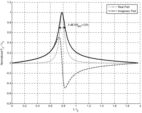
We feed the transducer with unit impulse via its electrical port, V3
(Figure 3. 6). The transfer function F2 / V3 of the radiating acoustic port is
examined. F2 is the force generated at the receiving acoustic port and V3 is the
voltage at the transmitting electrical port. The transfer function is as depicted in Figure 3. 10. The 3 dB effective bandwidth of the function is 12%. Its effective resonance frequency is less than the resonance frequency of a half – wavelength ceramic layer. This is due to the effect of negative capacitance, -C0.
0 0.2 0.4 0.6 0.8 1 1.2 1.4 1.6 1.8 2 -0.8 -0.6 -0.4 -0.2 0 0.2 0.4 0.6 0.8 1 1.2 N or m al iz ed F 2 / V 3 f / f 0 Real Part Imaginary Part 3 dB Eff BW=12%
Figure 3. 10. Normalized transfer function of an air – backed transducer immersed in water; F2 / V3, where Z1 = Zwater , Z2 = 0 and 3 dB EffBW=12%.
Instead of using an air-backing material at the acoustic port 1 (Figure 3. 6), we adjust a quarter – wavelength layer whose impedance equals to the radiation impedance of water, Z1 = 13.5kg s . When a unit impulse is radiated from the /
electrical port of the transducer, the transfer function of force generated on an acoustic port F2, F2 / V3, becomes as depicted in Figure 3. 11. The magnitude of the
(Figure 3. 10). However, its 3 dB effective bandwidth is greater than the air – backed transducer, it is 23 %.
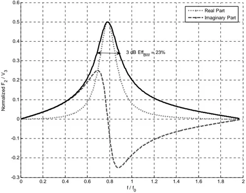
0 0.2 0.4 0.6 0.8 1 1.2 1.4 1.6 1.8 2 -0.3 -0.2 -0.1 0 0.1 0.2 0.3 0.4 0.5 0.6 N or m al iz ed F 2 / V 3 f / f 0 Real Part Imaginary Part 3 dB Eff BW = 23%
Figure 3. 11. Normalized transfer function of a transducer with backing material immersed in water; F2 / V3 where Z1 = Z2 = Zwater, 3 dB EffBW=23%.
3.4 Transducer with Matching Layers
We assume that both sides of the transducer are terminated with quarter wavelength matching layers. The transducer is immersed in water, Z1=Z2 = Zwater.
Figure 3. 12. Transducer immersed in water with matching layers.
We demonstrate the impedance values of matching layers with Zam and Zbm
abbreviations, where: Z = jZ tan( 2 ), Z = -jZ cosec ( ), m m bm m am m m m l l β β (3. 16) and Z , , 2 . m m m m m m m A c C f ρ λ π β λ = = = (3. 17)
the radiation impedance of matching layer is Zm = 27kg s . / ρm equals 3000
kg/m3 and c equals 1000 m/s. The wavelength of the matching layer, m λm is
0.0025 m at the resonance frequency of a half – wavelength ceramic,
f0 = 400 kHz. Its length,
4
m m
l =λ is 0.625 mm. The propagation constant βm equals 2.51*103.
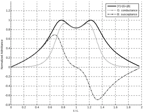
The admittance realized right after the transformer is shown in Figure 3. 13. The function employs two symmetric peaks. The transducer is much more
F2 Zbm Zbm Zb Zb Zbm Za - C0 C0 F1 V3 N:1 Zam Z1 Zam Z2 Zbm
effective compared to the transducer immersed in water with no matching layers. The matching layers improve the bandwidth of admittance function.
0 0.2 0.4 0.6 0.8 1 1.2 1.4 1.6 1.8 2 -0.8 -0.6 -0.4 -0.2 0 0.2 0.4 0.6 0.8 1 1.2 N or m al iz ed A dm it tanc e f / f 0 |Y|=|G+jB| G: conductance B: susceptance
Figure 3. 13. Normalized admittance versus normalized frequency of a transducer matched to water
Z1=Z2 = Zwater.
We demonstrate the effect of decreasing the acoustic impedance of matching layers, Zm in Figure 3. 14. The impedance graphs are sketched for 100%, 95%,
90%, 83%, 75% and 65% values of Zm. The normalized admittance value seen
from the electrical ports at the resonance frequency, f0 increases as Zm decreases.
On the other hand, the effective frequency band remains unchanged as the acoustic impedance of matching layer decreases. The admittance has only one peak at the resonance frequency f0, when the matching layer acoustic impedance values are
greater than 83%. For 83% Zm,the admittance response of transducer is flat. There
are two peaks on both sides of f0 for acoustic impedance of matching layers greater
0 0.2 0.4 0.6 0.8 1 1.2 1.4 1.6 1.8 2 0 0.2 0.4 0.6 0.8 1 1.2 1.4 1.6 1.8 2 N or m al iz ed A dm it tanc e f / f 0 100% Z m 95% Z m 90% Z m 83% Z m 75% Z m 65% Z m
Figure 3. 14. Normalized admittance versus normalized frequency plots for a matched transducer with decreasing Zm.
We demonstrate the effect of increasing the impedance of matching layers, Zm
in Figure 3. 15. The impedance graphs are sketched for 100%, 105%, 110%, 115%, 120% and 145% values of Zm. The normalized admittance value seen from
the electrical ports at the resonance frequency, f0, decreases as the percentage of Zm
increases. The peaks tend to move away from the resonance frequency as Zm
0 0.2 0.4 0.6 0.8 1 1.2 1.4 1.6 1.8 2 0 0.2 0.4 0.6 0.8 1 1.2 1.4 N or m al iz ed A dm it tanc e f / f 0 100% Z m 105% Z m 110% Z m 115% Z m 120% Z m 145% Z m
Figure 3. 15. Normalized admittance versus normalized frequency plots for a matched transducer with increasing Zm.
We demonstrate the effect of decreasing the length of matching layers, lm in
Figure 3. 16. The impedance graphs are sketched for 100%, 95%, 90%, 85%, 80% and 65% values of lm where lm =625 μm. When the length of admittance layer is
less than 80% lm, the admittance has only one peak, which occurs below the
resonance frequency f0. The peak moves towards the resonance frequency, f0, as the
length of matching layer is decreased further. The admittance at the resonance frequency, f0 increases as the length of matching layer decreases.
We demonstrate the effect of increasing the length of matching layers, lm in
Figure 3. 17. The impedance graphs are sketched for 100%, 105%, 110%, 115%, 120% and 130% values of lm. The admittance tends to have only one peak as the
0 0.2 0.4 0.6 0.8 1 1.2 1.4 1.6 1.8 2 0 0.2 0.4 0.6 0.8 1 1.2 1.4 1.6 1.8 N o rm a liz ed A d m it tanc e f / f0 100% lm 95% lm 90% lm 85% lm 80% lm 65% lm
Figure 3. 16. Normalized admittance versus normalize frequency plots for a matched transducer with decreasing. lm. 0 0.2 0.4 0.6 0.8 1 1.2 1.4 1.6 1.8 2 0 0.2 0.4 0.6 0.8 1 1.2 1.4 1.6 1.8 2 N o rm a liz ed A d m it tanc e f / f0 100% lm 105% lm 110% lm 115% lm 120% lm 130% lm
Figure 3. 17. Normalized admittance versus normalize frequency plots for a matched transducer with increasing. lm.
Chapter 4
Wideband Bi – Directional Composite
Piezoelectric Transducer
The proposed transducer structure has a wide bandwidth; besides it can be used to receive and send acoustic waves to the two half – spaces orthogonal to its radiating faces. This chapter details the characteristics of receiving and transmitting modes of the transducer.
4.1 Properties
The proposed transducer structure is composed of matching, aluminium and 1 - 3 composite ceramic layers as shown in Figure 4. 1. The layers are square shaped; having surface area, A = 9*10-6 m2. The two radiating faces (to each half space) of the transducer are displaced by the length of the structure. The displacement is about 2 wavelengths in water at resonance frequency, with available materials. The proposed transducer employs two electrical ports, V1 and
V2; besides two acoustic ports, F1 and F2 as depicted in Figure 4. 2.
The transducer structure has two back-to-back quarter wavelength thick 1 - 3 composite piezoelectric elements at its resonance frequency. Each element
provides the rigid, or high impedance backing to the other element, maintaining efficiency. The structure has advantages compared to a half - wavelength
transduction element, such as; the acoustic forces received on two acoustic ports can be used to derive constructive linear combinations of two signals.
The ceramic layers are separated by a thin aluminium layer as shown in Figure 4. 1. The aluminium layer is not required from the performance point of view but it is included to provide a mounting support. Thus, the interface between two ceramic elements is a stress node.
We use quarter wavelength matching layers to match each piezocomposite layer to water. Acoustic matching provides the expected wide bandwidth to each element.
Figure 4. 1. Transducer structure made of 1 – 3 composite ceramic, matching and aluminium layers, where dark layers represents quarter – wavelength long matching layers, dotted layers are
quarter – wavelength long composite piezoelectric layers and the middle thin layer is the aluminium.
The equivalent electrical model of the transducer is shown in Figure 4. 2. Ceramic layers are modeled using Mason’s circuit model. The Mason’s equivalent model of 1 - 3 composite ceramic layer includes the transformer ratio ‘N’ as stated in Eq (3.9) where,
z
y
2 2 0.017[ / ] [ / ], 5.3 / . eA N kg m s C m l e C m = ≈ = = (4. 1)
We sketch the aluminium and matching layers with their transmission line equivalent models.
Figure 4. 2. Equivalent electrical model of proposed transducer structure.
We use 30% PZT-5A and 70% stycast for the 1 – 3 piezocomposite layers [13]. The layers are each λ/ 4=2.875 mm long, where λ=c f0and f is the 0
resonance frequency of a half - wavelength transducer, 400 kHz. The characteristic impedance of each composite piezoelectric layer is 12.2*106kg m s . The wave / 2
velocity in the composite material c equals 4600 m/sec. Table I gives detailed data describing the properties of composite PZT-5A and stycast. Using the properties of piezocomposite layer, the clamped capacitance, C0 is calculated to be7.2 pF.
The aluminium layer is 1 mm thick. The layer has characteristic impedance of 16.2 *106kg m s . The wave velocity of the aluminium layer is 6000 m / sec and / 2
its density is 2700 kg / m3.
- C0
C0
- C0
ιm ι ιal ι ιm
Ceramic layer 1 Ceramic layer 2
Matching layer 1 Aluminium layer Matching layer 2
N:1 C0 Zam Zbm Zbm Zbm Zam Zb Zb Za Zbl Zbl Zb Zb Zbm Zal Za F1 F 2 V1 N:1 V2
The transducer structure is about 8 mm long at the resonance frequency of a half – wavelength transducer, f0.
Table II presents detailed information about the transducer layers. The values reflect their figures at 400 kHz.
TABLE 1
COMPOSITE PZT-5A and STYCAST PROPERTIES
PZT-5A Stycast
Relative dielectric constant,
free 1700
T
ε ε330 =
Relative dielectric constant,
clamped 850 S ε ε330 = Elastic Stiffness c D 14.7 *1010N m/ 2 33 = 10 2 11.1*10 / S c33 = N m 9 2 7.66 *10 / S c = N m Frequency Constant of a thin plate 3t 1890( . ) N = Hz m
Acoustic wave velocity 4350
l V = m/sec Vl =2750m/sec density ρ=7750kg m/ 3 ρ =1160kg m/ 3 Piezoelectric constant 2 33 15.8 / e = C m Characteristic Impedance 6 2 33.7*10 / c Z = kg m − s 3*106 / 2 s Z = kg m −s
TABLE 2
TRANSDUCER COMPONENTS
Matching layer Piezocomposite layer Aluminium layer
Surface Area 6 2 9 *10 A= − m 6 2 9 *10 A= − m 6 2 9 *10 A= − m Length 625 m l ≈ μm l=2.875mm lal =1.0mm Wavelength 2.5 m mm λ = λ=11.5mm λal =15.0mm Propagation constant 3 2.51*10 m β = β =546.4 *103 3 418.9 *10 al β = Density 3000 / 3 m kg m ρ = ρ=4600kg m/ 3 2700 / 3 al kg m ρ = Bulk velocity of sound cm=1000 /m s c=2652 /m s cal =6000 /m s Acoustic Impedance Zm =ρm mc A 27kg/ s = 109.8 / s Z cA kg ρ = = 145.8 / s alu al al Z c A kg ρ = = am m m m
Z = - jZ cosec (β l ) Z = - jZcosec ( l)a β Z = - jZ cosec (al alu βal all )
bm m m m
Z = jZ tan (β l / 2) Z = jZtan ( l / 2)b β Z = jZ tan (bl alu βal all / 2)
The effective bandwidth of the transducer can be changed by using different length and impedance of matching layers for fine tuning. In order to achieve a wideband transducer, we analyze the admittance seen from the acoustic ports. In Figure 4. 3 and Figure 4. 4, the normalized admittance versus normalized frequency graphs are sketched for the maximum flat admittance and the maximal bandwidth admittance. The matching layer properties of the maximum flat admittance graph are taken as lm≈0.308λm and Z = 21.9m kg s . The matching / layer properties of the maximum bandwidth admittance graph are lm≈0.278λmand
m
Z = 30 kg s . We derive the maximum bandwidth response according to the two / way transfer function of a transducer. We allow the variation of the two way transfer function of a reciprocal operation down to 70% of its maximum value. As a result, the ripples within Figure 4. 4 are accepted. Detailed examination of reciprocal operation can be found inChapter 5.
0 0.2 0.4 0.6 0.8 1 1.2 1.45 -0.6 -0.4 -0.2 0 0.2 0.4 0.6 0.8 1 1.2 f / f0 N o rm a li z ed A d m it tan c e Real Part Imaginary Part
Figure 4. 3. Maximum flat admittance response of the proposed transducer.
0 0.2 0.4 0.6 0.8 1 1.2 1.45 -0.4 -0.2 0 0.2 0.4 0.6 0.8 1 f / f0 N o rm a li z ed A d m it tan c e Real Part Imaginary Part
The resonance frequency of the maximum flat response (Figure 4. 3) is less than that of the maximum bandwidth response. Both values are comparably less than the resonance frequency of a half wavelength transducer, f , as expected. 0
We excite the maximum bandwidth response transducer while the electrical port 2 is short circuited. The transfer function F V of the radiating port F1 1 1, due to
the unit impulse,V is as depicted in Figure 4. 5. The real part of function decays 1
fast above the frequencies, f ≈1.4f0. The imaginary part of the transfer function is negative for f ≥0.6f0. 0 0.2 0.4 0.6 0.8 1 1.2 1.4 1.6 -0.015 -0.01 -0.005 0 0.005 0.01 0.015 0.02 F1 / V1 , V 2 = 0 f / f0 Real Part Imaginary Part
Figure 4. 5. Transfer function of maximum bandwidth transducer, F V1 1 when V2 is short
circuited.
The transfer function F V of the radiating port F2 1 2, due to the unit impulse
above frequencies, f ≈1.4f0. The imaginary part of the transfer function is negative between0.55f0 ≤ ≤f 1.05f0. 0 0.2 0.4 0.6 0.8 1 1.2 1.4 1.6 -0.01 -0.005 0 0.005 0.01 0.015 0.02 F2 / V1 , V 2 = 0 f / f0 Real Part Imaginary Part
Figure 4. 6. Transfer function F2 / V1 when V2 is short circuited.
We consider exciting the transducer with an impulse, when the electrical port V1 is short circuited. Using the reciprocity theorem the transfer function
1 2
F V , of force generated on the acoustic port F1, due to the impulse applied to V 2
is similar to the transfer function shown in Figure 4. 6. The transfer function
2 2
F V , of force generated on the acoustic port F2, due to the impulse applied to V 2
is similar to the transfer function shown in Figure 4. 5.
2 1 1 2 1 2 1 0 2 0 1 2 2 0 1 0 , . V V V V F F V V F F V V = = = = = = (4. 2)
4.2 Transmitting Mode
The proposed transducer structure is enhanced to be used for both transmit and receive modes in underwater. The transducer circuit in transmitting mode is shown in Figure 4. 7. Electrical ports V1 and V2 are fed by the voltage source, Vs, to
maintain a parallel connection. The details of circuit parameters are given in Table II.
Figure 4. 7. The circuit diagram of parallel connected transmitting transducer structure.
We immerse the transducer structure in water, so that Z1 = Z2 = Zwater
(Figure 4. 7). We excite the electrical ports of transducer with unit impulse by applying voltage through Vs. This causes acoustic forces to be generated on the
acoustic ports F1 and F2. Due to the symmetry of the transducer structure, equal
magnitudes of forces are generated at two radiating acoustic faces (F1 = F2).
The proposed transducer structure doesn’t include any tuning devices for the electrical ports V1 and V2, since they decrease the total output power.
Zbm Zam Za Zbl Zal Zb Zb Za Zbm Zam - C0 C0 - C0 V1 V2 N:1 N:1 Vs Vg F1 F2 Zbm Z2 Zbm Zb Zb Zbl Z1 C0
Figure 4. 8 shows the transfer function F1 / Vs of total force generated on the
acoustic port F1 due to the impulse excited on parallel connected electrical ports V1
and V2,, versus normalized frequency. The 3 dB bandwidth of the transfer function
is 87 %. Its resonance frequency is 0.856f0.
The summation of transfer functions
2 1 1 V 0 F V = (Figure 4. 5) and 1 1 2 V 0 F
V = (Figure 4. 6) equals the transfer function
1 s
F
V (Figure 4. 8). The resonance
function is not symmetric around f0, since the negative capacitance C0 causes a decrease in center frequency. The transfer function F2 / Vs is identical to the
transfer function F1 / Vs, since V1 = V2 = Vs.
The derivation of the response function F1 / Vs is detailed in Appendix III.
0 0.2 0.4 0.6 0.8 1 1.2 1.4 1.6 -8 -6 -4 -2 0 2 4 6 8 10x 10 -3 F1 / V s f / f 0 Real Part Imaginary Part 3 dB Eff BW = 87%
4.3 Receiving Mode
The equivalent electrical circuit of the proposed transducer structure in receiving mode is sketched in Figure 4. 9. We connect feedback amplifiers to the electrical ports. They cancel the effect of positive capacitance due to virtual
ground. The positive port of feedback amplifier is grounded. Its negative port is connected to the negative capacitance, - C0. Zload is inserted between the negative
port and voltage outputs, V1 and V2. Zload equals the equivalent real impedance seen
before the transformer.
Acoustical wavesare sensed by the acoustic ports (F1 and F2) in receive mode.
The signals are converted to electrical pulses by the transformer.
Figure 4. 9. Electrical model of receiving transducer model.
The transfer function V1 / F1, of voltage generated on the electrical port V1 with
respect to the unit force generated at acoustic port F1, when F2 is short circuited is
as shown in Figure 4. 10. The 3 dB effective bandwidth of V1 / F1 equals 73.7%. The 3 dB bandwidth of the receiving mode transfer function is less than the 3 dB bandwidth of transmitting mode function. The function has two peaks, its real part is positive above f≈1.05 f0. Its imaginary part passes through zero at f≈0.6 f0. The magnitude of the receiving mode transfer function is greater than the magnitude of the transmitting mode transfer function (Figure 4. 8), due to the transformer ratio on the order of 0.016. Zbm Zbm Zb Zb Za Zam Z1 Zbl Zbl Zal Zb Zb Za Zbm Z2 - C0 C0 F2 V1 Vg -+ Zload - C0 C0 -+ Zbm Zbm N:1 N:1 Zload V2 F1
0 0.2 0.4 0.6 0.8 1 1.2 1.4 1.6 -60 -40 -20 0 20 40 60 80 f / f 0 V1 / F1 , F2 = 0 Real Part Imaginary Part 3 dB Eff BW = 73.7%
Figure 4. 10. Transfer function V1 / F1, when F2 is short circuited.
The transfer function V2 / F1 of voltage generated on the electrical port V2 with
respect to a unit force generated at acoustic port F1, when F2is short circuited is as
shown in Figure 4. 11. The 3 dB effective bandwidth of V2 / F1 is 71%. The derivation of transfer functions
2 1 1 F 0 V F = and 2 2 1 F 0 V F = are given in Appendix IV.
0 0.2 0.4 0.6 0.8 1 1.2 1.4 1.6 -60 -40 -20 0 20 40 60 80 f / f 0 V2 / F1 , F2 = 0 Real Part Imaginary Part 3 dB Eff BW = 71%
Chapter 5
Reciprocal Operation
This chapter details the reciprocal operation of the proposed transducer structure. Reciprocal operation is considered as propagation of acoustic wave from a transducer and reception at the acoustic port of another transducer, where the transducers are separated by a distance.
5.1 Boundary Conditions
The proposed transducer structure radiates equal acoustic waves into two half – spaces through its radiating ports (Figure 5. 1). The proposed transducer structure is assumed to be mounted on an infinite baffle.
Figure 5. 1. Proposed transducer structure radiates energy into two half – spaces.
The right acoustic face is separated by a distance z0 from the center of the
transducer and radiates acoustic waves towards +z direction. The left acoustic face is separated a distance z0 from the center of the transducer but radiates towards –z
direction. Their magnitudes are the same. The radiating power from the acoustic faces result in finite potential at z = 0 plane. However, there is no net
x
displacement. The tangential components of the wave velocities are canceled by each other.
This assumption is consistent with the Rigid Baffle boundary definition, where there is no net displacement outside the baffle. However, there is a significant difference between the Rigid Boundary definition stated in Chapter 2 and the boundary condition of the proposed transducer structure. The former one radiates energy into one – half space and uses the image theory for basis; the latter one radiates energy into two – half spaces, and the waves propagated to the z=0 plane have 180 degrees phase difference.
5.2 Force Sensed at the Receiver Acoustic Ports
Based on the above assumption, we consider that the acoustic faces radiate energy towards the half – space that they their normal’s direct as shown in Figure 5. 2. x y R1 R2 R TX RX Z = ZR
Figure 5. 2. Acoustic waves radiating from the acoustic face.
R: Distance between the radiating acoustic port and the center of the receiving port; R1: Distance
between the radiating acoustic port and the front receiving port; R2: Distance between the radiating